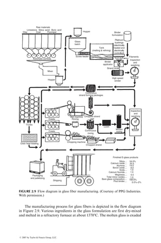
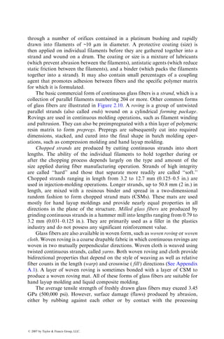
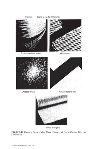
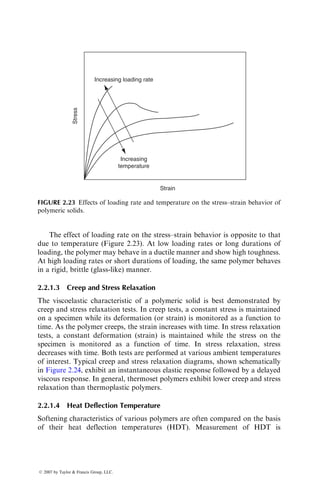
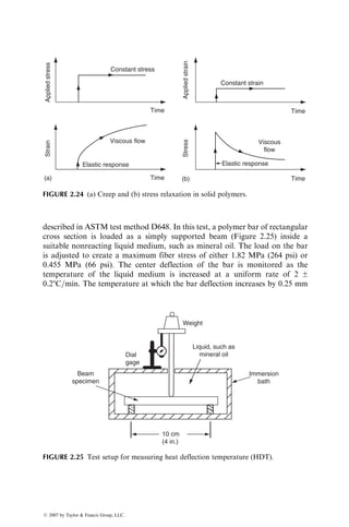
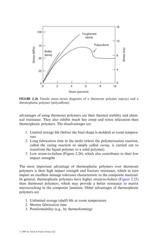
This document provides an overview of the third edition of the textbook "Fiber-Reinforced Composites: Materials, Manufacturing, and Design" by P.K. Mallick. The textbook covers topics such as fiber and matrix materials, mechanics of composites, performance of composites, manufacturing processes, design considerations, and special types of composites including metal matrix, ceramic matrix, and polymer nanocomposites. The textbook contains chapters on these topics along with examples, problems, and appendixes providing additional information.


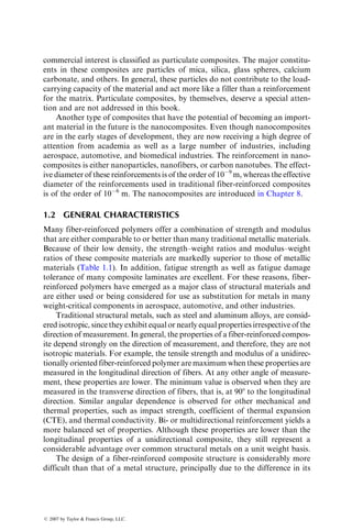
![The composite applications on commercial aircrafts began with a few
selective secondary structural components, all of which were made of a high-
strength carbon fiber-reinforced epoxy (Table 1.4). They were designed and
produced under the NASA Aircraft Energy Efficiency (ACEE) program and
were installed in various airplanes during 1972–1986 [1]. By 1987, 350 compos-
ite components were placed in service in various commercial aircrafts, and over
the next few years, they accumulated millions of flight hours. Periodic inspec-
tion and evaluation of these components showed some damages caused by
ground handling accidents, foreign object impacts, and lightning strikes.
TABLE 1.3
Early Applications of Fiber-Reinforced Polymers in Military Aircrafts
Aircraft Component Material
Overall Weight
Saving Over
Metal Component (%)
F-14 (1969) Skin on the horizontal stabilizer
box
Boron fiber–epoxy 19
F-11 Under the wing fairings Carbon fiber–epoxy
F-15 (1975) Fin, rudder, and stabilizer skins Boron fiber–epoxy 25
F-16 (1977) Skins on vertical fin box, fin
leading edge
Carbon fiber–epoxy 23
F=A-18 (1978) Wing skins, horizontal and
vertical tail boxes; wing and
tail control surfaces, etc.
Carbon fiber–epoxy 35
AV-8B (1982) Wing skins and substructures;
forward fuselage; horizontal
stabilizer; flaps; ailerons
Carbon fiber–epoxy 25
Source: Adapted from Riggs, J.P., Mater. Soc., 8, 351, 1984.
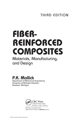
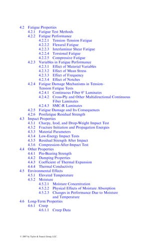
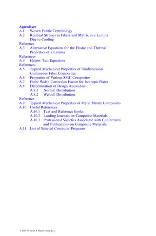
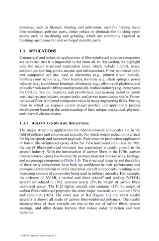
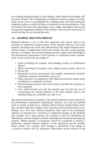
FIGURE 1.1 Stealth aircraft (note that the carbon fibers in the construction of the
aircraft contributes to its stealth characteristics).
ß 2007 by Taylor Francis Group, LLC.](https://image.slidesharecdn.com/fiberreinforcedcompositesmaterialsmanufacturinganddesignp1-220510152925-9ef3de0d/85/Fiber_Reinforced_Composites_Materials_Manufacturing_and_Design_P-1-pdf-25-320.jpg)
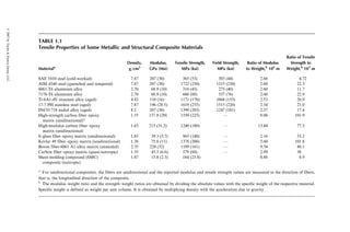
![Apart from these damages, there was no degradation of residual strengths due
to either fatigue or environmental exposure. A good correlation was found
between the on-ground environmental test program and the performance of the
composite components after flight exposure.
Airbus was the first commercial aircraft manufacturer to make extensive
use of composites in their A310 aircraft, which was introduced in 1987. The
composite components weighed about 10% of the aircraft’s weight and
included such components as the lower access panels and top panels of the
wing leading edge, outer deflector doors, nose wheel doors, main wheel leg
fairing doors, engine cowling panels, elevators and fin box, leading and
trailing edges of fins, flap track fairings, flap access doors, rear and forward
wing–body fairings, pylon fairings, nose radome, cooling air inlet fairings, tail
leading edges, upper surface skin panels above the main wheel bay, glide slope
antenna cover, and rudder. The composite vertical stabilizer, which is 8.3 m
high by 7.8 m wide at the base, is about 400 kg lighter than the aluminum
vertical stabilizer previously used [2]. The Airbus A320, introduced in 1988,
was the first commercial aircraft to use an all-composite tail, which includes
the tail cone, vertical stabilizer, and horizontal stabilizer. Figure 1.2 schemat-
ically shows the composite usage in Airbus A380 introduced in 2006. About
25% of its weight is made of composites. Among the major composite com-
ponents in A380 are the central torsion box (which links the left and right
wings under the fuselage), rear-pressure bulkhead (a dome-shaped partition
that separates the passenger cabin from the rear part of the plane that is not
pressurized), the tail, and the flight control surfaces, such as the flaps, spoilers,
and ailerons.
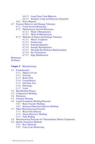
TABLE 1.4
Early Applications of Fiber-Reinforced Polymers in Commercial Aircrafts
Aircraft Component Weight (lb)
Weight
Reduction (%) Comments
Boeing
727 Elevator face sheets 98 25 10 units installed in 1980
737 Horizontal stabilizer 204 22
737 Wing spoilers — 37 Installed in 1973
756 Ailerons, rudders,
elevators, fairings, etc.
3340 (total) 31
McDonnell-Douglas
DC-10 Upper rudder 67 26 13 units installed in 1976
DC-10 Vertical stabilizer 834 17
Lockheed
L-1011 Aileron 107 23 10 units installed in 1981
L-1011 Vertical stabilizer 622 25
ß 2007 by Taylor Francis Group, LLC.](https://image.slidesharecdn.com/fiberreinforcedcompositesmaterialsmanufacturinganddesignp1-220510152925-9ef3de0d/85/Fiber_Reinforced_Composites_Materials_Manufacturing_and_Design_P-1-pdf-26-320.jpg)

![next line of airplanes, called the Boeing 787 Dreamliner, will be made of carbon
fiber-reinforced polymers. The other major materials in Boeing 787 will be
aluminum alloys (20%), titanium alloys (15%), and steel (10%). Two of the
major composite components in 787 will be the fuselage and the forward
section, both of which will use carbon fiber-reinforced epoxy as the major
material of construction.
There are several pioneering examples of using larger quantities of com-
posite materials in smaller aircrafts. One of these examples is the Lear Fan
2100, a business aircraft built in 1983, in which carbon fiber–epoxy and Kevlar
49 fiber–epoxy accounted for ~70% of the aircraft’s airframe weight. The
composite components in this aircraft included wing skins, main spar, fuselage,
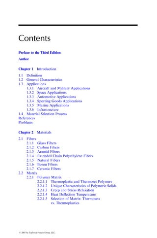
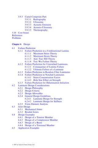
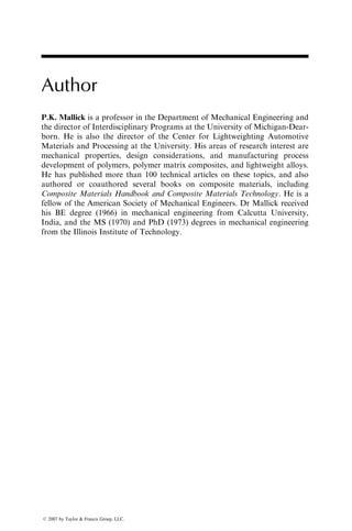
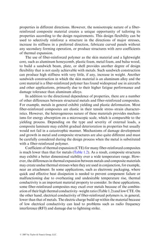
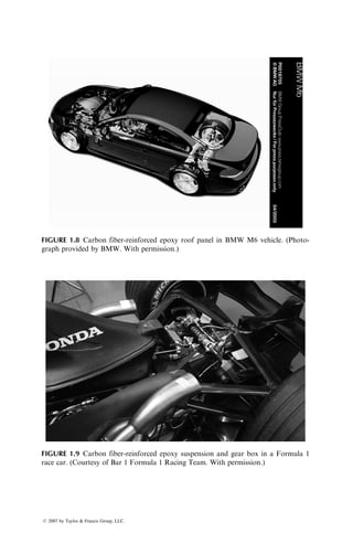
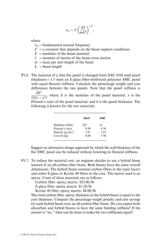
empennage, and various control surfaces [3]. Another example is the Rutan
Voyager (Figure 1.4), which was an all-composite airplane and made the first-
ever nonstop flight around the world in 1986. To travel 25,000 miles without
refueling, the Voyager airplane had to be extremely light and contain as much
fuel as needed.
Fiber-reinforced polymers are used in many military and commercial heli-
copters for making baggage doors, fairings, vertical fins, tail rotor spars, and so
on. One key helicopter application of composite materials is the rotor blades.
Carbon or glass fiber-reinforced epoxy is used in this application. In addition to
significant weight reduction over aluminum, they provide a better control over
the vibration characteristics of the blades. With aluminum, the critical flopping
FIGURE 1.4 Rutan Voyager all-composite plane.
ß 2007 by Taylor Francis Group, LLC.](https://image.slidesharecdn.com/fiberreinforcedcompositesmaterialsmanufacturinganddesignp1-220510152925-9ef3de0d/85/Fiber_Reinforced_Composites_Materials_Manufacturing_and_Design_P-1-pdf-28-320.jpg)
![and twisting frequencies are controlled principally by the classical method of
mass distribution [4]. With fiber-reinforced polymers, they can also be con-
trolled by varying the type, concentration, distribution, as well as orientation of
fibers along the blade’s chord length. Another advantage of using fiber-
reinforced polymers in blade applications is the manufacturing flexibility of
these materials. The composite blades can be filament-wound or molded into
complex airfoil shapes with little or no additional manufacturing costs, but
conventional metal blades are limited to shapes that can only be extruded,
machined, or rolled.
The principal reason for using fiber-reinforced polymers in aircraft and
helicopter applications is weight saving, which can lead to significant fuel
saving and increase in payload. There are several other advantages of using
them over aluminum and titanium alloys.
1. Reduction in the number of components and fasteners, which results in
a reduction of fabrication and assembly costs. For example, the vertical
fin assembly of the Lockheed L-1011 has 72% fewer components and
83% fewer fasteners when it is made of carbon fiber-reinforced epoxy
than when it is made of aluminum. The total weight saving is 25.2%.
2. Higher fatigue resistance and corrosion resistance, which result in a
reduction of maintenance and repair costs. For example, metal fins
used in helicopters flying near ocean coasts use an 18 month repair
cycle for patching corrosion pits. After a few years in service, the
patches can add enough weight to the fins to cause a shift in the center
of gravity of the helicopter, and therefore the fin must then be rebuilt or
replaced. The carbon fiber-reinforced epoxy fins do not require any
repair for corrosion, and therefore, the rebuilding or replacement cost
is eliminated.
3. The laminated construction used with fiber-reinforced polymers allows
the possibility of aeroelastically tailoring the stiffness of the airframe
structure. For example, the airfoil shape of an aircraft wing can be
controlled by appropriately adjusting the fiber orientation angle in
each lamina and the stacking sequence to resist the varying lift and
drag loads along its span. This produces a more favorable airfoil
shape and enhances the aerodynamic characteristics critical to the air-
craft’s maneuverability.
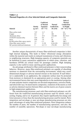
The key limiting factors in using carbon fiber-reinforced epoxy in aircraft
structures are their high cost, relatively low impact damage tolerance (from
bird strikes, tool drop, etc.), and susceptibility to lightning damage. When they
are used in contact with aluminum or titanium, they can induce galvanic
corrosion in the metal components. The protection of the metal components
from corrosion can be achieved by coating the contacting surfaces with a
corrosion-inhibiting paint, but it is an additional cost.
ß 2007 by Taylor Francis Group, LLC.](https://image.slidesharecdn.com/fiberreinforcedcompositesmaterialsmanufacturinganddesignp1-220510152925-9ef3de0d/85/Fiber_Reinforced_Composites_Materials_Manufacturing_and_Design_P-1-pdf-29-320.jpg)
![1.3.2 SPACE APPLICATIONS
Weight reduction is the primary reason for using fiber-reinforced composites in
many space vehicles [5]. Among the various applications in the structure of
space shuttles are the mid-fuselage truss structure (boron fiber-reinforced alu-
minum tubes), payload bay door (sandwich laminate of carbon fiber-reinforced
epoxy face sheets and aluminum honeycomb core), remote manipulator arm
(ultrahigh-modulus carbon fiber-reinforced epoxy tube), and pressure vessels
(Kevlar 49 fiber-reinforced epoxy).
In addition to the large structural components, fiber-reinforced polymers are
used for support structures for many smaller components, such as solar arrays,
antennas, optical platforms, and so on [6]. A major factor in selecting them for
these applications is their dimensional stability over a wide temperature range.
Many carbon fiber-reinforced epoxy laminates can be ‘‘designed’’ to produce a
CTE close to zero. Many aerospace alloys (e.g., Invar) also have a comparable
CTE. However, carbon fiber composites have a much lower density, higher
strength, as well as a higher stiffness–weight ratio. Such a unique combination
of mechanical properties and CTE has led to a number of applications for carbon
fiber-reinforced epoxies in artificial satellites. One such application is found in
the support structure for mirrors and lenses in the space telescope [7]. Since the
temperature in space may vary between 1008C and 1008C, it is critically
important that the support structure be dimensionally stable; otherwise, large
changes in the relative positions of mirrors or lenses due to either thermal
expansion or distortion may cause problems in focusing the telescope.
Carbon fiber-reinforced epoxy tubes are used in building truss structures for
low earth orbit (LEO) satellites and interplanetary satellites. These truss structures
support optical benches, solar array panels, antenna reflectors, and other modules.
Carbon fiber-reinforced epoxies are preferred over metals or metal matrix com-
posites because of their lower weight as well as very low CTE. However, one of the
major concerns with epoxy-based composites in LEO satellites is that they are
susceptible to degradation due to atomic oxygen (AO) absorption from the
earth’s rarefied atmosphere. This problem is overcome by protecting the tubes
from AO exposure, for example, by wrapping them with thin aluminum foils.
Other concerns for using fiber-reinforced polymers in the space environ-
ment are the outgassing of the polymer matrix when they are exposed to
vacuum in space and embrittlement due to particle radiation. Outgassing can
cause dimensional changes and embrittlement may lead to microcrack forma-
tion. If the outgassed species are deposited on the satellite components, such as
sensors or solar cells, their function may be seriously degraded [8].
1.3.3 AUTOMOTIVE APPLICATIONS
Applications of fiber-reinforced composites in the automotive industry can be
classified into three groups: body components, chassis components, and engine
ß 2007 by Taylor Francis Group, LLC.](https://image.slidesharecdn.com/fiberreinforcedcompositesmaterialsmanufacturinganddesignp1-220510152925-9ef3de0d/85/Fiber_Reinforced_Composites_Materials_Manufacturing_and_Design_P-1-pdf-30-320.jpg)
![radiator support is typically made of two SMC parts bonded together by an
adhesive instead of 20 or more steel parts assembled together by large number
of screws. The material in the composite radiator support is randomly oriented
discontinuous E-glass fiber-reinforced vinyl ester. Another example of parts
integration can be found in the station wagon tailgate assembly [9], which has
significant load-bearing requirements in the open position. The composite
tailgate consists of two pieces, an outer SMC shell and an inner reinforcing
SMC piece. They are bonded together using a urethane adhesive. The compos-
ite tailgate replaces a seven-piece steel tailgate assembly, at about one-third its
weight. The material for both the outer shell and the inner reinforcement is a
randomly oriented discontinuous E-glass fiber-reinforced polyester.
Another manufacturing process for making composite body panels in the
automotive industry is called the structural reaction injection molding (SRIM).
The fibers in these parts are usually randomly oriented discontinuous E-glass
fibers and the matrix is a polyurethane or polyurea. Figure 1.7 shows the
photograph of a one-piece 2 m long cargo box that is molded using this process.
The wall thickness of the SRIM cargo box is 3 mm and its one-piece construc-
tion replaces four steel panels that are joined together using spot welds.
Among the chassis components, the first major structural application of
fiber-reinforced composites is the Corvette rear leaf spring, introduced first in
FIGURE 1.6 Compression-molded SMC valve cover for a truck engine. (Courtesy of
Ashland Chemicals and American Composites Alliance. With permission.)
ß 2007 by Taylor Francis Group, LLC.](https://image.slidesharecdn.com/fiberreinforcedcompositesmaterialsmanufacturinganddesignp1-220510152925-9ef3de0d/85/Fiber_Reinforced_Composites_Materials_Manufacturing_and_Design_P-1-pdf-32-320.jpg)
![1981 [10]. Unileaf E-glass fiber-reinforced epoxy springs have been used to
replace multileaf steel springs with as much as 80% weight reduction. Other
structural chassis components, such as drive shafts and road wheels, have been
successfully tested in laboratories and proving grounds. They have also been
used in limited quantities in production vehicles. They offer opportunities for
substantial weight savings, but so far they have not proven to be cost-effective
over their steel counterparts.
The application of fiber-reinforced composites in engine components has
not been as successful as the body and chassis components. Fatigue loads at
very high temperatures pose the greatest challenge in these applications. Devel-
opment of high-temperature polymers as well as metal matrix or ceramic matrix
composites would greatly enhance the potential for composite usage in this area.
Manufacturing and design of fiber-reinforced composite materials for auto-
motive applications are significantly different from those for aircraft applica-
tions. One obvious difference is in the volume of production, which may range
from 100 to 200 pieces per hour for automotive components compared with a
few hundred pieces per year for aircraft components. Although the labor-
intensive hand layup followed by autoclave molding has worked well for
fabricating aircraft components, high-speed methods of fabrication, such as
compression molding and SRIM, have emerged as the principal manufacturing
process for automotive composites. Epoxy resin is the major polymer matrix
FIGURE 1.7 One-piece cargo box for a pickup truck made by the SRIM process.
ß 2007 by Taylor Francis Group, LLC.](https://image.slidesharecdn.com/fiberreinforcedcompositesmaterialsmanufacturinganddesignp1-220510152925-9ef3de0d/85/Fiber_Reinforced_Composites_Materials_Manufacturing_and_Design_P-1-pdf-33-320.jpg)
![used in aerospace composites; however, the curing time for epoxy resin is very
long, which means the production time for epoxy matrix composites is also
very long. For this reason, epoxy is not considered the primary matrix
material in automotive composites. The polymer matrix used in automotive
applications is either a polyester, a vinyl ester, or polyurethane, all of which
require significantly lower curing time than epoxy. The high cost of carbon
fibers has prevented their use in the cost-conscious automotive industry.
Instead of carbon fibers, E-glass fibers are used in automotive composites
because of their significantly lower cost. Even with E-glass fiber-reinforced
composites, the cost-effectiveness issue has remained particularly critical, since
the basic material of construction in present-day automobiles is low-carbon
steel, which is much less expensive than most fiber-reinforced composites on a
unit weight basis.
Although glass fiber-reinforced polymers are the primary composite mater-
ials used in today’s automobiles, it is well recognized that significant vehicle
weight reduction needed for improved fuel efficiency can be achieved only with
carbon fiber-reinforced polymers, since they have much higher strength–weight
and modulus–weight ratios. The problem is that the current carbon fiber price,
at $16=kg or higher, is not considered cost-effective for automotive applica-
tions. Nevertheless, many attempts have been made in the past to manufacture
structural automotive parts using carbon fiber-reinforced polymers; unfortu-
nately most of them did not go beyond the stages of prototyping and structural
testing. Recently, several high-priced vehicles have started using carbon fiber-
reinforced polymers in a few selected components. One recent example of this is
seen in the BMW M6 roof panel (Figure 1.8), which was produced by a process
called resin transfer molding (RTM). This panel is twice as thick as a compar-
able steel panel, but 5.5 kg lighter. One added benefit of reducing the weight of
the roof panel is that it slightly lowers the center of gravity of the vehicle, which
is important for sports coupe.
Fiber-reinforced composites have become the material of choice in motor
sports where lightweight structure is used for gaining competitive advantage of
higher speed [11] and cost is not a major material selection decision factor. The
first major application of composites in race cars was in the 1950s when glass
fiber-reinforced polyester was introduced as replacement for aluminum body
panels. Today, the composite material used in race cars is mostly carbon fiber-
reinforced epoxy. All major body, chassis, interior, and suspension components
in today’s Formula 1 race cars use carbon fiber-reinforced epoxy. Figure 1.9
shows an example of carbon fiber-reinforced composite used in the gear box
and rear suspension of a Formula 1 race car. One major application of carbon
fiber-reinforced epoxy in Formula 1 cars is the survival cell, which protects the
driver in the event of a crash. The nose cone located in front of the survival cell
is also made of carbon fiber-reinforced epoxy. Its controlled crush behavior is
also critical to the survival of the driver.
ß 2007 by Taylor Francis Group, LLC.](https://image.slidesharecdn.com/fiberreinforcedcompositesmaterialsmanufacturinganddesignp1-220510152925-9ef3de0d/85/Fiber_Reinforced_Composites_Materials_Manufacturing_and_Design_P-1-pdf-34-320.jpg)
![1.3.4 SPORTING GOODS APPLICATIONS
Fiber-reinforced polymers are extensively used in sporting goods ranging
from tennis rackets to athletic shoes (Table 1.5) and are selected over such
traditional materials as wood, metals, and leather in many of these applications
[12]. The advantages of using fiber-reinforced polymers are weight reduction,
vibration damping, and design flexibility. Weight reduction achieved by substi-
tuting carbon fiber-reinforced epoxies for metals leads to higher speeds and
quick maneuvering in competitive sports, such as bicycle races and canoe races.
In some applications, such as tennis rackets or snow skis, sandwich construc-
tions of carbon or boron fiber-reinforced epoxies as the skin material and a
soft, lighter weight urethane foam as the core material produces a higher weight
reduction without sacrificing stiffness. Faster damping of vibrations provided
by fiber-reinforced polymers reduces the shock transmitted to the player’s arm
in tennis or racket ball games and provides a better ‘‘feel’’ for the ball. In
archery bows and pole-vault poles, the high stiffness–weight ratio of fiber-
reinforced composites is used to store high elastic energy per unit weight, which
helps in propelling the arrow over a longer distance or the pole-vaulter to jump
a greater height. Some of these applications are described later.
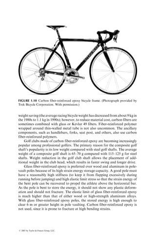
Bicycle frames for racing bikes today are mostly made of carbon fiber-
reinforced epoxy tubes, fitted together by titanium fittings and inserts. An
example is shown in Figure 1.10. The primary purpose of using carbon fibers is
TABLE 1.5
Applications of Fiber-Reinforced Polymers
in Sporting Goods
Tennis rackets
Racket ball rackets
Golf club shafts
Fishing rods
Bicycle frames
Snow and water skis
Ski poles, pole vault poles
Hockey sticks
Baseball bats
Sail boats and kayaks
Oars, paddles
Canoe hulls
Surfboards, snow boards
Arrows
Archery bows
Javelins
Helmets
Exercise equipment
Athletic shoe soles and heels
ß 2007 by Taylor Francis Group, LLC.](https://image.slidesharecdn.com/fiberreinforcedcompositesmaterialsmanufacturinganddesignp1-220510152925-9ef3de0d/85/Fiber_Reinforced_Composites_Materials_Manufacturing_and_Design_P-1-pdf-36-320.jpg)
![Glass and carbon fiber-reinforced epoxy fishing rods are very common
today, even though traditional materials, such as bamboo, are still used. For
fly-fishing rods, carbon fiber-reinforced epoxy is preferred, since it produces a
smaller tip deflection (because of its higher modulus) and ‘‘wobble-free’’ action
during casting. It also dampens the vibrations more rapidly and reduces the
transmission of vibration waves along the fly line. Thus, the casting can be
longer, quieter, and more accurate, and the angler has a better ‘‘feel’’ for the
catch. Furthermore, carbon fiber-reinforced epoxy rods recover their original
shape much faster than the other rods. A typical carbon fiber-reinforced epoxy
rod of No. 6 or No. 7 line weighs only 37 g. The lightness of these rods is also a
desirable feature to the anglers.
1.3.5 MARINE APPLICATIONS
Glass fiber-reinforced polyesters have been used in different types of boats (e.g.,
sail boats, fishing boats, dinghies, life boats, and yachts) ever since their
introduction as a commercial material in the 1940s [13]. Today, nearly 90% of
all recreational boats are constructed of either glass fiber-reinforced polyester or
glass fiber-reinforced vinyl ester resin. Among the applications are hulls, decks,
and various interior components. The manufacturing process used for making a
majority of these components is called contact molding. Even though it is
a labor-intensive process, the equipment cost is low, and therefore it is afford-
able to many of the small companies that build these boats. In recent years,
Kevlar 49 fiber is replacing glass fibers in some of these applications because of its
higher tensile strength–weight and modulus–weight ratios than those of glass
fibers. Among the application areas are boat hulls, decks, bulkheads, frames,
masts, and spars. The principal advantage is weight reduction, which translates
into higher cruising speed, acceleration, maneuverability, and fuel efficiency.
Carbon fiber-reinforced epoxy is used in racing boats in which weight
reduction is extremely important for competitive advantage. In these boats,
the complete hull, deck, mast, keel, boom, and many other structural compon-
ents are constructed using carbon fiber-reinforced epoxy laminates and sand-
wich laminates of carbon fiber-reinforced epoxy skins with either honeycomb
core or plastic foam core. Carbon fibers are sometimes hybridized with other
lower density and higher strain-to-failure fibers, such as high-modulus poly-
ethylene fibers, to improve impact resistance and reduce the boat’s weight.
The use of composites in naval ships started in the 1950s and has grown
steadily since then [14]. They are used in hulls, decks, bulkheads, masts,
propulsion shafts, rudders, and others of mine hunters, frigates, destroyers,
and aircraft carriers. Extensive use of fiber-reinforced polymers can be seen in
Royal Swedish Navy’s 72 m long, 10.4 m wide Visby-class corvette, which is the
largest composite ship in the world today. Recently, the US navy has commis-
sioned a 24 m long combat ship, called Stiletto, in which carbon fiber-
reinforced epoxy will be the primary material of construction. The selection
ß 2007 by Taylor Francis Group, LLC.](https://image.slidesharecdn.com/fiberreinforcedcompositesmaterialsmanufacturinganddesignp1-220510152925-9ef3de0d/85/Fiber_Reinforced_Composites_Materials_Manufacturing_and_Design_P-1-pdf-38-320.jpg)
![of carbon fiber-reinforced epoxy is based on the design requirements of light-
weight and high strength needed for high speed, maneuverability, range, and
payload capacity of these ships. Their stealth characteristics are also important
in minimizing radar reflection.
1.3.6 INFRASTRUCTURE
Fiber-reinforced polymers have a great potential for replacing reinforced con-
crete and steel in bridges, buildings, and other civil infrastructures [15]. The
principal reason for selecting these composites is their corrosion resistance,
which leads to longer life and lower maintenance and repair costs. Reinforced
concrete bridges tend to deteriorate after several years of use because of
corrosion of steel-reinforcing bars (rebars) used in their construction. The
corrosion problem is exacerbated because of deicing salt spread on the bridge
road surface in winter months in many parts of the world. The deterioration
can become so severe that the concrete surrounding the steel rebars can start to
crack (due to the expansion of corroding steel bars) and ultimately fall off, thus
weakening the structure’s load-carrying capacity. The corrosion problem does
not exist with fiber-reinforced polymers. Another advantage of using fiber-
reinforced polymers for large bridge structures is their lightweight, which
means lower dead weight for the bridge, easier transportation from the pro-
duction factory (where the composite structure can be prefabricated) to the
bridge location, easier hauling and installation, and less injuries to people in
case of an earthquake. With lightweight construction, it is also possible to
design bridges with longer span between the supports.
One of the early demonstrations of a composite traffic bridge was made in
1995 by Lockheed Martin Research Laboratories in Palo Alto, California. The
bridge deck was a 9 m long 3 5.4 m wide quarter-scale section and the material
selected was E-glass fiber-reinforced polyester. The composite deck was a
sandwich laminate of 15 mm thick E-glass fiber-reinforced polyester face sheets
and a series of E-glass fiber-reinforced polyester tubes bonded together to form
the core. The deck was supported on three U-shaped beams made of E-glass
fabric-reinforced polyester. The design was modular and the components were
stackable, which simplified both their transportation and assembly.
In recent years, a number of composite bridge decks have been constructed
and commissioned for service in the United States and Canada. The Wickwire
Run Bridge located in West Virginia, United States is an example of one such
construction. It consists of full-depth hexagonal and half-depth trapezoidal
profiles made of glass fabric-reinforced polyester matrix. The profiles are
supported on steel beams. The road surface is a polymer-modified concrete.
Another example of a composite bridge structure is shown in Figure 1.11,
which replaced a 73 year old concrete bridge with steel rebars. The replacement
was necessary because of the severe deterioration of the concrete deck, which
reduced its load rating from 10 to only 4.3 t and was posing safety concerns. In
ß 2007 by Taylor Francis Group, LLC.](https://image.slidesharecdn.com/fiberreinforcedcompositesmaterialsmanufacturinganddesignp1-220510152925-9ef3de0d/85/Fiber_Reinforced_Composites_Materials_Manufacturing_and_Design_P-1-pdf-39-320.jpg)
![the composite bridge, the internal reinforcement for the concrete deck is a two-
layer construction and consists primarily of pultruded I-section bars (I-bars) in
the width direction (perpendicular to the direction of traffic) and pultruded
round rods in the length directions. The material for the pultruded sections is
glass fiber-reinforced vinyl ester. The internal reinforcement is assembled by
inserting the round rods through the predrilled holes in I-bar webs and keeping
them in place by vertical connectors.
Besides new bridge construction or complete replacement of reinforced
concrete bridge sections, fiber-reinforced polymer is also used for upgrading,
retrofitting, and strengthening damaged, deteriorating, or substandard concrete
or steel structures [16]. For upgrading, composite strips and plates are
attached in the cracked or damaged areas of the concrete structure using adhe-
sive, wet layup, or resin infusion. Retrofitting of steel girders is accomplished
View from the top showing round
composite cross-rods inserted in the
predrilled holes in composite I-bars
placed in the direction of trafffic
FIGURE 1.11 Glass fiber-reinforced vinyl ester pultruded sections in the construction of
a bridge deck system. (Photograph provided by Strongwell Corporation. With permission.)
ß 2007 by Taylor Francis Group, LLC.](https://image.slidesharecdn.com/fiberreinforcedcompositesmaterialsmanufacturinganddesignp1-220510152925-9ef3de0d/85/Fiber_Reinforced_Composites_Materials_Manufacturing_and_Design_P-1-pdf-40-320.jpg)
![application of the load. If, on the other hand, there is a possibility of brittle
failure because of the influence of the operating environmental conditions,
fracture toughness is the material property to consider.
In many designs the performance requirement may include stiffness, which
is defined as load per unit deformation. Stiffness should not be confused with
modulus, since stiffness depends not only on the modulus of the material
(which is a material property), but also on the design. For example, the stiffness
of a straight beam with solid circular cross section depends not only on the
modulus of the material, but also on its length, diameter, and how it is
supported (i.e., boundary conditions). For a given beam length and support
conditions, the stiffness of the beam with solid circular cross section is propor-
tional to Ed 4
, where E is the modulus of the beam material and d is its diameter.
Therefore, the stiffness of this beam can be increased by either selecting a higher
modulus material, or increasing the diameter, or doing both. Increasing the
diameter is more effective in increasing the stiffness, but it also increases
the weight and cost of the beam. In some designs, it may be possible to increase
the beam stiffness by incorporating other design features, such as ribs, or by
using a sandwich construction.
In designing structures with minimum mass or minimum cost, material
properties must be combined with mass density (r), cost per unit mass ($=kg),
and so on. For example, if the design objective for a tension linkage or a tie bar
is to meet the stiffness performance criterion with minimum mass, the material
selection criterion involves not just the tensile modulus of the material (E), but
also the modulus–density ratio (E=r). The modulus–density ratio is a material
index, and the material that produces the highest value of this material index
should be selected for minimum mass design of the tension link. The material
index depends on the application and the design objective. Table 1.6 lists the
material indices for minimum mass design of a few simple structures.
As an example of the use of the material index in preliminary material
selection, consider the carbon fiber–epoxy quasi-isotropic laminate in Table 1.1.
Thin laminates of this type are considered well-suited for many aerospace
applications [1], since they exhibit equal elastic properties (e.g., modulus) in
all directions in the plane of load application. The quasi-isotropic laminate
in Table 1.1 has an elastic modulus of 45.5 GPa, which is 34% lower than that
of the 7178-T6 aluminum alloy and 59% lower than that of the Ti-6 Al-4V
titanium alloy. The aluminum and the titanium alloys are the primary metallic
alloys used in the construction of civilian and military aircrafts. Even though
the quasi-isotropic carbon fiber–epoxy composite laminate has a lower modulus,
it is a good candidate for substituting the metallic alloys in stiffness-critical
aircraft structures. This is because the carbon fiber–epoxy quasi-isotropic
laminate has a superior material index in minimum mass design of stiffness-
critical structures. This can be easily verified by comparing the values of
the material index E1=3
r of all three materials, assuming that the structure can
be modeled as a thin plate under bending load.
ß 2007 by Taylor Francis Group, LLC.](https://image.slidesharecdn.com/fiberreinforcedcompositesmaterialsmanufacturinganddesignp1-220510152925-9ef3de0d/85/Fiber_Reinforced_Composites_Materials_Manufacturing_and_Design_P-1-pdf-42-320.jpg)
![Weight reduction is often the principal consideration for selecting fiber-
reinforced polymers over metals, and for many applications, they provide a
higher material index than metals, and therefore, suitable for minimum mass
design. Depending on the application, there are other advantages of using fiber-
reinforced composites, such as higher damping, no corrosion, parts integration,
control of thermal expansion, and so on, that should be considered as well, and
some of these advantages add value to the product that cannot be obtained
with metals. One great advantage is the tailoring of properties according to the
design requirements, which is demonstrated in the example of load-bearing
orthopedic implants [17]. One such application is the bone plate used for bone
fracture fixation. In this application, the bone plate is attached to the bone
fracture site with screws to hold the fractured pieces in position, reduce the
mobility at the fracture interface, and provide the required stress-shielding of
the bone for proper healing. Among the biocompatible materials used for
orthopedic implants, stainless steel and titanium are the two most common
materials used for bone plates. However, the significantly higher modulus of
both of these materials than that of bone creates excessive stress-shielding, that is,
they share the higher proportion of the compressive stresses during healing than
the bone. The advantage of using fiber-reinforced polymers is that they can be
designed to match the modulus of bone, and indeed, this is the reason for
TABLE 1.6
Material Index for Stiffness and Strength-Critical Designs at Minimum Mass
Structure Constraints
Design
Variable
Material Index
Stiffness-Critical
Design
Strength-Critical
Design
Round tie bar loaded
in axial tension
Length fixed Diameter
E
r
Sf
r
Rectangular beam loaded
in bending
Length and
width fixed
Height
E1=3
r
S
1=2
f
r
Round bar or shaft loaded
in torsion
Length fixed Diameter
G1=2
r
S
2=3
f
r
Flat plate loaded in
bending
Length and
width fixed
Thickness
E1=3
r
S
1=2
f
r
Round column loaded
in compression
Length Diameter
E1=2
r
Sf
r
Source: Adapted from Ashby, M.F., Material Selection in Mechanical Design, 3rd Ed., Elsevier,
Oxford, UK, 2005.
Note: r ¼ mass density, E ¼ Young’s modulus, G ¼ shear modulus, and Sf ¼ strength.
ß 2007 by Taylor Francis Group, LLC.](https://image.slidesharecdn.com/fiberreinforcedcompositesmaterialsmanufacturinganddesignp1-220510152925-9ef3de0d/85/Fiber_Reinforced_Composites_Materials_Manufacturing_and_Design_P-1-pdf-43-320.jpg)
![selecting carbon fiber-reinforced epoxy or polyether ether ketone (PEEK) for
such an application [18,19].
REFERENCES
1. C.E. Harris, J.H. Starnes, Jr., and M.J. Shuart, Design and manufacturing of
aerospace composite structures, state-of-the-art assessment, J. Aircraft, 39:545
(2002).
2. C. Soutis, Carbon fiber reinforced plastics in aircraft applications, Mater. Sci. Eng.,
A, 412:171 (2005).
3. J.V. Noyes, Composites in the construction of the Lear Fan 2100 aircraft, Compos-
ites, 14:129 (1983).
4. R.L. Pinckney, Helicopter rotor blades, Appl. Composite Mat., ASTM STP, 524:108
(1973).
5. N.R. Adsit, Composites for space applications, ASTM Standardization News,
December (1983).
6. H. Bansemir and O. Haider, Fibre composite structures for space applications—recent
and future developments, Cryogenics, 38:51 (1998).
7. E.G. Wolff, Dimensional stability of structural composites for spacecraft applica-
tions, Metal Prog., 115:54 (1979).
8. J. Guthrie, T.B. Tolle, and D.H. Rose, Composites for orbiting platforms, AMP-
TIAC Q., 8:51 (2004).
9. D.A. Riegner, Composites in the automotive industry, ASTM Standardization
News, December (1983).
10. P. Beardmore, Composite structures for automobiles, Compos. Struct., 5:163 (1986).
11. G. Savage, Composite materials in Formula 1 racing, Metals Mater., 7:617 (1991).
12. V.P. McConnell, Application of composites in sporting goods, Comprehensive Com-
posite Materials, Vol. 6, Elsevier, Amsterdam, pp. 787–809 (2000).
13. W. Chalmers, The potential for the use of composite materials in marine structures,
Mar. Struct., 7:441 (1994).
14. A.P. Mouritz, E. Gellert, P. Burchill, and K. Challis, Review of advanced composite
structures for naval ships and submarines, Compos. Struct., 53:21 (2001).
15. L.C. Hollaway, The evolution of and the way forward for advanced polymer
composites in the civil infrastructure, Construct. Build. Mater., 17:365 (2003).
16. V.M. Karbhari, Fiber reinforced composite bridge systems—transition from the
laboratory to the field, Compos. Struct., 66:5 (2004).
17. S.L. Evans and P.J. Gregson, Composite technology in load-bearing orthopedic
implants, Biomaterials, 19:1329 (1998).
18. M.S. Ali, T.A. French, G.W. Hastings, T. Rae, N. Rushton, E.R.S. Ross, and
C.H. Wynn-Jones, Carbon fibre composite bone plates, J. Bone Joint Surg.,
72-B:586 (1990).
19. Z.-M. Huang and K. Fujihara, Stiffness and strength design of composite bone
plate, Compos. Sci. Tech., 65:73 (2005).
ß 2007 by Taylor Francis Group, LLC.](https://image.slidesharecdn.com/fiberreinforcedcompositesmaterialsmanufacturinganddesignp1-220510152925-9ef3de0d/85/Fiber_Reinforced_Composites_Materials_Manufacturing_and_Design_P-1-pdf-44-320.jpg)

![fractures. From the load-time record of the test, the following tensile properties
are determined:
Tensile strength sfu ¼
Fu
Af
(2:1)
and
Tensile modulus Ef ¼
Lf
CAf
, (2:2)
where
Fu ¼ force at failure
Af ¼ average filament cross-sectional area, measured by a planimeter from
the photomicrographs of filament ends
Lf ¼ gage length
C ¼ true compliance, determined from the chart speed, loading rate, and
the system compliance
Tensile stress–strain diagrams obtained from single filament test of reinforcing
fibers in use are almost linear up to the point of failure, as shown in Figure 2.5.
They also exhibit very low strain-to-failure and a brittle failure mode. Although
the absence of yielding does not reduce the load-carrying capacity of the fibers,
it does make them prone to damage during handling as well as during contact
with other surfaces. In continuous manufacturing operations, such as filament
winding, frequent fiber breakage resulting from such damages may slow the
rate of production.
The high tensile strengths of the reinforcing fibers are generally attributed
to their filamentary form in which there are statistically fewer surface flaws than
in the bulk form. However, as in other brittle materials, their tensile strength
data exhibit a large amount of scatter. An example is shown in Figure 2.6.
The experimental strength variation of brittle filaments is modeled using the
following Weibull distribution function [1]:
f (sfu) ¼ asa
o sa1
fu
Lf
Lo
exp
Lf
Lo
sfu
so
a
, (2:3)
where
f(sfu) ¼ probability of filament failure at a stress level equal to sfu
sfu ¼ filament strength
Lf ¼ filament length
Lo ¼ reference length
a ¼ shape parameter
so ¼ scale parameter (the filament strength at Lf ¼ Lo)
ß 2007 by Taylor Francis Group, LLC.](https://image.slidesharecdn.com/fiberreinforcedcompositesmaterialsmanufacturinganddesignp1-220510152925-9ef3de0d/85/Fiber_Reinforced_Composites_Materials_Manufacturing_and_Design_P-1-pdf-55-320.jpg)
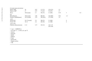
![The mean filament strength fu is given by
sfu ¼ so
Lf
Lo
1=a
G 1 þ
1
a
, (2:5)
where G represents a gamma function. Equation 2.5 clearly shows that the
mean strength of a brittle filament decreases with increasing length. This is also
demonstrated in Figure 2.7.
Tensile properties of fibers can also be determined using fiber bundles. It has
been observed that even though the tensile strength distribution of individual
filaments follows the Weibull distribution, the tensile strength distribution of
fiber bundles containing a large number of parallel filaments follows a normal
distribution [1]. The maximum strength, sfm, that the filaments in the bundle will
exhibit and the mean bundle strength, b, can be expressed in terms of the Weibull
parameters determined for individual filaments. They are given as follows:
sfm ¼ so
Lf
Lo
a
1=a
,
sb ¼ so
Lf
Lo
a
1=a
e1=a
: (2:6)
20
(a)
MODMOR I
Carbon fiber
(b)
GY-70
Carbon fiber
Frequency
Frequency
10
0
20
10
0
100 200 300 400 500 ksi
MPa
690 1380 2070
Tensile strength
2760 3450
FIGURE 2.6 Histograms of tensile strengths for (a) Modmor I carbon fibers and (b)
GY-70 carbon fibers. (After McMahon, P.E., Analysis of the Test Methods for High
Modulus Fibers and Composites, ASTM STP, 521, 367, 1973.)
ß 2007 by Taylor Francis Group, LLC.](https://image.slidesharecdn.com/fiberreinforcedcompositesmaterialsmanufacturinganddesignp1-220510152925-9ef3de0d/85/Fiber_Reinforced_Composites_Materials_Manufacturing_and_Design_P-1-pdf-57-320.jpg)
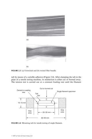
![The fiber bundle test method is similar to the single filament test method. The
fiber bundle can be tested either in dry or resin-impregnated condition. Gener-
ally, the average tensile strength and modulus of fiber bundles are lower than
those measured on single filaments. Figure 2.8 shows the stress–strain diagram
of a dry glass fiber bundle containing 3000 filaments. Even though a single glass
filament shows a linear tensile stress–strain diagram until failure, the glass fiber
strand shows not only a nonlinear stress–strain diagram before reaching the
maximum stress, but also a progressive failure after reaching the maximum
stress. Both nonlinearity and progressive failure occur due to the statistical
distribution of the strength of glass filaments. The weaker filaments in the
bundle fail at low stresses, and the surviving filaments continue to carry the
tensile load; however, the stress in each surviving filament becomes higher.
Some of them fail as the load is increased. After the maximum stress is reached,
the remaining surviving filaments continue to carry even higher stresses and
start to fail, but not all at one time, thus giving the progressive failure mode as
seen in Figure 2.8. Similar tensile stress–strain diagrams are observed with
carbon and other fibers in fiber bundle tests.
In addition to tensile properties, compressive properties of fibers are also of
interest in many applications. Unlike the tensile properties, the compressive
properties cannot be determined directly by simple compression tests on fila-
ments or strands. Various indirect methods have been used to determine the
compressive strength of fibers [2]. One such method is the loop test in which a
filament is bent into the form of a loop until it fails. The compressive strength
600 4140
2760
1380
690
500
400
300
Filament
tensile
strength
(10
3
psi)
Filament
tensile
strength
(MPa)
200
100
50 100 200
(x) Corresponds to 1 in. (25.4 mm) gage length
500
Gage length/filament diameter ratio (10−4
)
1000 2000
Boron
High-strength carbon
Kevlar 49
S-glass
E-glass
5000
FIGURE 2.7 Filament strength variation as a function of gage length-to-diameter ratio.
(After Kevlar 49 Data Manual, E. I. duPont de Nemours Co., 1975.)
ß 2007 by Taylor Francis Group, LLC.](https://image.slidesharecdn.com/fiberreinforcedcompositesmaterialsmanufacturinganddesignp1-220510152925-9ef3de0d/85/Fiber_Reinforced_Composites_Materials_Manufacturing_and_Design_P-1-pdf-58-320.jpg)

![equipment, tends to reduce it to values that are in the range of 1.72–2.07 GPa
(250,000–300,000 psi). Strength degradation is increased as the surface flaws
grow under cyclic loads, which is one of the major disadvantages of using glass
fibers in fatigue applications. Surface compressive stresses obtained by alkali
ion exchange [3] or elimination of surface flaws by chemical etching may reduce
the problem; however, commercial glass fibers are not available with any such
surface modifications.
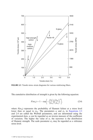
The tensile strength of glass fibers is also reduced in the presence of water or
under sustained loads (static fatigue). Water bleaches out the alkalis from the
surface and deepens the surface flaws already present in fibers. Under sustained
loads, the growth of surface flaws is accelerated owing to stress corrosion by
atmospheric moisture. As a result, the tensile strength of glass fibers is
decreased with increasing time of load duration (Figure 2.11).
2.1.2 CARBON FIBERS
Carbon fibers are commercially available with a variety of tensile modulus
values ranging from 207 GPa (30 3 106
psi) on the low side to 1035 GPa
(150 3 106
psi) on the high side. In general, the low-modulus fibers have
lower density, lower cost, higher tensile and compressive strengths, and higher
tensile strains-to-failure than the high-modulus fibers. Among the advantages
of carbon fibers are their exceptionally high tensile strength–weight ratios as
well as tensile modulus–weight ratios, very low coefficient of linear thermal
expansion (which provides dimensional stability in such applications as space
antennas), high fatigue strengths, and high thermal conductivity (which is even
500
Tensile
stress
(10
3
psi)
24⬚C (75⬚F)
400⬚C (750⬚F)
500⬚C (930⬚F)
600⬚C (1,110⬚F)
400
300
200
100
0
1 10 100
Load duration (min)
Tensile
stress
(MPa)
1,000 10,000
2,760
1,380
0
FIGURE 2.11 Reduction of tensile stress in E-glass fibers as a function of time at various
temperatures. (After Otto, W.H., Properties of glass fibers at elevated temperatures,
Owens Corning Fiberglas Corporation, AD 228551, 1958.)
ß 2007 by Taylor Francis Group, LLC.](https://image.slidesharecdn.com/fiberreinforcedcompositesmaterialsmanufacturinganddesignp1-220510152925-9ef3de0d/85/Fiber_Reinforced_Composites_Materials_Manufacturing_and_Design_P-1-pdf-64-320.jpg)
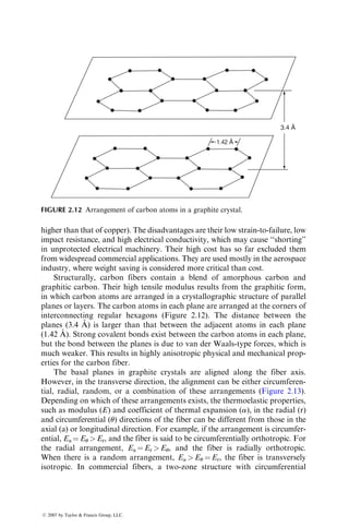
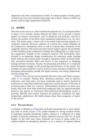
![arrangement in the skin and either radial or random arrangement in the core is
commonly observed [4].
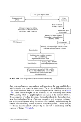
Carbon fibers are manufactured from two types of precursors (starting
materials), namely, textile precursors and pitch precursors. The manufacturing
process from both precursors is outlined in Figure 2.14. The most common
textile precursor is polyacrylonitrile (PAN). The molecular structure of PAN,
illustrated schematically in Figure 2.15a, contains highly polar CN groups that
are randomly arranged on either side of the chain. Filaments are wet spun from
a solution of PAN and stretched at an elevated temperature during which the
polymer chains are aligned in the filament direction. The stretched filaments are
then heated in air at 2008C–3008C for a few hours. At this stage, the CN groups
located on the same side of the original chain combine to form a more stable
and rigid ladder structure (Figure 2.15b), and some of the CH2 groups are
oxidized. In the next step, PAN filaments are carbonized by heating them at a
controlled rate at 10008C–20008C in an inert atmosphere. Tension is main-
tained on the filaments to prevent shrinking as well as to improve molecular
orientation. With the elimination of oxygen and nitrogen atoms, the filaments
now contain mostly carbon atoms, arranged in aromatic ring patterns in
parallel planes. However, the carbon atoms in the neighboring planes are not
yet perfectly ordered, and the filaments have a relatively low tensile modulus.
As the carbonized filaments are subsequently heat-treated at or above 20008C,
(a) (b) (c)
(d) (e)
FIGURE 2.13 Arrangement of graphite crystals in a direction transverse to the fiber
axis: (a) circumferential, (b) radial, (c) random, (d) radial–circumferential, and (e)
random–circumferential.
ß 2007 by Taylor Francis Group, LLC.](https://image.slidesharecdn.com/fiberreinforcedcompositesmaterialsmanufacturinganddesignp1-220510152925-9ef3de0d/85/Fiber_Reinforced_Composites_Materials_Manufacturing_and_Design_P-1-pdf-66-320.jpg)
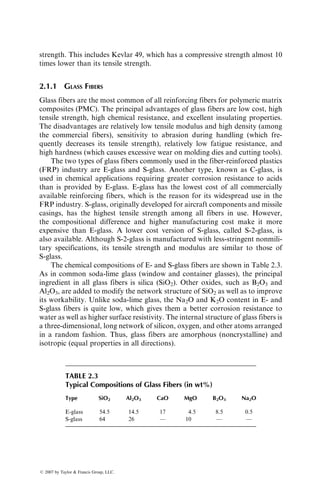
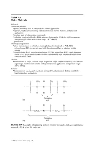
![lowest modulus, while the ultrahigh-modulus PAN carbon fibers, such as
GY-70, have the lowest tensile strength as well as the lowest tensile strain-
to-failure. A number of intermediate modulus (IM) high-strength PAN carbon
fibers, such as T-40 and IM-7, have also been developed that possess the highest
strain-to-failure among carbon fibers. Another point to note in Table 2.1 is
that the pitch carbon fibers have very high modulus values, but their tensile
strength and strain-to-failure are lower than those of the PAN carbon
fibers. The high modulus of pitch fibers is the result of the fact that they are
more graphitizable; however, since shear is easier between parallel planes of a
graphitized fiber and graphitic fibers are more sensitive to defects and flaws, their
tensile strength is not as high as that of PAN fibers.
The axial compressive strength of carbon fibers is lower than their tensile
strength. The PAN carbon fibers have higher compressive strength than pitch
carbon fibers. It is also observed that the higher the modulus of a carbon fiber,
the lower is its compressive strength. Among the factors that contribute to the
reduction in compressive strength are higher orientation, higher graphitic
order, and larger crystal size [5,6].
3.5
High
strength
(Type 2)
High
modulus
(Type 1)
1200
1600
1800
2000
2200
2400
Heat treatment temperature (8C)
3.0
2.5
2.0
1.5
1.0
200
Fiber
strength
(GPa)
300
Fiber modulus (GPa)
400 500
FIGURE 2.16 Influence of heat treatment temperature on strength and modulus of
carbon fibers. (After Watt, W., Proc. R. Soc. Lond., A319, 5, 1970.)
ß 2007 by Taylor Francis Group, LLC.](https://image.slidesharecdn.com/fiberreinforcedcompositesmaterialsmanufacturinganddesignp1-220510152925-9ef3de0d/85/Fiber_Reinforced_Composites_Materials_Manufacturing_and_Design_P-1-pdf-69-320.jpg)

![The PAN carbon fibers have lower thermal conductivity and electrical
conductivity than pitch carbon fibers [6]. For example, thermal conductivity
of PAN carbon fibers is in the range of 10–100 W=m 8K compared with
20–1000 W=m 8K for pitch carbon fibers. Similarly, electrical conductivity of
PAN carbon fibers is in the range of 104
–105
S=m compared with 105
–106
S=m
for pitch carbon fibers. For both types of carbon fibers, the higher the tensile
modulus, the higher are the thermal and electrical conductivities.
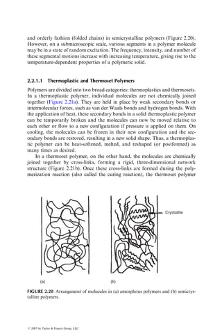
Carbon fibers are commercially available in three basic forms, namely, long
and continuous tow, chopped (6–50 mm long), and milled (30–3000 mm
long). The long and continuous tow, which is simply an untwisted bundle of
1,000–160,000 parallel filaments, is used for high-performance applications.
The price of carbon fiber tow decreases with increasing filament count.
Although high filament counts are desirable for improving productivity in
continuous molding operations, such as filament winding and pultrusion, it
becomes increasingly difficult to wet them with the matrix. ‘‘Dry’’ filaments are
not conducive to good mechanical properties.
Pressure
Spinneret
Orifice
Molten
mesophase
pitch
molecules
Pitch
filament
FIGURE 2.17 Alignment of mesophase pitch into a pitch filament. (After Commercial
Opportunities for Advanced Composites, ASTM STP, 704, 1980.)
ß 2007 by Taylor Francis Group, LLC.](https://image.slidesharecdn.com/fiberreinforcedcompositesmaterialsmanufacturinganddesignp1-220510152925-9ef3de0d/85/Fiber_Reinforced_Composites_Materials_Manufacturing_and_Design_P-1-pdf-71-320.jpg)
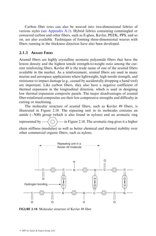
![Kevlar 49 filaments are manufactured by extruding an acidic solution of a
proprietary precursor (a polycondensation product of terephthaloyol chloride
and p-phenylene diamine) from a spinneret. During the filament drawing
process, Kevlar 49 molecules become highly oriented in the direction of the
filament axis. Weak hydrogen bonds between hydrogen and oxygen atoms in
adjacent molecules hold them together in the transverse direction. The resulting
filament is highly anisotropic, with much better physical and mechanical prop-
erties in the longitudinal direction than in the radial direction.
Although the tensile stress–strain behavior of Kevlar 49 is linear, fiber
fracture is usually preceded by longitudinal fragmentation, splintering, and even
localized drawing. In bending, Kevlar 49 fibers exhibit a high degree of yielding on
the compression side. Such a noncatastrophic failure mode is not observed in glass
or carbon fibers, and gives Kevlar 49 composites superior damage tolerance
against impact or other dynamic loading. One interesting application of this
characteristic of Kevlar 49 fibers is found in soft lightweight body armors and
helmets used for protecting police officers and military personnel.
Kevlar 49 fibers do not melt or support combustion but will start to
carbonize at about 4278C. The maximum long-term use temperature recom-
mended for Kevlar 49 is 1608C. They have very low thermal conductivity, but a
very high vibration damping coefficient. Except for a few strong acids and
alkalis, their chemical resistance is good. However, they are quite sensitive to
ultraviolet lights. Prolonged direct exposure to sunlight causes discoloration
and significant loss in tensile strength. The problem is less pronounced in
composite laminates in which the fibers are covered with a matrix. Ultraviolet
light-absorbing fillers can be added to the matrix to further reduce the problem.
Kevlar 49 fibers are hygroscopic and can absorb up to 6% moisture at 100%
relative humidity and 238C. The equilibrium moisture content (i.e., maximum
moisture absorption) is directly proportional to relative humidity and is
attained in 16–36 h. Absorbed moisture seems to have very little effect on the
tensile properties of Kevlar 49 fibers. However, at high moisture content, they
tend to crack internally at the preexisting microvoids and produce longitudinal
splitting [7].
A second-generation Kevlar fiber is Kevlar 149, which has the highest
tensile modulus of all commercially available aramid fibers. The tensile modulus
of Kevlar 149 is 40% higher than that of Kevlar 49; however, its strain-to-failure
is lower. Kevlar 149 has the equilibrium moisture content of 1.2% at 65% relative
humidity and 228C, which is nearly 70% lower than that of Kevlar 49 under
similar conditions. Kevlar 149 also has a lower creep rate than Kevlar 49.
2.1.4 EXTENDED CHAIN POLYETHYLENE FIBERS
Extended chain polyethylene fibers, commercially available under the trade
name Spectra, are produced by gel spinning a high-molecular-weight polyethyl-
ene. Gel spinning yields a highly oriented fibrous structure with exceptionally
ß 2007 by Taylor Francis Group, LLC.](https://image.slidesharecdn.com/fiberreinforcedcompositesmaterialsmanufacturinganddesignp1-220510152925-9ef3de0d/85/Fiber_Reinforced_Composites_Materials_Manufacturing_and_Design_P-1-pdf-73-320.jpg)
![high crystallinity (95%–99%) relative to melt spinning used for conventional
polyethylene fibers.
Spectra polyethylene fibers have the highest strength-to-weight ratio of all
commercial fibers available to date. Two other outstanding features of Spectra
fibers are their low moisture absorption (1% compared with 5%–6% for Kevlar
49) and high abrasion resistance, which make them very useful in marine
composites, such as boat hulls and water skis.
The melting point of Spectra fibers is 1478C; however, since they exhibit a
high level of creep above 1008C, their application temperature is limited to
808C–908C. The safe manufacturing temperature for composites containing Spec-
tra fibers is below 1258C, since they exhibit a significant and rapid reduction in
strength as well as increase in thermal shrinkage above this temperature. Another
problemwithSpectrafibersistheirpooradhesionwithresinmatrices,whichcanbe
partially improved by their surface modification with gas plasma treatment.
Spectra fibers provide high impact resistance for composite laminates even
at low temperatures and are finding growing applications in ballistic composites,
such as armors, helmets, and so on. However, their use in high-performance
aerospace composites is limited, unless they are used in conjunction with stiffer
carbon fibers to produce hybrid laminates with improved impact damage
tolerance than all-carbon fiber laminates.
2.1.5 NATURAL FIBERS
Examples of natural fibers are jute, flax, hemp, remi, sisal, coconut fiber (coir),
and banana fiber (abaca). All these fibers are grown as agricultural plants in
various parts of the world and are commonly used for making ropes, carpet
backing, bags, and so on. The components of natural fibers are cellulose
microfibrils dispersed in an amorphous matrix of lignin and hemicellulose [8].
Depending on the type of the natural fiber, the cellulose content is in the range
of 60–80 wt% and the lignin content is in the range of 5–20 wt%. In addition,
the moisture content in natural fibers can be up to 20 wt%. The properties of
some of the natural fibers in use are given in Table 2.5.
TABLE 2.5
Properties of Selected Natural Fibers
Property Hemp Flax Sisal Jute
Density (g=cm3
) 1.48 1.4 1.33 1.46
Modulus (GPa) 70 60–80 38 10–30
Tensile strength (MPa) 550–900 800–1500 600–700 400–800
Elongation to failure (%) 1.6 1.2–1.6 2–3 1.8
Source: Adapted from Wambua, P., Ivens, J., and Verpoest, I., Compos. Sci. Tech., 63, 1259, 2003.
ß 2007 by Taylor Francis Group, LLC.](https://image.slidesharecdn.com/fiberreinforcedcompositesmaterialsmanufacturinganddesignp1-220510152925-9ef3de0d/85/Fiber_Reinforced_Composites_Materials_Manufacturing_and_Design_P-1-pdf-74-320.jpg)
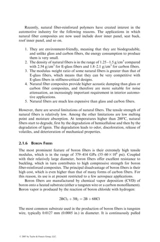
![through a reaction chamber in which boron is deposited on its surface at
11008C–13008C. The speed of pulling and the deposition temperature can be
varied to control the resulting fiber diameter. Currently, commercial boron
fibers are produced in diameters of 0.1, 0.142, and 0.203 mm (0.004, 0.0056, and
0.008 in.), which are much larger than those of other reinforcing fibers.
During boron deposition, the tungsten substrate is converted into tungsten
boride by diffusion and reaction of boron with tungsten. The core diameter
increases in diameter from 0.0127 mm (0.0005 in.) to 0.0165 mm (0.00065 in.),
placing boron near the core in tension. However, near the outer surface of the
boron layer, a state of biaxial compression exists, which makes the boron fiber
less sensitive to mechanical damage [9]. The adverse reactivity of boron fibers
with metals is reduced by chemical vapor deposition of silicon carbide on boron
fibers, which produces borsic fibers.
2.1.7 CERAMIC FIBERS
Silicon carbide (SiC) and aluminum oxide (Al2O3) fibers are examples of
ceramic fibers notable for their high-temperature applications in metal and
ceramic matrix composites. Their melting points are 28308C and 20458C,
respectively. Silicon carbide retains its strength well above 6508C, and alumi-
num oxide has excellent strength retention up to about 13708C. Both fibers are
suitable for reinforcing metal matrices in which carbon and boron fibers exhibit
adverse reactivity. Aluminum oxide fibers have lower thermal and electrical
conductivities and have higher coefficient of thermal expansion than silicon
carbide fibers.
Silicon carbide fibers are available in three different forms [10]:
1. Monofilaments that are produced by chemical vapor deposition of b-SiC
on a 10–25 mm diameter carbon monofilament substrate. The carbon
monofilament is previously coated with ~1 mm thick pyrolitic graphite to
smoothen its surface as well as to enhance its thermal conductivity. b-SiC
is produced by the reaction of silanes and hydrogen gases at around
13008C. The average fiber diameter is 140 mm.
2. Multifilament yarn produced by melt spinning of a polymeric precursor,
such as polycarbosilane, at 3508C in nitrogen gas. The resulting poly-
carbosilane fiber is first heated in air to 1908C for 30 min to cross-link
the polycarbosilane molecules by oxygen and then heat-treated to
10008C–12008C to form a crystalline structure. The average fiber dia-
meter in the yarn is 14.5 mm and a commercial yarn contains 500 fibers.
Yarn fibers have a considerably lower strength than the monofilaments.
3. Whiskers, which are 0.1–1 mm in diameter and around 50 mm in length.
They are produced from rice hulls, which contain 10–20 wt% SiO2. Rice
hulls are first heated in an oxygen-free atmosphere to 7008C–9008C to
remove the volatiles and then to 15008C–16008C for 1 h to produce SiC
ß 2007 by Taylor Francis Group, LLC.](https://image.slidesharecdn.com/fiberreinforcedcompositesmaterialsmanufacturinganddesignp1-220510152925-9ef3de0d/85/Fiber_Reinforced_Composites_Materials_Manufacturing_and_Design_P-1-pdf-76-320.jpg)
![whiskers. The final heat treatment is at 8008C in air, which removes free
carbon. The resulting SiC whiskers contain 10 wt% of SiO2 and up to 10
wt% Si3N4. The tensile modulus and tensile strength of these whiskers
are reported as 700 GPa and 13 GPa (101.5 3 106
psi and 1.88 3 106
psi),
respectively.
Many different aluminum oxide fibers have been developed over the years, but
many of them at present are not commercially available. One of the early
aluminum oxide fibers, but not currently available in the market, is called the
Fiber FP [11]. It is a high-purity (99%) polycrystalline a-Al2O3 fiber, dry spun
from a slurry mix of alumina and proprietary spinning additives. The spun
filaments are fired in two stages: low firing to control shrinkage, followed by
flame firing to produce a suitably dense a-Al2O3. The fired filaments may be
coated with a thin layer of silica to improve their strength (by healing the
surface flaws) as well as their wettability with the matrix. The filament diameter
is 20 mm. The tensile modulus and tensile strength of Fiber FP are reported as
379 GPa and 1.9 GPa (55 3 106
psi and 275,500 psi), respectively. Experiments
have shown that Fiber FP retains almost 100% of its room temperature tensile
strength after 300 h of exposure in air at 10008C. Borsic fiber, on the other
hand, loses 50% of its room temperature tensile strength after only 1 h of
exposure in air at 5008C. Another attribute of Fiber FP is its remarkably high
compressive strength, which is estimated to be about 6.9 GPa (1,000,000 psi).
Nextel 610 and Nextel 720, produced by 3 M, are two of the few aluminum
oxide fibers available in the market now [12]. Both fibers are produced in
continuous multifilament form using the sol–gel process. Nextel 610 contains
greater than 99% Al2O3 and has a single-phase structure of a-Al2O3. The
average grain size is 0.1 mm and the average filament diameter is 14 mm.
Because of its fine-grained structure, it has a high tensile strength at room
temperature; but because of grain growth, its tensile strength decreases rapidly
as the temperature is increased above 11008C. Nextel 720, which contains 85%
Al2O3 and 15% SiO2, has a lower tensile strength at room temperature, but is
able to retain about 85% of its tensile strength even at 14008C. Nextel 720 also
has a much lower creep rate than Nextel 610 and other oxide fibers at temper-
atures above 10008C. The structure of Nextel 720 contains a-Al2O3 grains
embedded in mullite grains. The strength retention of Nextel 720 at high
temperatures is attributed to reduced grain boundary sliding and reduced
grain growth.
Another ceramic fiber, containing approximately equal parts of Al2O3 and
silica (SiO2), is available in short, discontinuous lengths under the trade name
Fiberfrax. The fiber diameter is 2–12 mm and the fiber aspect ratio (length to
diameter ratio) is greater than 200. It is manufactured either by a melt blowing
or by a melt spinning process. Saffil, produced by Saffil Ltd., is also a discon-
tinuous aluminosilicate fiber, containing 95% Al2O3 and 5% SiO2. Its diameter
is 1–5 mm. It is produced by blow extrusion of partially hydrolyzed solution of
ß 2007 by Taylor Francis Group, LLC.](https://image.slidesharecdn.com/fiberreinforcedcompositesmaterialsmanufacturinganddesignp1-220510152925-9ef3de0d/85/Fiber_Reinforced_Composites_Materials_Manufacturing_and_Design_P-1-pdf-77-320.jpg)

![(0.01 in.) from its initial room temperature deflection is called the HDT at the
specific fiber stress.
Although HDT is widely reported in the plastics product literature, it
should not be used in predicting the elevated temperature performance of a
polymer. It is used mostly for quality control and material development pur-
poses. It should be pointed out that HDT is not a measure of the glass
transition temperature. For glass transition temperature measurements, such
methods as differential scanning calorimetry (DSC) or differential thermal
analysis (DTA) are used [13].
2.2.1.5 Selection of Matrix: Thermosets vs. Thermoplastics
The primary consideration in the selection of a matrix is its basic mechanical
properties. For high-performance composites, the most desirable mechanical
properties of a matrix are
1. High tensile modulus, which influences the compressive strength of the
composite
2. High tensile strength, which controls the intraply cracking in a compos-
ite laminate
3. High fracture toughness, which controls ply delamination and crack
growth
For a polymer matrix composite, there may be other considerations, such as
good dimensional stability at elevated temperatures and resistance to moisture
or solvents. The former usually means that the polymer must have a high glass
transition temperature Tg. In practice, the glass transition temperature should
be higher than the maximum use temperature. Resistance to moisture and
solvent means that the polymer should not dissolve, swell, crack (craze), or
otherwise degrade in hot–wet environments or when exposed to solvents. Some
common solvents in aircraft applications are jet fuels, deicing fluids, and paint
strippers. Similarly, gasoline, motor oil, and antifreeze are common solvents in
the automotive environment.
Traditionally, thermoset polymers (also called resins) have been used as a
matrix material for fiber-reinforced composites. The starting materials used in
the polymerization of a thermoset polymer are usually low-molecular-weight
liquid chemicals with very low viscosities. Fibers are either pulled through or
immersed in these chemicals before the polymerization reaction begins. Since
the viscosity of the polymer at the time of fiber incorporation is very low, it is
possible to achieve a good wet-out between the fibers and the matrix without
the aid of either high temperature or pressure. Fiber surface wetting is
extremely important in achieving fiber–matrix interaction in the composite,
an essential requirement for good mechanical performance. Among other
ß 2007 by Taylor Francis Group, LLC.](https://image.slidesharecdn.com/fiberreinforcedcompositesmaterialsmanufacturinganddesignp1-220510152925-9ef3de0d/85/Fiber_Reinforced_Composites_Materials_Manufacturing_and_Design_P-1-pdf-85-320.jpg)
![4. Ease of joining and repair by welding, solvent bonding, and so on
5. Ease of handling (no tackiness)
6. Can be reprocessed and recycled
In spite of such distinct advantages, the development of continuous fiber-
reinforced thermoplastic matrix composites has been much slower than that
of continuous fiber-reinforced thermoset matrix composites. Because of their
high melt or solution viscosities, incorporation of continuous fibers into a
thermoplastic matrix is difficult. Commercial engineering thermoplastic poly-
mers, such as nylons and polycarbonate, are of very limited interest in struc-
tural applications because they exhibit lower creep resistance and lower thermal
stability than thermoset polymers. Recently, a number of thermoplastic poly-
mers have been developed that possess high heat resistance (Table 2.7) and they
are of interest in aerospace applications.
2.2.2 METAL MATRIX
Metal matrix has the advantage over polymeric matrix in applications requiring
a long-term resistance to severe environments, such as high temperature [14].
The yield strength and modulus of most metals are higher than those for
polymers, and this is an important consideration for applications requiring
high transverse strength and modulus as well as compressive strength for the
composite. Another advantage of using metals is that they can be plastically
deformed and strengthened by a variety of thermal and mechanical treatments.
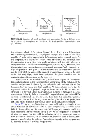
However, metals have a number of disadvantages, namely, they have high
TABLE 2.7
Maximum Service Temperature for Selected Polymeric Matrices
Polymer Tg, 8C Maximum Service Temperature, 8C (8F)
Thermoset matrix
DGEBA epoxy 180 125 (257)
TGDDM epoxy 240–260 190 (374)
Bismaleimides (BMI) 230–290 232 (450)
Acetylene-terminated polyimide (ACTP) 320 280 (536)
PMR-15 340 316 (600)
Thermoplastic matrix
Polyether ether ketone (PEEK) 143 250 (482)
Polyphenylene sulfide (PPS) 85 240 (464)
Polysulfone 185 160 (320)
Polyetherimide (PEI) 217 267 (512)
Polyamide-imide (PAI) 280 230 (446)
K-III polyimide 250 225 (437)
LARC-TPI polyimide 265 300 (572)
ß 2007 by Taylor Francis Group, LLC.](https://image.slidesharecdn.com/fiberreinforcedcompositesmaterialsmanufacturinganddesignp1-220510152925-9ef3de0d/85/Fiber_Reinforced_Composites_Materials_Manufacturing_and_Design_P-1-pdf-87-320.jpg)
![densities, high melting points (therefore, high process temperatures), and a
tendency toward corrosion at the fiber–matrix interface.
The two most commonly used metal matrices are based on aluminum and
titanium. Both of these metals have comparatively low densities and are avail-
able in a variety of alloy forms. Although magnesium is even lighter, its great
affinity toward oxygen promotes atmospheric corrosion and makes it less
suitable for many applications. Beryllium is the lightest of all structural metals
and has a tensile modulus higher than that of steel. However, it suffers from
extreme brittleness, which is the reason for its exclusion as a potential matrix
material. Nickel- and cobalt-based superalloys have also been used as matrix;
however, the alloying elements in these materials tend to accentuate the oxida-
tion of fibers at elevated temperatures.
Aluminum and its alloys have attracted the most attention as matrix
material in metal matrix composites. Commercially, pure aluminum has been
used for its good corrosion resistance. Aluminum alloys, such as 201, 6061, and
1100, have been used for their higher tensile strength–weight ratios. Carbon
fiber is used with aluminum alloys; however, at typical fabrication temperatures
of 5008C or higher, carbon reacts with aluminum to form aluminum carbide
(Al4C3), which severely degrades the mechanical properties of the composite.
Protective coatings of either titanium boride (TiB2) or sodium has been used on
carbon fibers to reduce the problem of fiber degradation as well as to improve their
wetting with the aluminum alloy matrix [15]. Carbon fiber-reinforced aluminum
composites are inherently prone to galvanic corrosion, in which carbon fibers
act as a cathode owing to a corrosion potential of 1 V higher than that of
aluminum. A more common reinforcement for aluminum alloys is SiC.
Titanium alloys that are most useful in metal matrix composites [16] are a,
b alloys (e.g., Ti-6Al-9V) and metastable b-alloys (e.g., Ti-10V-2Fe-3Al). These
titanium alloys have higher tensile strength–weight ratios as well as better
strength retentions at 4008C–5008C over those of aluminum alloys. The thermal
expansion coefficient of titanium alloys is closer to that of reinforcing fibers,
which reduces the thermal mismatch between them. One of the problems with
titanium alloys is their high reactivity with boron and Al2O3 fibers at normal
fabrication temperatures. Borsic (boron fibers coated with silicon carbide) and
silicon carbide (SiC) fibers show less reactivity with titanium. Improved
tensile strength retention is obtained by coating boron and SiC fibers with
carbon-rich layers.
2.2.3 CERAMIC MATRIX
Ceramics are known for their high temperature stability, high thermal shock
resistance, high modulus, high hardness, high corrosion resistance, and low
density. However, they are brittle materials and possess low resistance to crack
propagation, which is manifested in their low fracture toughness. The primary
reason for reinforcing a ceramic matrix is to increase its fracture toughness.
ß 2007 by Taylor Francis Group, LLC.](https://image.slidesharecdn.com/fiberreinforcedcompositesmaterialsmanufacturinganddesignp1-220510152925-9ef3de0d/85/Fiber_Reinforced_Composites_Materials_Manufacturing_and_Design_P-1-pdf-88-320.jpg)
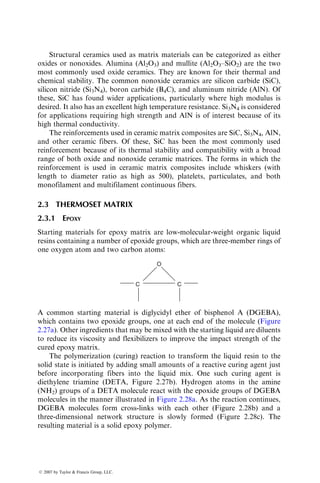
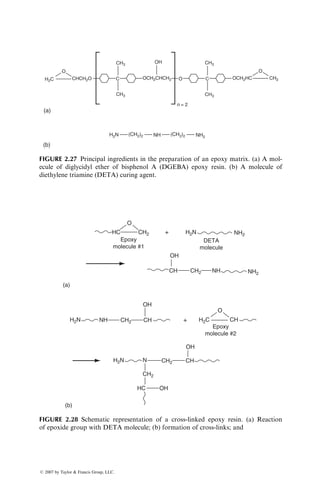
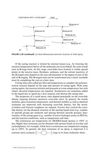
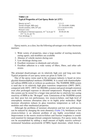
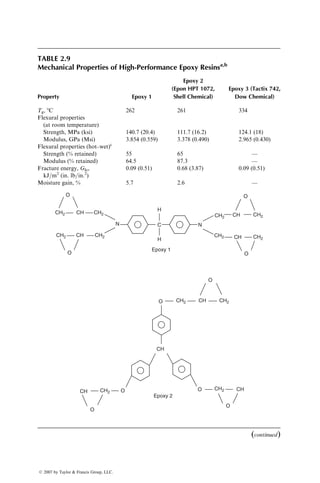
![second phase in the cured matrix and impedes its microcracking. Although the
resin is toughened, its glass transition temperature, modulus, and tensile
strength as well as solvent resistance are reduced (Table 2.10). This problem
is overcome by blending epoxy with a tough thermoplastic resin, such as
polyethersulfone, but the toughness improvement depends on properly match-
ing the epoxy and thermoplastic resin functionalities, their molecular weights,
and so on [17].
2.3.2 POLYESTER
The starting material for a thermoset polyester matrix is an unsaturated poly-
ester resin that contains a number of C¼
¼C double bonds. It is prepared by the
TABLE 2.9 (continued)
Mechanical Properties of High-Performance Epoxy Resinsa,b
Epoxy 3
CH2
CH2
CH3
CH3
CH3 CH3 CH2 CH2
CH
CH2
CH
CH2
CH3
CH3
CH3
CH3
CH2
CH
CH2 CH
N C
O
C N
O
O
O
a
All epoxies were cured with DDS.
b
Molecular structures for Epoxies 1–3 are given in the accompanying figures.
c
Percent retained with room temperature and dry properties when tested in water at 938C after 2
week immersion at 938C.
TABLE 2.10
Effect of CTBN Addition on the Properties of Cast Epoxy Resin
CTBN parts per 100 parts of epoxya
0 5 10 15
Tensile strength, MPa 65.8 62.8 58.4 51.4
Tensile modulus, GPa 2.8 2.5 2.3 2.1
Elongation at break (%) 4.8 4.6 6.2 8.9
Fracture energy, GIc, kJ=m2
1.75 26.3 33.3 47.3
HDT, 8C (at 1.82 MPa) 80 76 74 71
Source: Adapted from Riew, C.K., Rowe, E.H., and Siebert, A.R., Toughness and Brittleness of
Plastics, R.D. Deanin and A.M. Crugnola, eds., American Chemical Society, Washington, D.C.,
1976.
a
DGEBA epoxy (Epon 828, Shell) cured with five parts of piperidine at 1208C for 16 h.
ß 2007 by Taylor Francis Group, LLC.](https://image.slidesharecdn.com/fiberreinforcedcompositesmaterialsmanufacturinganddesignp1-220510152925-9ef3de0d/85/Fiber_Reinforced_Composites_Materials_Manufacturing_and_Design_P-1-pdf-94-320.jpg)
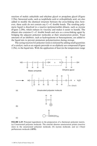
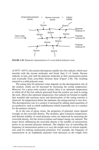
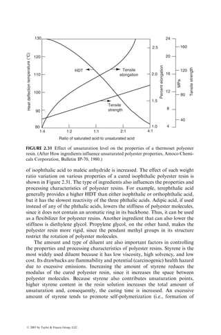
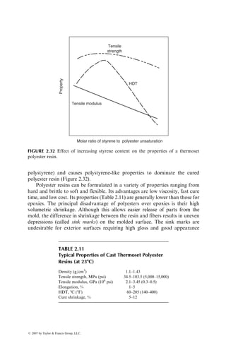
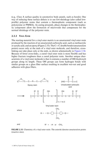
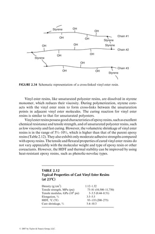
![2.3.4 BISMALEIMIDES AND OTHER THERMOSET POLYIMIDES
Bismaleimide (BMI), PMR-15 (for polymerization of monomer reactants), and
acetylene-terminated polyimide (ACTP) are examples of thermoset polyimides
(Table 2.13). Among these, BMIs are suitable for applications requiring a
service temperature of 1278C–2328C. PMR and ACTP can be used up to
2888C and 3168C, respectively. PMR and ACTP also have exceptional
thermo-oxidative stability and show only 20% weight loss over a period of
1000 h at 3168C in flowing air [18].
Thermoset polyimides are obtained by addition polymerization of liquid
monomeric or oligomeric imides to form a cross-linked infusible structure.
They are available either in solution form or in hot-melt liquid form. Fibers
can be coated with the liquid imides or their solutions before the cross-linking
reaction. On curing, they not only offer high temperature resistance, but also
high chemical and solvent resistance. However, these materials are inherently
very brittle due to their densely cross-linked molecular structure. As a result,
their composites are prone to excessive microcracking. One useful method of
reducing their brittleness without affecting their heat resistance is to combine
them with one or more tough thermoplastic polyimides. The combination
produces a semi-interpenetrating network (semi-IPN) polymer [19], which
retains the easy processability of a thermoset and exhibits the good toughness
of a thermoplastic. Although the reaction time is increased, this helps in
broadening the processing window, which otherwise is very narrow for some
TABLE 2.13
Properties of Thermoset Polyimide Resins (at 238C)
Bismaleimidea
Property
Without
Modifier
Withb
Modifier PMR-15c
ACTPd
Density (g=cm3
) — 1.28 1.32 1.34
Tensile strength, MPa (ksi) — — 38.6 (5.6) 82.7 (12)
Tensile modulus, GPa (Msi) — — 3.9 (0.57) 4.1 (0.60)
Strain-to-failure (%) — — 1.5 1.5
Flexural strength, MPa (ksi) 60 (8.7) 126.2 (18.3) 176 (25.5) 145 (21)
Flexural modulus, GPa (Msi) 5.5 (0.8) 3.7 (0.54) 4 (0.58) 4.5 (0.66)
Fracture energy, GIc,
J=m2
(in. lb=in.2
)
24.5 (0.14) 348 (1.99) 275 (1.57) —
a
Compimide 353 (Shell Chemical Co.).
b
Compimide 353 melt blended with a bis-allylphenyl compound (TM 121), which acts as a
toughening modifier (Shell Chemical Co.).
c
From Ref. [18].
d
Thermid 600 (National Starch and Chemical Corporation).
ß 2007 by Taylor Francis Group, LLC.](https://image.slidesharecdn.com/fiberreinforcedcompositesmaterialsmanufacturinganddesignp1-220510152925-9ef3de0d/85/Fiber_Reinforced_Composites_Materials_Manufacturing_and_Design_P-1-pdf-101-320.jpg)
![of these polyimides and causes problems in manufacturing large or complex
composite parts.
BMIs are the most widely used thermoset polyimides in the advanced
composite industry. BMI monomers (prepolymers) are prepared by the reac-
tion of maleic anhydride with a diamine. A variety of BMI monomers can be
prepared by changing the diamine. One commercially available BMI monomer
has the following chemical formula:
N C N
H
H
Bismaleimide (BMI)
C
C
C
C
O
O
C
C
C
C
O
O
BMI monomers are mixed with reactive diluents to reduce their viscosity and
other comonomers, such as vinyl, acrylic, and epoxy, to improve the toughness
of cured BMI. The handling and processing techniques for BMI resins are
similar to those for epoxy resins. The curing of BMI occurs through addition-
type homopolymerization or copolymerization that can be thermally induced
at 1708C–1908C.
2.3.5 CYANATE ESTER
Cyanate ester resin has a high glass transition temperature (Tg ¼ 2658C), lower
moisture absorption than epoxies, good chemical resistance, and good dimen-
sional stability [20]. Its mechanical properties are similar to those of epoxies.
The curing reaction of cyanate ester involves the formation of thermally stable
triazine rings, which is the reason for its high temperature resistance. The
curing shrinkage of cyanate ester is also relatively small. For all these reasons,
cyanate ester is considered a good replacement for epoxy in some aerospace
applications. Cyanate ester is also considered for printed circuit boards, encap-
sulants, and other electronic components because of its low dielectric constant
and high dielectric breakdown strength, two very important characteristics for
many electronic applications.
Cyanate ester is commonly used in blended form with other polymers. For
example, it is sometimes blended with epoxy to reduce cost. Blending it with
BMI has shown to improve its Tg. Like many other thermoset polymers,
cyanate ester has low fracture toughness. Blending it with thermoplastics,
such as polyarylsulfone and polyethersulfone, has shown to improve its
fracture toughness.
ß 2007 by Taylor Francis Group, LLC.](https://image.slidesharecdn.com/fiberreinforcedcompositesmaterialsmanufacturinganddesignp1-220510152925-9ef3de0d/85/Fiber_Reinforced_Composites_Materials_Manufacturing_and_Design_P-1-pdf-102-320.jpg)
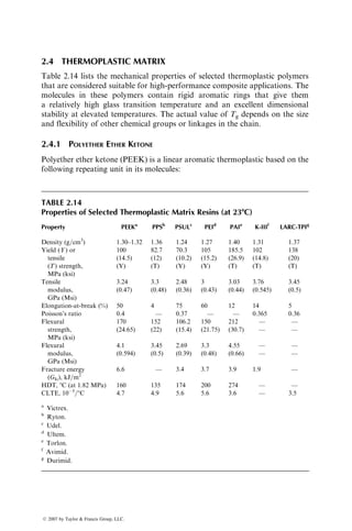
![O
C
Ketone Ether
Polyetherether ketone (PEEK)
Ether
O O
n
Continuous carbon fiber-reinforced PEEK composites are known in the indus-
try as aromatic polymer composite or APC.
PEEK is a semicrystalline polymer with a maximum achievable crystallinity
of 48% when it is cooled slowly from its melt. Amorphous PEEK is produced if
the melt is quenched. At normal cooling rates, the crystallinity is between 30%
and 35%. The presence of fibers in PEEK composites tends to increase the
crystallinity to a higher level, since the fibers act as nucleation sites for crystal
formation [21]. Increasing the crystallinity increases both modulus and yield
strength of PEEK, but reduces its strain-to-failure (Figure 2.35).
PEEK has a glass transition temperature of 1438C and a crystalline melting
point of 3358C. Melt processing of PEEK requires a temperature range of
3708C–4008C. The maximum continuous use temperature is 2508C.
The outstanding property of PEEK is its high fracture toughness, which is
50–100 times higher than that of epoxies. Another important advantage of
PEEK is its low water absorption, which is less than 0.5% at 238C compared
with 4%–5% for conventional aerospace epoxies. As it is semicrystalline, it does
not dissolve in common solvents. However, it may absorb some of these
Stress
(ksi)
Stress
(MPa)
Crystallinity in %
15
12
9
6
3
0 0.2
0.1 0.3 0.4 0.5
0 0
20
40
60
80
100
30%
19%
26%
9%
FIGURE 2.35 Tensile stress–strain diagram of PEEK at different crystallinities.
(Adapted from Seferis, J.C., Polym. Compos., 71, 58, 1986.)
ß 2007 by Taylor Francis Group, LLC.](https://image.slidesharecdn.com/fiberreinforcedcompositesmaterialsmanufacturinganddesignp1-220510152925-9ef3de0d/85/Fiber_Reinforced_Composites_Materials_Manufacturing_and_Design_P-1-pdf-104-320.jpg)
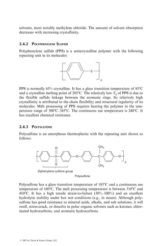
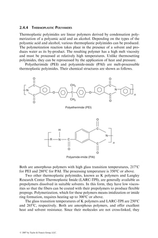
![are not as brittle as thermoset polymers. They are processed with fibers from
low-viscosity solutions much like the thermoset resins; yet after imidization,
they can be made to flow and be shape-formed like conventional thermoplastics
by heating them over their Tg. This latter characteristic is due to the presence of
flexible chemical groups between the stiff, fused-ring imide groups in their
backbones. In LARC-TPI, for example, the sources of flexibility are the carbonyl
groups and the meta-substitution of the phenyl rings in the diamine-derived
portion of the chain. The meta-substitution, in contrast to para-substitution,
allows the polymer molecules to bend and flow.
O
O
LARC-TPI
C
O
C
O
C
C
O
O
C
n
C
N N
2.5 FIBER SURFACE TREATMENTS
The primary function of a fiber surface treatment is to improve the fiber surface
wettability with the matrix and to create a strong bond at the fiber–matrix
interface. Both are essential for effective stress transfer from the matrix to the
fiber and vice versa. Surface treatments for glass, carbon, and Kevlar fibers for
their use in polymeric matrices are described in this section.*
2.5.1 GLASS FIBERS
Chemical coupling agents are used with glass fibers to (1) improve the fiber–
matrix interfacial strength through physical and chemical bonds and (2) protect
the fiber surface from moisture and reactive fluids.
* Several investigators [27] have suggested that there is a thin but distinct interphase between the
fibers and the matrix. The interphase surrounds the fiber and has properties that are different from
the bulk of the matrix. It may be created by local variation of the matrix microstructure close to the
fiber surface. For example, there may be a variation in cross-link density in the case of a thermo-
setting matrix, or a variation of crystallinity in the case of a semicrystalline thermoplastic matrix,
both of which are influenced by the presence of fibers as well as the fiber surface chemistry. The
interphase may also contain microvoids (resulting from poor fiber surface wetting by the matrix or
air entrapment) and unreacted solvents or curing agents that tend to migrate toward the fiber
surface.
ß 2007 by Taylor Francis Group, LLC.](https://image.slidesharecdn.com/fiberreinforcedcompositesmaterialsmanufacturinganddesignp1-220510152925-9ef3de0d/85/Fiber_Reinforced_Composites_Materials_Manufacturing_and_Design_P-1-pdf-107-320.jpg)
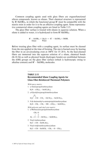
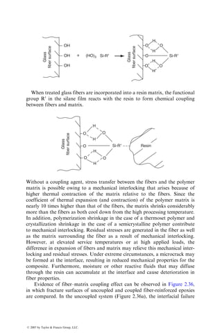
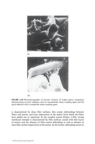
![the fiber–matrix interface, but in the latter, cohesive failure occurs in the
matrix.
The interfacial bond created by silanes or other coupling agents allows a
better load stress transfer between fibers and matrix, which in turn improves
the tensile strength as well as the interlaminar shear strength of the composite.
However, the extent of strength improvement depends on the compatibility of
the coupling agent with the matrix resin. Furthermore, it has been observed
that although a strong interface produces higher strength, a relatively weaker
interface may contribute to higher energy dissipation through debonding at
the fiber–matrix interface, which may be beneficial for attaining higher fracture
toughness.
The data in Table 2.16 show the improvement in strength achieved by
using different silane coupling agents on the glass fiber surface of a glass fiber–
polyester composite. The wet strength of the composite, measured after boiling in
water for 72 h, is lower than the dry strength; however, by adding the silane
coupling agent and creating a stronger interfacial bond between the fibers and the
matrix, the wet strength is significantly improved.
2.5.2 CARBON FIBERS
Carbon fiber surfaces are chemically inactive and must be treated to form
surface functional groups that promote good chemical bonding with the poly-
mer matrix. Surface treatments also increase the surface area by creating
micropores or surface pits on already porous carbon fiber surface. Increase in
surface area provides a larger number of contact points for fiber–matrix bonding.
Commercial surface treatments for carbon fibers are of two types, oxidative
or nonoxidative [4,5]:
TABLE 2.16
Effect of Silane Coupling Agent on the
Strength of E-Glass Fiber-Reinforced
Polyester Rods
Strength (MPa)
Treatment Dry Weta
No silane 916 240
Vinyl silane 740 285
Glycidyl silane 990 380
Methacryl silane 1100 720
a
After boiling in water at 1008C for 72 h.
ß 2007 by Taylor Francis Group, LLC.](https://image.slidesharecdn.com/fiberreinforcedcompositesmaterialsmanufacturinganddesignp1-220510152925-9ef3de0d/85/Fiber_Reinforced_Composites_Materials_Manufacturing_and_Design_P-1-pdf-111-320.jpg)
![1. Oxidative surface treatments produce acidic functional groups, such as
carboxylic, phenolic, and hydroxylic, on the carbon fiber surface. They
may be carried out either in an oxygen-containing gas (air, oxygen, carbon
dioxide, ozone, etc.) or in a liquid (nitric acid, sodium hypochloride, etc.).
The gas-phase oxidation is conducted at 2508C or above and often in
the presence of a catalyst. Oxidation at very high temperatures causes
excessive pitting on the carbon fiber surface and reduces the fiber
strength.
Nitric acid is the most common liquid used for the liquid-phase
oxidation. The effectiveness of treatment in improving the surface prop-
erties depends on the acid concentration, treatment time, and tempera-
ture, as well as the fiber type.
2. Several nonoxidative surface treatments have been developed for carbon
fibers. In one of these treatments, the carbon fiber surface is coated with
an organic polymer that has functional groups capable of reacting with
the resin matrix. Examples of polymer coatings are styrene–maleic
anhydride copolymers, methyl acrylate–acrylonitrile copolymer, and
polyamides. The preferred method of coating the fiber surface is electro-
polymerization, in which carbon fibers are used as one of the electrodes in
an acidic solution of monomers or monomer mixtures [22]. Improved
results are obtained if the carbon fiber surface is oxidized before the
coating process.
2.5.3 KEVLAR FIBERS
Similar to carbon fibers, Kevlar 49 fibers also suffer from weak interfacial
adhesion with most matrix resins. Two methods have been successful in
improving the interfacial adhesion of Kevlar 49 with epoxy resin [7]:
1. Filament surface oxidation or plasma etching, which reduces the fiber
tensile strength but tends to improve the off-axis strength of the com-
posite, which depends on better fiber–matrix interfacial strength.
2. Formation of reactive groups, such as amines (NH2), on the fiber
surface. These reactive groups form covalent bonds with the epoxide
groups across the interface.
2.6 FILLERS AND OTHER ADDITIVES
Fillers are added to a polymer matrix for one or more of the following reasons:
1. Reduce cost (since most fillers are much less expensive than the matrix
resin)
2. Increase modulus
ß 2007 by Taylor Francis Group, LLC.](https://image.slidesharecdn.com/fiberreinforcedcompositesmaterialsmanufacturinganddesignp1-220510152925-9ef3de0d/85/Fiber_Reinforced_Composites_Materials_Manufacturing_and_Design_P-1-pdf-112-320.jpg)
![3. Reduce mold shrinkage
4. Control viscosity
5. Produce smoother surface
The most common filler for polyester and vinyl ester resins is calcium carbonate
(CaCO3), which is used to reduce cost as well as mold shrinkage. Examples of
other fillers are clay, mica, and glass microspheres (solid as well as hollow).
Although fillers increase the modulus of an unreinforced matrix, they tend to
reduce its strength and impact resistance. Typical properties obtained with
calcium carbonate-filled polyester matrix are shown in Table 2.17.
Impact strength and crack resistance of brittle thermosetting polymers can
be improved by mixing them with small amounts of a liquid elastomeric tough-
ener, such as carboxyl-terminated polybutadiene acrylonitrile (CTBN) [23]. In
addition to fillers and tougheners, colorants, flame retardants, and ultraviolet
(UV) absorbers may also be added to the matrix resin [24].
2.7 INCORPORATION OF FIBERS INTO MATRIX
Processes for incorporating fibers into a polymer matrix can be divided into
two categories. In one category, fibers and matrix are processed directly into
the finished product or structure. Examples of such processes are filament
winding and pultrusion. In the second category, fibers are incorporated into
the matrix to prepare ready-to-mold sheets that can be stored and later
processed to form laminated structures by autoclave molding or compres-
sion molding. In this section, we briefly describe the processes used in
preparing these ready-to-mold sheets. Knowledge of these processes will be
helpful in understanding the performance of various composite laminates.
Methods for manufacturing composite structures by filament winding, pul-
trusion, autoclave molding, compression molding, and others are described
in Chapter 5.
Ready-to-mold fiber-reinforced polymer sheets are available in two basic
forms, prepregs and sheet-molding compounds.
TABLE 2.17
Properties of Calcium Carbonate-Filled Polyester Resin
Property Unfilled Polyester Polyester Filled with 30 phr CaCO3
Density, g=cm3
1.30 1.48
HDT, 8C (8F) 79 (174) 83 (181)
Flexural strength, MPa (psi) 121 (17,600) 62 (9,000)
Flexural modulus, GPa (106
psi) 4.34 (0.63) 7.1 (1.03)
ß 2007 by Taylor Francis Group, LLC.](https://image.slidesharecdn.com/fiberreinforcedcompositesmaterialsmanufacturinganddesignp1-220510152925-9ef3de0d/85/Fiber_Reinforced_Composites_Materials_Manufacturing_and_Design_P-1-pdf-113-320.jpg)
![2.7.1 PREPREGS
These are thin sheets of fibers impregnated with predetermined amounts of
uniformly distributed polymer matrix. Fibers may be in the form of continuous
rovings, mat, or woven fabric. Epoxy is the primary matrix material in prepreg
sheets, although other thermoset and thermoplastic polymers have also been
used. The width of prepreg sheets may vary from less than 25 mm (1 in.) to
over 457 mm (18 in.). Sheets wider than 457 mm are called broadgoods.
The thickness of a ply cured from prepreg sheets is normally in the range of
0.13–0.25 mm (0.005–0.01 in.). Resin content in commercially available pre-
pregs is between 30% and 45% by weight.
Unidirectional fiber-reinforced epoxy prepregs are manufactured by pulling
a row of uniformly spaced (collimated) fibers through a resin bath containing
catalyzed epoxy resin dissolved in an appropriate solvent (Figure 2.37). The
solvent is used to control the viscosity of the liquid resin. Fibers preimpreg-
nated with liquid resin are then passed through a chamber in which heat is
applied in a controlled manner to advance the curing reaction to the B-stage. At
the end of B-staging, the prepreg sheet is backed up with a release film or waxed
paper and wound around a take-up roll. The backup material is separated from
the prepreg sheet just before it is placed in the mold to manufacture the
composite part. The normal shelf life (storage time before molding) for epoxy
prepregs is 6–8 days at 238C; however, it can be prolonged up to 6 months or
more if stored at 188C.
2.7.2 SHEET-MOLDING COMPOUNDS
Sheet-molding compounds (SMC) are thin sheets of fibers precompounded
with a thermoset resin and are used primarily in compression molding process
[25]. Common thermoset resins for SMC sheets are polyesters and vinyl esters.
The longer cure time for epoxies has limited their use in SMC.
Controlled heating
elements
Resin solution
Fiber
collimator
Metering device
Take-up roll
Back-up material (Release film)
Fiber package
FIGURE 2.37 Schematic of prepreg manufacturing.
ß 2007 by Taylor Francis Group, LLC.](https://image.slidesharecdn.com/fiberreinforcedcompositesmaterialsmanufacturinganddesignp1-220510152925-9ef3de0d/85/Fiber_Reinforced_Composites_Materials_Manufacturing_and_Design_P-1-pdf-114-320.jpg)
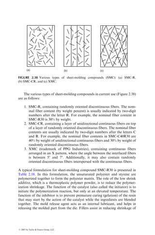
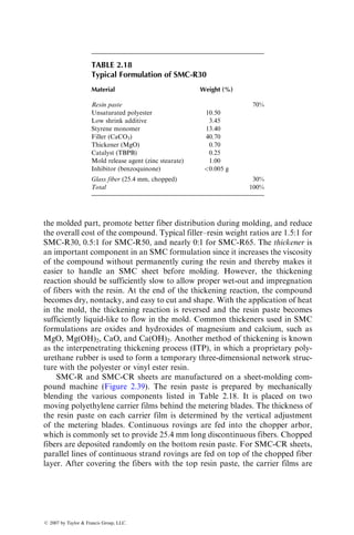
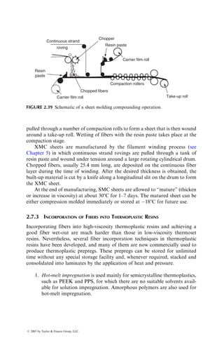
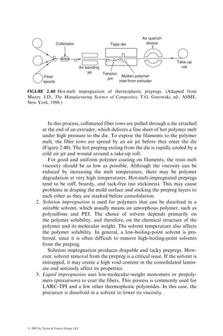
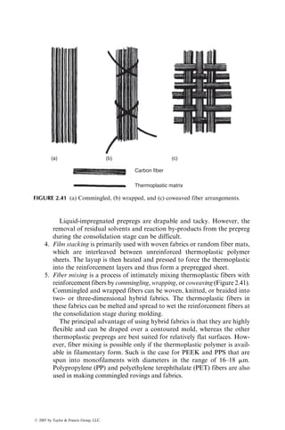
![6. Dry powder coating [26] uses charged and fluidized thermoplastic pow-
ders to coat the reinforcement fibers. After passing through the fluidized
bed, the fibers enter a heated oven, where the polymer coating is melted
on the fiber surface.
2.8 FIBER CONTENT, DENSITY, AND VOID CONTENT
Theoretical calculations for strength, modulus, and other properties of a fiber-
reinforced composite are based on the fiber volume fraction in the material.
Experimentally, it is easier to determine the fiber weight fraction wf, from
which the fiber volume fraction vf and composite density rc can be calculated:
vf ¼
wf=rf
(wf=rf) þ (wm=rm)
, (2:7)
rc ¼
1
(wf=rf) þ (wm=rm)
, (2:8)
where
wf ¼ fiber weight fraction (same as the fiber mass fraction)
wm ¼ matrix weight fraction (same as the matrix mass fraction) and is equal
to (1wf)
rf ¼ fiber density
rm ¼ matrix density
In terms of volume fractions, the composite density rc can be written as
rc ¼ rfvf þ rmvm, (2:9)
where vf is the fiber volume fraction and vm is the matrix volume fraction. Note
that vm is equal to (1vf).
The fiber weight fraction can be experimentally determined by either the
ignition loss method (ASTM D2854) or the matrix digestion method (ASTM
D3171). The ignition loss method is used for PMC-containing fibers that do not
lose weight at high temperatures, such as glass fibers. In this method, the cured
resin is burned off from a small test sample at 5008C–6008C in a muffle furnace.
In the matrix digestion method, the matrix (either polymeric or metallic) is
dissolved away in a suitable liquid medium, such as concentrated nitric acid.
In both cases, the fiber weight fraction is determined by comparing the weights
of the test sample before and after the removal of the matrix. For unidirectional
composites containing electrically conductive fibers (such as carbon) in a
ß 2007 by Taylor Francis Group, LLC.](https://image.slidesharecdn.com/fiberreinforcedcompositesmaterialsmanufacturinganddesignp1-220510152925-9ef3de0d/85/Fiber_Reinforced_Composites_Materials_Manufacturing_and_Design_P-1-pdf-120-320.jpg)

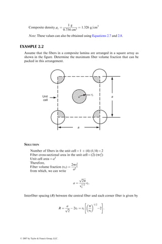
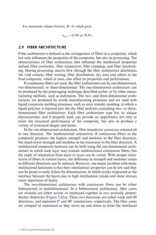
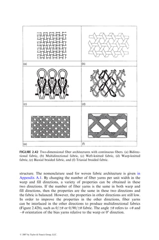

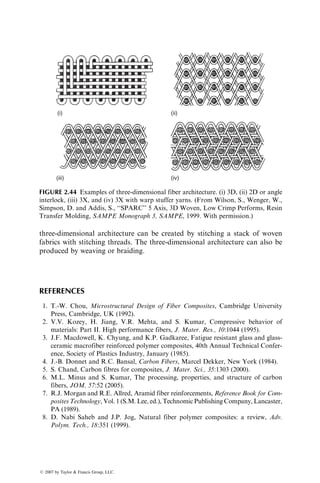
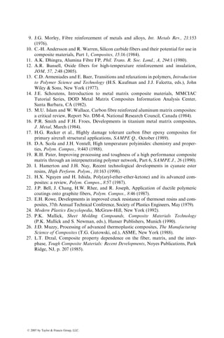
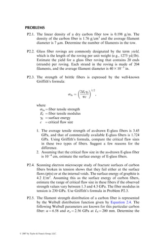
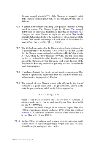
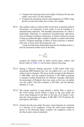

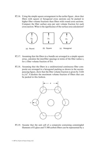
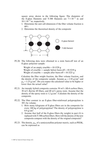
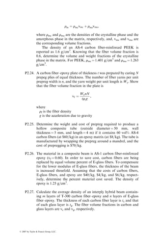

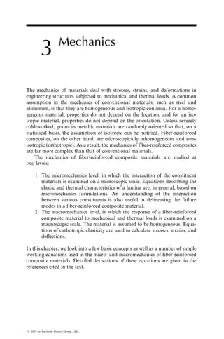
![3.1 FIBER–MATRIX INTERACTIONS IN A UNIDIRECTIONAL
LAMINA
We consider the mechanics of materials approach [1] in describing fiber–matrix
interactions in a unidirectional lamina owing to tensile and compressive load-
ings. The basic assumptions in this vastly simplified approach are as follows:
1. Fibers are uniformly distributed throughout the matrix.
2. Perfect bonding exists between the fibers and the matrix.
3. The matrix is free of voids.
4. The applied force is either parallel to or normal to the fiber direction.
5. The lamina is initially in a stress-free state (i.e., no residual stresses are
present in the fibers and the matrix).
6. Both fibers and matrix behave as linearly elastic materials.
A review of other approaches to the micromechanical behavior of a composite
lamina is given in Ref. [2].
3.1.1 LONGITUDINAL TENSILE LOADING
In this case, the load on the composite lamina is a tensile force applied parallel
to the longitudinal direction of the fibers.
3.1.1.1 Unidirectional Continuous Fibers
Assuming a perfect bonding between fibers and matrix, we can write
«f ¼ «m ¼ «c, (3:1)
where «f, «m, and «c are the longitudinal strains in fibers, matrix, and compos-
ite, respectively (Figure 3.1).
Since both fibers and matrix are elastic, the respective longitudinal stresses
can be calculated as
sf ¼ Ef«f ¼ Ef«c, (3:2)
sm ¼ Em«m ¼ Em«c: (3:3)
Comparing Equation 3.2 with Equation 3.3 and noting that Ef Em, we
conclude that the fiber stress sf is always greater than the matrix stress sm.
The tensile force Pc applied on the composite lamina is shared by the fibers
and the matrix so that
Pc ¼ Pf þ Pm: (3:4)
ß 2007 by Taylor Francis Group, LLC.](https://image.slidesharecdn.com/fiberreinforcedcompositesmaterialsmanufacturinganddesignp1-220510152925-9ef3de0d/85/Fiber_Reinforced_Composites_Materials_Manufacturing_and_Design_P-1-pdf-138-320.jpg)
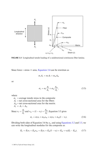
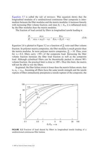
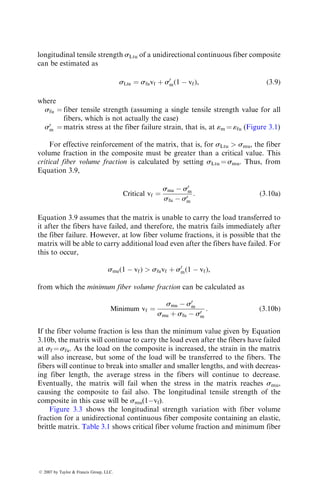
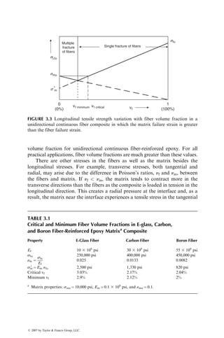
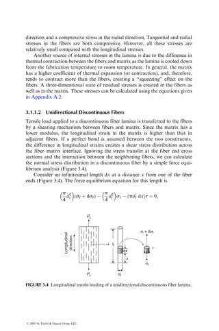
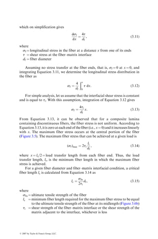

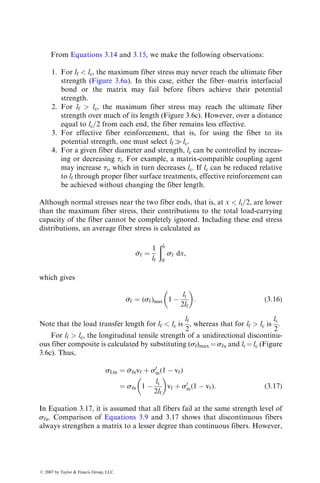
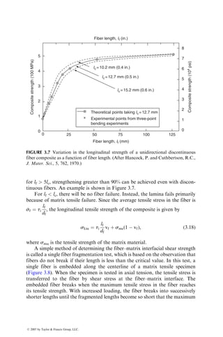
![tensile stress can no longer reach the fiber tensile strength. The fragmented fiber
lengths at this point are theoretically equal to the critical fiber length, lc. How-
ever, actual (measured) fragment lengths vary between lc=2 and lc. Assuming a
uniform distribution for the fragment lengths and a mean value of
l equal to
0.75lc, Equation 3.15 can be used to calculate the interfacial shear strength tim [3]:
tim ¼
3dfsfu
8
l
, (3:19)
where
l is the mean fragment length.
Equation 3.13 was obtained assuming that the interfacial shear stress ti is a
constant. The analysis that followed Equation 3.13 was used to demonstrate
the importance of critical fiber length in discontinuous fiber composites. How-
ever, strictly speaking, this analysis is valid only if it can be shown that ti is a
constant. This will be true in the case of a ductile matrix that yields due to high
shear stress in the interfacial zone before the fiber–matrix bond fails and then
flows plastically with little or no strain hardening (i.e., the matrix behaves as a
perfectly plastic material with a constant yield strength as shown in Figure 3.9).
When this occurs, the interfacial shear stress is equal to the shear yield strength of
the matrix (which is approximately equal to half of its tensile yield strength)
and remains constant at this value. If the fiber–matrix bond fails before matrix
yielding, a frictional force may be generated at the interface, which transfers the
load from the matrix to the fibers through slippage (sliding). In a polymer
matrix composite, the source of this frictional force is the radial pressure on the
fiber surface created by the shrinkage of the matrix as it cools down from the
Fiber embedded
in matrix
Fragmented
fiber
(a)
(b)
FIGURE 3.8 Single fiber fragmentation test to determine fiber–matrix interfacial shear
strength.
ß 2007 by Taylor Francis Group, LLC.](https://image.slidesharecdn.com/fiberreinforcedcompositesmaterialsmanufacturinganddesignp1-220510152925-9ef3de0d/85/Fiber_Reinforced_Composites_Materials_Manufacturing_and_Design_P-1-pdf-148-320.jpg)
![curing temperature. In this case, the interfacial shear stress is equal to the
product of the coefficient of sliding friction and the radial pressure.
When the matrix is in the elastic state and the fiber–matrix bond is still
unbroken, the interfacial shear stress is not a constant and varies with x.
Assuming that the matrix has the same strain as the composite, Cox [4] used
a simple shear lag analysis to derive the following expression for the fiber stress
distribution along the length of a discontinuous fiber:
sf ¼ Ef«1 1
cosh b
lf
2
x
cosh
blf
2
2
6
6
4
3
7
7
5 for 0 x
lf
2
, (3:20)
where
sf ¼ longitudinal fiber stress at a distance x from its end
Ef ¼ fiber modulus
«1 ¼ longitudinal strain in the composite
b ¼
ffiffiffiffiffiffiffiffiffiffiffiffiffiffiffiffiffiffiffiffiffiffiffiffiffiffiffi
2Gm
Efr2
f ln (R=rf)
s
,
where
Gm ¼ matrix shear modulus
rf ¼ fiber radius
2R ¼ center-to-center distance from a fiber to its nearest neighbor
(b) Elastic–strain hardening
(a) Elastic–perfectly plastic
Elastic
modulus
Strain
Stress
smy
FIGURE 3.9 Stress–strain diagrams of (a) an elastic-perfectly plastic material and (b) an
elastic-strain hardening material.
ß 2007 by Taylor Francis Group, LLC.](https://image.slidesharecdn.com/fiberreinforcedcompositesmaterialsmanufacturinganddesignp1-220510152925-9ef3de0d/85/Fiber_Reinforced_Composites_Materials_Manufacturing_and_Design_P-1-pdf-149-320.jpg)
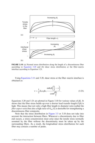
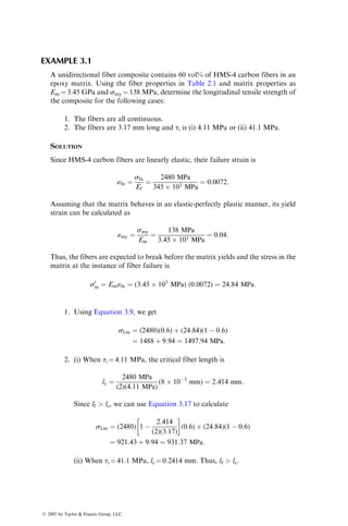
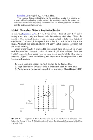
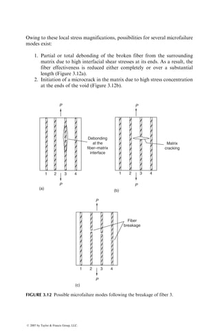
![3. Plastic deformation (microyielding) in the matrix, particularly if the
matrix is ductile.
4. Failure of other fibers in the vicinity of the first fiber break due to high
average normal stresses and the local stress concentrations (Figure
3.12c). Each fiber break creates additional stress concentrations in the
matrix as well as in other fibers. Eventually, many of these fiber breaks
and the surrounding matrix microcracks may join to form a long micro-
crack in the lamina.
The presence of longitudinal stress (syy) concentration at the tip of an advan-
cing crack is well known. Cook and Gordon [5] have shown that the stress
components sxx and txy may also reach high values slightly ahead of the crack
tip (Figure 3.13a). Depending on the fiber–matrix interfacial strength, these
stress components are capable of debonding the fibers from the surrounding
matrix even before they fail in tension (Figure 3.13b). Fiber–matrix debonding
ahead of the crack tip has the effect of blunting the crack front and reducing the
notch sensitivity of the material. High fiber strength and low interfacial
strength promote debonding over fiber tensile failure.
With increasing load, fibers continue to break randomly at various loca-
tions in the lamina. Because of the statistical distribution of surface flaws, the
Debonding
ahead
of the
crack tip
s
syy
sxx
s
x
y
(a) (b)
FIGURE 3.13 Schematic representation of (a) normal stress distributions and (b) fiber–
matrix debonding ahead of a crack tip.
ß 2007 by Taylor Francis Group, LLC.](https://image.slidesharecdn.com/fiberreinforcedcompositesmaterialsmanufacturinganddesignp1-220510152925-9ef3de0d/85/Fiber_Reinforced_Composites_Materials_Manufacturing_and_Design_P-1-pdf-154-320.jpg)
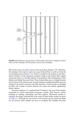
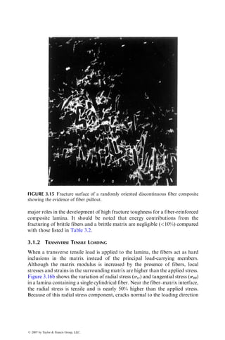
![may develop either at the fiber–matrix interface or in the matrix at u ¼ 908
(Figure 3.16c).
In a lamina containing a high volume fraction of fibers, there will be
interactions of stress fields from neighboring fibers. Adams and Doner [10]
used a finite difference method to calculate the stresses in unidirectional com-
posites under transverse loading. A rectangular packing arrangement of paral-
lel fibers was assumed, and solutions were obtained for various interfiber
spacings representing different fiber volume fractions. Radial stresses at the
fiber–matrix interface for 55% and 75% fiber volume fractions are shown in
Figure 3.17. The maximum principal stress increases with increasing Ef=Em
ratio and fiber volume fraction, as indicated in Figure 3.18. The transverse
modulus of the composite has a similar trend. Although an increased transverse
modulus is desirable in many applications, an increase in local stress concen-
trations at high volume fractions and high fiber modulus may reduce the
transverse strength of the composite (Table 3.3).
The simplest model used for deriving the equation for the transverse modulus
of a unidirectional continuous fiber-reinforced composite is shown in Figure 3.19
TABLE 3.2
Important Energy Absorption Mechanisms During Longitudinal Tensile
Loading of a Unidirectional Continuous Fiber Lamina
Stress relaxation energy (energy dissipated
owing to reduction in stresses at the
ends of a broken fiber [6])
Er ¼
vfs2
fulc
6Ef
Stored elastic energy in a partially
debonded fiber [7]
Es ¼
vfs2
fuy
4Ef
(where y ¼ debonded length of
the fiber when it breaks)
Fiber pullout energy ½8 Epo ¼
vfsful2
c
12lf
for lf lc
¼
vfsful2
f
12lc
for lf lc
Energy absorption by matrix deformation
between parallel matrix cracks [9]
Emd ¼
(1 vf)2
vf
smudf
4ti
Um
(where Um ¼ energy required in deforming
unit volume of the matrix to rupture)
Notes:
1. All energy expressions are on the basis of unit fracture surface area.
2. Debonding of fibers ahead of a crack tip or behind a crack tip is an important energy absorption
mechanism. However, no suitable energy expression is available for this mechanism.
3. Energy absorption may also occur because of yielding of fibers or matrix if either of these
constituents is ductile in nature.
ß 2007 by Taylor Francis Group, LLC.](https://image.slidesharecdn.com/fiberreinforcedcompositesmaterialsmanufacturinganddesignp1-220510152925-9ef3de0d/85/Fiber_Reinforced_Composites_Materials_Manufacturing_and_Design_P-1-pdf-157-320.jpg)
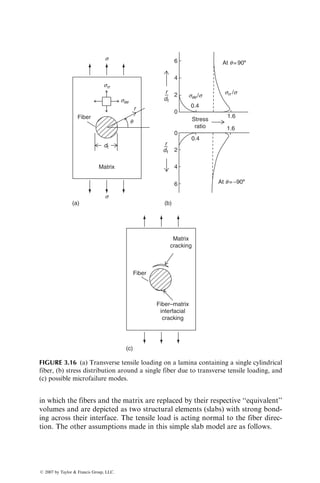
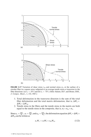
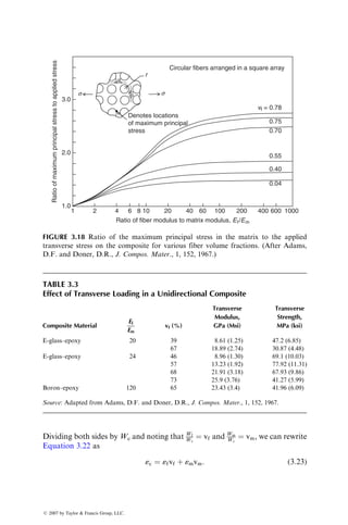
![Since «c ¼
sc
ET
, «f ¼
sf
Ef
, and «m ¼
sm
Em
, Equation 3.23 can be written as
sc
ET
¼
sf
Ef
vf þ
sm
Em
vm: (3:24)
In Equation 3.24, ET is the transverse modulus of the unidirectional continuous
fiber composite.
Finally, since it is assumed that sf ¼ sm ¼ sc, Equation 3.24 becomes
1
ET
¼
vf
Ef
þ
vm
Em
: (3:25)
Rearranging Equation 3.25, the expression for the transverse modulus ET
becomes
ET ¼
EfEm
Efvm þ Emvf
¼
EfEm
Ef vf(Ef Em)
: (3:26)
Equation 3.26 shows that the transverse modulus increases nonlinearly with
increasing fiber volume fraction. By comparing Equations 3.7 and 3.26, it can
be seen that the transverse modulus is lower than the longitudinal modulus and
is influenced more by the matrix modulus than by the fiber modulus.
A simple equation for predicting the transverse tensile strength of a unidir-
ectional continuous fiber lamina [11] is
sTtu ¼
smu
Ks
, (3:27)
Fiber
slab
Matrix
slab
Transverse
direction
Wc
Wf Wm
FIGURE 3.19 Transverse loading of a unidirectional continuous fiber lamina and the
equivalent slab model.
ß 2007 by Taylor Francis Group, LLC.](https://image.slidesharecdn.com/fiberreinforcedcompositesmaterialsmanufacturinganddesignp1-220510152925-9ef3de0d/85/Fiber_Reinforced_Composites_Materials_Manufacturing_and_Design_P-1-pdf-161-320.jpg)
![where
Ks ¼
1 vf[1 (Em=Ef)]
1 (4vf=p)1=2
[1 (Em=Ef)]
:
Equation 3.27 assumes that the transverse tensile strength of the composite is
limited by the ultimate tensile strength of the matrix. Note that Ks represents
the maximum stress concentration in the matrix in which fibers are arranged in
a square array. The transverse tensile strength values predicted by Equation
3.27 are found to be in reasonable agreement with those predicted by the finite
difference method for fiber volume fractions 60% [2]. Equation 3.27 predicts
that for a given matrix, the transverse tensile strength decreases with increasing
fiber modulus as well as increasing fiber volume fraction.
3.1.3 LONGITUDINAL COMPRESSIVE LOADING
An important function of the matrix in a fiber-reinforced composite material is
to provide lateral support and stability for fibers under longitudinal compres-
sive loading. In polymer matrix composites in which the matrix modulus is
relatively low compared with the fiber modulus, failure in longitudinal com-
pression is often initiated by localized buckling of fibers. Depending on whether
the matrix behaves in an elastic manner or shows plastic deformation, two
different localized buckling modes are observed: elastic microbuckling and fiber
kinking.
Rosen [12] considered two possible elastic microbuckling modes of fibers in
an elastic matrix as demonstrated in Figure 3.20. The extensional mode of
(a) (b)
FIGURE 3.20 Fiber microbuckling modes in a unidirectional continuous fiber compos-
ite under longitudinal compressive loading: (a) extensional mode and (b) shear mode.
ß 2007 by Taylor Francis Group, LLC.](https://image.slidesharecdn.com/fiberreinforcedcompositesmaterialsmanufacturinganddesignp1-220510152925-9ef3de0d/85/Fiber_Reinforced_Composites_Materials_Manufacturing_and_Design_P-1-pdf-162-320.jpg)
![microbuckling occurs at low fiber volume fractions (vf 0.2) and creates an
extensional strain in the matrix because of out-of-phase buckling of fibers. The
shear mode of microbuckling occurs at high fiber volume fractions and creates
a shear strain in the matrix because of in-phase buckling of fibers. Using
buckling theory for columns in an elastic foundation, Rosen [12] predicted
the compressive strengths in extensional mode and shear mode as
Extensional mode: sLcu ¼ 2vf
vfEmEf
3(1 vf)
1=2
, (3:28a)
Shear mode: sLcu ¼
Gm
(1 vf)
, (3:28b)
where
Gm is the matrix shear modulus
vf is the fiber volume fraction
Since most fiber-reinforced composites contain fiber volume fraction
30%, the shear mode is more important than the extensional mode. As
Equation 3.28b shows, the shear mode is controlled by the matrix shear
modulus as well as fiber volume fraction. The measured longitudinal compres-
sive strengths are generally found to be lower than the theoretical values
calculated from Equation 3.28b. Some experimental data suggest that the
longitudinal compressive strength follows a rule of mixtures prediction similar
to Equation 3.9.
The second important failure mode in longitudinal compressive loading is
fiber kinking, which occurs in highly localized areas in which the fibers are
initially slightly misaligned from the direction of the compressive loading. Fiber
bundles in these areas rotate or tilt by an additional angle from their initial
configuration to form kink bands and the surrounding matrix undergoes large
shearing deformation (Figure 3.21). Experiments conducted on glass and car-
bon fiber-reinforced composites show the presence of fiber breakage at the ends
of kink bands [13]; however, whether fiber breakage precedes or follows the
kink band formation has not been experimentally verified. Assuming an elastic-
perfectly plastic shear stress–shear strain relationship for the matrix, Budiansky
and Fleck [14] have determined the stress at which kinking is initiated as
sck ¼
tmy
w þ gmy
, (3:29)
where
tmy ¼ shear yield strength of the matrix
gmy ¼ shear yield strain of the matrix
w ¼ initial angle of fiber misalignment
ß 2007 by Taylor Francis Group, LLC.](https://image.slidesharecdn.com/fiberreinforcedcompositesmaterialsmanufacturinganddesignp1-220510152925-9ef3de0d/85/Fiber_Reinforced_Composites_Materials_Manufacturing_and_Design_P-1-pdf-163-320.jpg)
![Besides fiber microbuckling and fiber kinking, a number of other failure modes
have also been observed in longitudinal compressive loading of unidirectional
continuous fiber-reinforced composites. They include shear failure of the com-
posite, compressive failure or yielding of the reinforcement, longitudinal split-
ting in the matrix due to Poisson’s ratio effect, matrix yielding, interfacial
debonding, and fiber splitting or fibrillation (in Kevlar 49 composites). Factors
that appear to improve the longitudinal compressive strength of unidirectional
composites are increasing values of the matrix shear modulus, fiber tensile
modulus, fiber diameter, matrix ultimate strain, and fiber–matrix interfacial
strength. Fiber misalignment or bowing, on the other hand, tends to reduce the
longitudinal compressive strength.
3.1.4 TRANSVERSE COMPRESSIVE LOADING
In transverse compressive loading, the compressive load is applied normal to
the fiber direction, and the most common failure mode observed is the matrix
shear failure along planes that are parallel to the fiber direction, but inclined to
the loading direction (Figure 3.22). The failure is initiated by fiber–matrix
debonding. The transverse compressive modulus and strength are considerably
lower than the longitudinal compressive modulus and strength. The transverse
compressive modulus is higher than the matrix modulus and is close to the
transverse tensile modulus. The transverse compressive strength is found to be
nearly independent of fiber volume fraction [15].
b
a
w
FIGURE 3.21 Kink band geometry. a ¼ Kink band angle, b ¼ Fiber tilt angle, and
v ¼ Kink band width.
ß 2007 by Taylor Francis Group, LLC.](https://image.slidesharecdn.com/fiberreinforcedcompositesmaterialsmanufacturinganddesignp1-220510152925-9ef3de0d/85/Fiber_Reinforced_Composites_Materials_Manufacturing_and_Design_P-1-pdf-164-320.jpg)

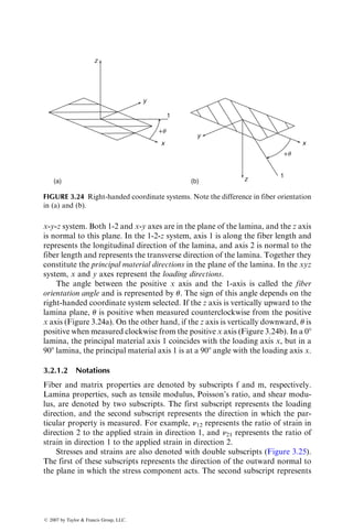
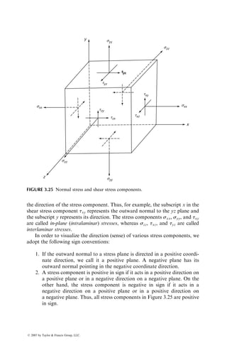
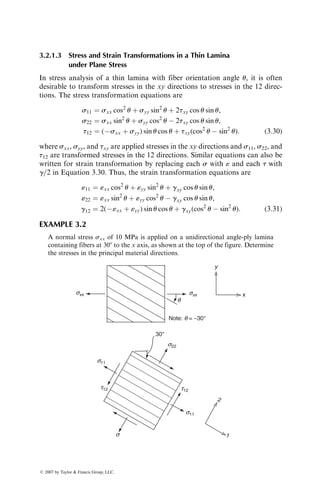
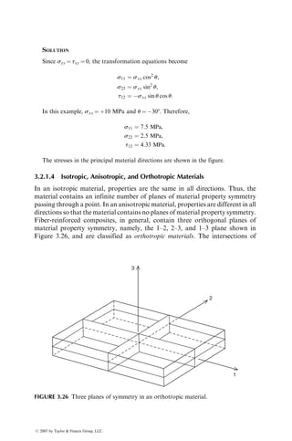
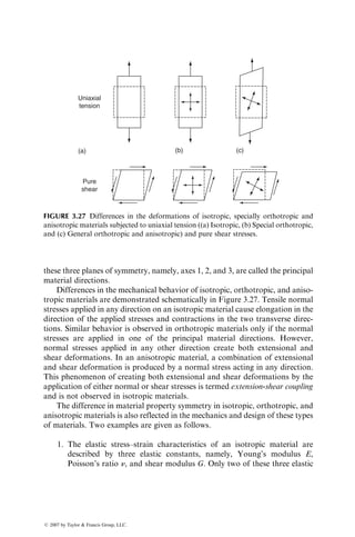
![constants are independent since they can be related by the following
equation:
G ¼
E
2(1 þ n)
: (3:32)
The number of independent elastic constants required to characterize
anisotropic and orthotropic materials are 21 and 9, respectively [16].
For an orthotropic material, the nine independent elastic constants are
E11, E22, E33, G12, G13, G23, n12, n13, and n23.
Unidirectionally oriented fiber composites are a special class
of orthotropic materials. Referring to Figure 3.28, which shows a
Lamina
thickness
1
(Fiber direction)
2
Longitudinal
tension (s11)
Transverse
tension (s22)
Transverse
tension (s33)
In-plane
shear (t12)
Out-of-plane
shear (t23)
Out-of-plane
shear (t13)
3
FIGURE 3.28 Tensile and shear loading on a unidirectional continuous fiber composite.
ß 2007 by Taylor Francis Group, LLC.](https://image.slidesharecdn.com/fiberreinforcedcompositesmaterialsmanufacturinganddesignp1-220510152925-9ef3de0d/85/Fiber_Reinforced_Composites_Materials_Manufacturing_and_Design_P-1-pdf-171-320.jpg)
![composite in which the fibers are in the 12 plane, it can be visualized that
the elastic properties are equal in the 2–3 direction so that E22 ¼ E33,
n12 ¼ n13, and G12 ¼ G13. Furthermore, G23 can be expressed in terms of
E22 and n23 by an expression similar to Equation 3.32.
G23 ¼
E22
2(1 þ n23)
: (3:33)
Thus, the number of independent elastic constants for a unidirectionally
oriented fiber composite reduces to 5, namely, E11, E22, n12, G12, and n23.
Such composites are often called transversely isotropic.
Note that n21 6¼ n12 and n31 6¼ n13, but n31 ¼ n21. However, n21 is
related to n12 by the following equation, and therefore is not an inde-
pendent elastic constant.
n21 ¼
E22
E11
n12: (3:34)
Christensen [17] has shown that in the case of unidirectional fiber-
reinforced composites with fibers oriented in the 1-direction, n23 can
be related to n12 and n21 using the following equation:
n23 ¼ n32 ¼ n12
(1 n21)
(1 n12)
: (3:35)
Equation 3.35 fits the experimental data within the range of experimen-
tal accuracy. Thus, for a unidirectional fiber-reinforced composite, the
number of independent elastic constants is reduced from 5 to 4.
2. For an isotropic material, the sign convention for shear stresses and
shear strains is of little practical significance, since its mechanical behav-
ior is independent of the direction of shear stress. For an orthotropic or
anisotropic material, the direction of shear stress is critically important
in determining its strength and modulus [18]. For example, consider a
unidirectional fiber-reinforced lamina (Figure 3.29) subjected to states
of pure shear of opposite sense. For positive shear (Figure 3.29a), the
maximum (tensile) principal stress is parallel to the fiber direction that
causes fiber fracture. For negative shear (Figure 3.29b), the maximum
(tensile) principal stress is normal to the fiber direction, which causes
either a matrix failure or a fiber–matrix interface failure. Obviously, a
positive shear condition will favor a higher load-carrying capacity than
the negative shear condition. For an isotropic material, shear strength is
equal in all directions. Therefore, the direction of shear stress will not
influence the failure of the material.
ß 2007 by Taylor Francis Group, LLC.](https://image.slidesharecdn.com/fiberreinforcedcompositesmaterialsmanufacturinganddesignp1-220510152925-9ef3de0d/85/Fiber_Reinforced_Composites_Materials_Manufacturing_and_Design_P-1-pdf-172-320.jpg)
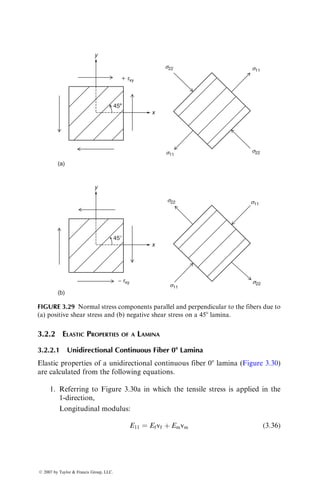
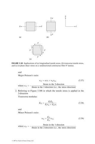
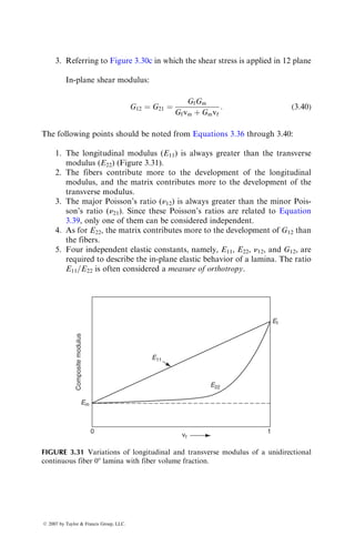
![Equations 3.36 through 3.40 are derived using the simple mechanics of mater-
ials approach along with the following assumptions:
1. Both fibers and matrix are linearly elastic isotropic materials.
2. Fibers are uniformly distributed in the matrix.
3. Fibers are perfectly aligned in the 1-direction.
4. There is perfect bonding between fibers and matrix.
5. The composite lamina is free of voids.
Since, in practice, none of these assumptions is completely valid, these equa-
tions provide only approximate values for the elastic properties of a continuous
fiber 08 lamina. It has been found that the values of E11 and n12 predicted by
Equations 3.36 and 3.37 agree well with the experimental data, but values of
E22 and G12 predicted by Equations 3.38 and 3.40 are lower than the experi-
mental data [19]. Both E22 and G12 are sensitive to void content, fiber anisot-
ropy, and the matrix Poisson’s ratio. Since equations based on the theory of
elasticity or the variational approach, for example, are difficult to solve, Equa-
tions 3.36 through 3.40 or empirically modified versions of these equations (see
Appendix A.3) are used frequently for the laminate design.
In Equations 3.36 through 3.40, it is assumed that both fibers and matrix
are isotropic materials. While the matrix in most fiber-reinforced compo-
sites exhibits isotropic behavior, many reinforcing fibers are not isotropic
and their elastic modulus in the longitudinal direction, EfL, is much greater than
their elastic modulus in the transverse direction, EfT. Accordingly, Equations
3.36 and 3.38 should be modified in the following manner.
E11 ¼ EfLvf þ Emvm, (3:41)
E22 ¼
EfTEm
EfTvm þ Emvf
: (3:42)
The Poisson’s ratio of the fiber in Equation 3.37 should be represented by nfLT,
and its shear modulus in Equation 3.40 should be represented by GfLT. Since for
most of the fibers, EfT, nfLT, and GfLT are difficult to measure and are not
available, Equations 3.36 and 3.40 are commonly used albeit the errors that
they can introduce.
EXAMPLE 3.3
To demonstrate the difference between n12 and n21, consider the following
example in which a square composite plate containing unidirectional continuous
T-300 carbon fiber-reinforced epoxy is subjected to a uniaxial tensile load of 1000 N.
The plate thickness is 1 mm. The length (Lo) and width (Wo) of the plate are
100 mm each.
ß 2007 by Taylor Francis Group, LLC.](https://image.slidesharecdn.com/fiberreinforcedcompositesmaterialsmanufacturinganddesignp1-220510152925-9ef3de0d/85/Fiber_Reinforced_Composites_Materials_Manufacturing_and_Design_P-1-pdf-176-320.jpg)
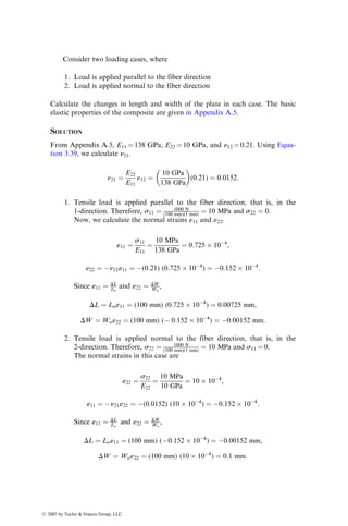
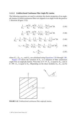
![either greater than E11 or less than E22 at some intermediate values of u. The
range of G12 for which Exx is within E11 and E22 [20] is given by
E11
2(1 þ n12)
G12
E11
2 E11
E22
þ n12
: (3:48)
For glass fiber–epoxy, high-strength carbon fiber–epoxy, and Kevlar 49 fiber–
epoxy composites, G12 is within the range given by Equation 3.48, and therefore,
for these composite laminas, E22 Exx E11. However, for very high-modulus
carbon fiber–epoxy and boron fiber–epoxy composites, G12 is less than the
lower limit in Equation 3.48, and therefore for a range of angles between 08 and
908, Exx for these laminas can be lower than E22.
3.2.2.3 Unidirectional Discontinuous Fiber 08 Lamina
Elastic properties of a unidirectional discontinuous fiber 08 lamina are calcu-
lated using the following equations (Figure 3.34).
Longitudinal modulus:
E11 ¼
1 þ 2(lf=df)hLvf
1 hLvf
Em, (3:49)
Gxy /G12
Exx /E11
1
0
08 458 908
Fiber orientation angle, q
xy /12
FIGURE 3.33 Variation of elastic constants of continuous E-glass fiber lamina with
fiber-orientation angle.
ß 2007 by Taylor Francis Group, LLC.](https://image.slidesharecdn.com/fiberreinforcedcompositesmaterialsmanufacturinganddesignp1-220510152925-9ef3de0d/85/Fiber_Reinforced_Composites_Materials_Manufacturing_and_Design_P-1-pdf-179-320.jpg)
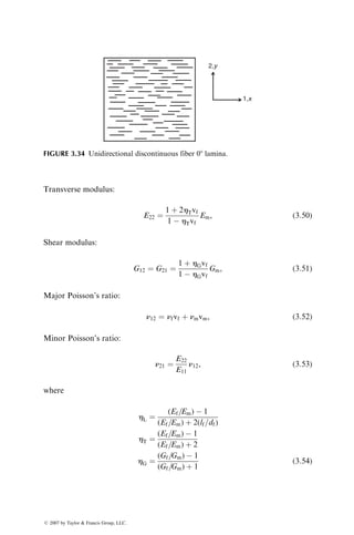
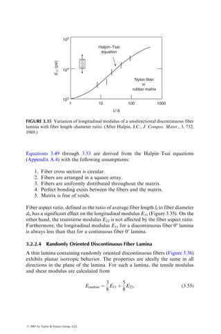
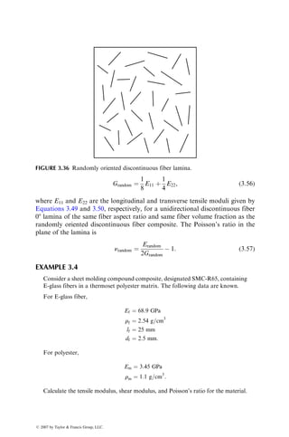
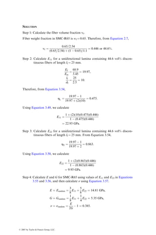
![3.2.3 COEFFICIENTS OF LINEAR THERMAL EXPANSION [21]
For a unidirectional continuous fiber lamina, coefficients of linear thermal
expansion in the 08 and 908 directions can be calculated from the following
equations:
a11 ¼
aflEfvf þ amEmvm
Efvf þ Emvm
(3:58)
and
a22 ¼ (1 þ nf)
(afl þ afr)
2
vf þ (1 þ nm)amvm a11n12, (3:59)
where
n12 ¼ nfvf þ nmvm
afl ¼ coefficient of linear thermal expansion for the fiber in the longitudinal
direction
afr ¼ coefficient of linear thermal expansion for the fiber in the radial direction
am ¼ coefficient of linear thermal expansion for the matrix
Equations 3.58 and 3.59 are plotted in Figure 3.37 as a function of fiber volume
fraction for a typical glass fiber-reinforced polymer matrix composite for which
am af. It should be noted that the coefficient of linear thermal expansion in
such composites is greater in the transverse (908) direction than in the longitu-
dinal (08) direction.
If the fibers are at an angle u with the x direction, the coefficients of thermal
expansion in the x and y directions can be calculated using a11 and a22:
am
a11
af
1
0
vf
a22
2
1
a
FIGURE 3.37 Variation of longitudinal and transverse coefficients of thermal expansion
with fiber volume fraction in a 08 unidirectional continuous E-glass fiber-reinforced
epoxy lamina.
ß 2007 by Taylor Francis Group, LLC.](https://image.slidesharecdn.com/fiberreinforcedcompositesmaterialsmanufacturinganddesignp1-220510152925-9ef3de0d/85/Fiber_Reinforced_Composites_Materials_Manufacturing_and_Design_P-1-pdf-184-320.jpg)
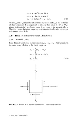
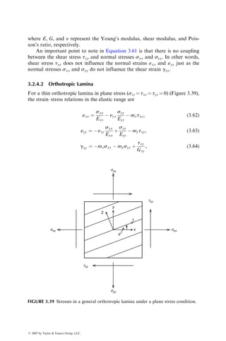
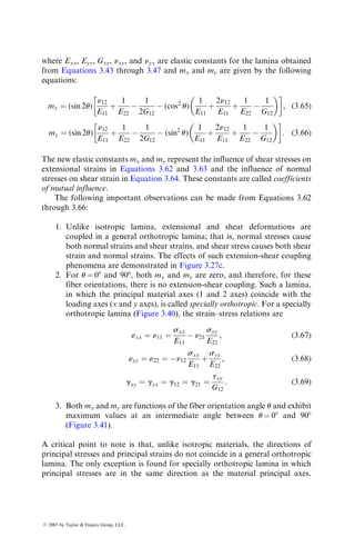
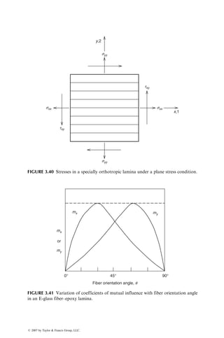
![Greszczuk [22] has shown that the difference between the principal stress and
principal strain directions is a function of the material orthotropy (i.e., the ratio
E11=E22) as well as the ratio of the two principal stresses (i.e., the ratio s2=s1,
Figure 3.42).
EXAMPLE 3.5
A thin plate is subjected to a biaxial stress field of sxx ¼ 1 GPa and syy ¼ 0.5 GPa.
Calculate the strains in the xy directions if the plate is made of (a) steel, (b) a 08
unidirectional boron–epoxy composite, and (c) a 458 unidirectional boron–epoxy
composite.
Use the elastic properties of the boron–epoxy composite given in Appendix A.5.
0
0
10
20
30
40
50
60
15
Angular
difference
in
principal
stress
and
principal
strain
directions
(degrees)
30 45
0.0
0.1
0.2
0.3
sxx
q
syy /sxx
syy
x
1
y
Principal strain
direction
60
Fiber orientation angle, q (degrees)
75 90
FIGURE 3.42 Difference in principal stress and principal strain directions as a function
of fiber orientation angle in an E-glass–epoxy composite (E11=E22 ¼ 2.98). Note that,
for the biaxial normal stress condition shown in this figure, sxx and syy represent the
principal stresses s1 and s2, respectively. (After Greszczuk, L.B., Orientation Effects in
the Mechanical Behavior of Anisotropic Structural Materials, ASTM STP, 405, 1, 1966.)
ß 2007 by Taylor Francis Group, LLC.](https://image.slidesharecdn.com/fiberreinforcedcompositesmaterialsmanufacturinganddesignp1-220510152925-9ef3de0d/85/Fiber_Reinforced_Composites_Materials_Manufacturing_and_Design_P-1-pdf-189-320.jpg)
![SOLUTION
1. Using E ¼ 207 GPa and n ¼ 0.33 for steel in Equation 3.61, we obtain
«xx ¼
1
207
[1 (0:33) (0:5)] ¼ 4:034 103
,
«yy ¼
1
207
[ (0:33) (1) þ 0:5] ¼ 0:821 103
,
gxy ¼ 0:
2. For the 08 unidirectional boron–epoxy (from Appendix A.5):
E11 ¼ 207 GPa (same as steel’s modulus)
E22 ¼ 19 GPa
n12 ¼ 0:21
G12 ¼ 6:4 GPa:
We first calculate n21:
n21 ¼ (0:21)
19
207
¼ 0:0193:
Since 08 unidirectional boron–epoxy is a specially orthotropic lamina, we
use Equations 3.67 through 3.69 to obtain
«xx ¼
1
207
(0:0193)
0:5
19
¼ 4:323 103
,
«yy ¼ (0:21)
1
207
þ
0:5
19
¼ 25:302 103
,
gxy ¼ 0:
3. We first need to calculate the elastic constants of the 458 boron–epoxy
laminate using Equations 3.43 through 3.47:
Exx ¼ Eyy ¼ 18:896 GPa,
nxy ¼ nyx ¼ 0:476:
Next, we calculate the coefficients of mutual influence using Equations
3.65 and 3.66:
mx ¼ my ¼ 0:0239 GPa1
:
ß 2007 by Taylor Francis Group, LLC.](https://image.slidesharecdn.com/fiberreinforcedcompositesmaterialsmanufacturinganddesignp1-220510152925-9ef3de0d/85/Fiber_Reinforced_Composites_Materials_Manufacturing_and_Design_P-1-pdf-190-320.jpg)
![Now, we use Equations 3.62 through 3.64 to calculate:
«xx ¼
1
18:896
(0:476)
0:5
18:896
¼ 40:326 103
,
«yy ¼ (0:476)
1
18:896
þ
0:5
18:896
¼ 1:270 103
,
gxy ¼ (0:0239) (1 þ 0:5) ¼ 35:85 103
:
Note that although the shear stress is zero, there is a shear strain due to
extension-shear coupling. This causes a distortion of the plate in addition
to the extensions due to «xx and «yy as shown in the figure. In addition,
note that a negative shear strain means that the initial 908 angle between
the adjacent edges of the stress element is increased.
sxx = 1 GPa
syy = 0.5 GPa
sxx = 1 GPa
syy = 0.5 GPa
y
x
(a) Steel (b) 08 Boron fiber–epoxy (c) 458 Boron fiber–epoxy
3.2.5 COMPLIANCE AND STIFFNESS MATRICES
3.2.5.1 Isotropic Lamina
For an isotropic lamina, Equation 3.61 can be written in the matrix form as
«xx
«yy
gxy
2
6
4
3
7
5 ¼
1
E n
E 0
n
E
1
E 0
0 0 1
G
2
6
4
3
7
5
sxx
syy
txy
2
4
3
5 ¼ [S]
sxx
syy
txy
2
4
3
5, (3:70)
ß 2007 by Taylor Francis Group, LLC.](https://image.slidesharecdn.com/fiberreinforcedcompositesmaterialsmanufacturinganddesignp1-220510152925-9ef3de0d/85/Fiber_Reinforced_Composites_Materials_Manufacturing_and_Design_P-1-pdf-191-320.jpg)
![where [S] represents the compliance matrix relating strains to known stresses.
The inverse of the compliance matrix is called the stiffness matrix, which is used
in relating stresses to known strains. Thus, the stiffness matrix [Q] for an
isotropic lamina is
[Q] ¼ [S]1
¼
E
1n2
nE
1n2 0
nE
1n2
E
1n2 0
0 0 G
2
6
4
3
7
5: (3:71)
3.2.5.2 Specially Orthotropic Lamina (u508 or 908)
Arranging Equations 3.67 through 3.69 in matrix form, we can write the strain–
stress relation for a specially orthotropic lamina as
«xx
«yy
gxy
2
6
4
3
7
5 ¼
S11 S12 0
S21(¼S12) S22 0
0 0 S66
2
4
3
5
sxx
syy
txy
2
4
3
5 ¼ [S]
sxx
syy
txy
2
4
3
5, (3:72)
where
S11 ¼
1
E11
S12 ¼ S21 ¼
n12
E11
¼
n21
E22
S22 ¼
1
E22
S66 ¼
1
G12
(3:73)
The [S] matrix is the compliance matrix for the specially orthotropic lamina.
Inverting Equation 3.72, we can write the stress–strain relations for a specially
orthotropic lamina as
sxx
syy
txy
2
4
3
5 ¼
Q11 Q12 0
Q21(¼ Q12) Q22 0
0 0 Q66
2
4
3
5
«xx
«yy
gxy
2
6
4
3
7
5 ¼ [Q]
«xx
«yy
gxy
2
6
4
3
7
5, (3:74)
where [Q] represents the stiffness matrix for the specially orthotropic lamina.
Various elements in the [Q] matrix are
ß 2007 by Taylor Francis Group, LLC.](https://image.slidesharecdn.com/fiberreinforcedcompositesmaterialsmanufacturinganddesignp1-220510152925-9ef3de0d/85/Fiber_Reinforced_Composites_Materials_Manufacturing_and_Design_P-1-pdf-192-320.jpg)
![Q11 ¼
E11
1 n12n21
,
Q22 ¼
E22
1 n12n21
,
Q12 ¼ Q21 ¼
n12E22
1 n12n21
¼
n21E11
1 n12n21
,
Q66 ¼ G12: (3:75)
3.2.5.3 General Orthotropic Lamina (u 6¼ 08 or 908)
The strain–stress relations for a general orthotropic lamina, Equations 3.62
through 3.64, can be expressed in matrix notation as
«xx
«yy
gxy
2
4
3
5 ¼
S11
S12
S16
S12
S22
S26
S16
S26
S66
2
4
3
5
sxx
syy
txy
2
4
3
5 ¼ [
S]
sxx
syy
txy
2
4
3
5, (3:76)
where [
S] represents the compliance matrix for the lamina. Various elements in
the [
S] matrix are expressed in terms of the elements in the [S] matrix for a
specially orthotropic lamina. These expressions are
S11 ¼
1
Exx
¼ S11 cos4
u þ (2S12 þ S66) sin2
u cos2
u þ S22 sin4
u,
S12 ¼
nxy
Exx
¼ S12(sin4
u þ cos4
u) þ (S11 þ S22 S66) sin2
u cos2
u,
S22 ¼
1
Eyy
¼ S11 sin4
u þ (2S12 þ S66) sin2
u cos2
u þ S22 cos4
u,
S16 ¼ mx ¼ (2S11 2S12 S66) sin u cos3
u (2S22 2S12 S66) sin3
u cos u,
S26 ¼ my ¼ (2S11 2S12 S66) sin3
u cos u (2S22 2S12 S66) sin u cos3
u,
S66 ¼
1
Gxy
¼ 2(2S11 þ 2S22 4S12 S66) sin2
u cos2
u þ S66(sin4
u þ cos4
u):
(3:77)
On substitution for S11, S12, and so on, into Equation 3.77, we obtain the same
equations as Equations 3.43 through 3.46 for Exx, Eyy, Gxy, and nxy, and
Equations 3.65 and 3.66 for mx and my.
Inverting Equation 3.76, the stress–strain relations for a general orthotropic
lamina can be written as
sxx
syy
txy
2
4
3
5 ¼
Q11
Q12
Q16
Q12
Q22
Q26
Q16
Q26
Q66
2
4
3
5
«xx
«yy
gxy
2
4
3
5 ¼ [
Q]
sxx
syy
gxy
2
4
3
5, (3:78)
ß 2007 by Taylor Francis Group, LLC.](https://image.slidesharecdn.com/fiberreinforcedcompositesmaterialsmanufacturinganddesignp1-220510152925-9ef3de0d/85/Fiber_Reinforced_Composites_Materials_Manufacturing_and_Design_P-1-pdf-193-320.jpg)
![where [
Q] represents the stiffness matrix for the lamina. Various elements in the
[
Q] matrix are expressed in terms of the elements in the [Q] matrix as
Q11 ¼ Q11 cos4
u þ 2(Q12 þ 2Q66) sin2
u cos2
u þ Q22 sin4
u,
Q12 ¼ Q12(sin4
u þ cos4
u) þ (Q11 þ Q22 4Q66) sin2
u cos2
u,
Q22 ¼ Q11 sin4
u þ 2(Q12 þ 2Q66) sin2
u cos2
u þ Q22 cos4
u,
Q16 ¼ (Q11 Q12 2Q66) sin u cos3
u þ (Q12 Q22 þ 2Q66) sin3
u cos u,
Q26 ¼ (Q11 Q12 2Q66) sin3
u cos u þ (Q12 Q22 þ 2Q66) sin u cos3
u,
Q66 ¼ (Q11 þ Q22 2Q12 2Q66) sin2
u cos2
u þ Q66(sin4
u þ cos4
u): (3:79)
In using Equations 3.77 and 3.79, the following points should be noted:
1. Elements
S16 and
S26 in the [
S] matrix or
Q16 and
Q26 in the [
Q] matrix
represent extension-shear coupling.
2. From Equation 3.77 or 3.79, it appears that there are six elastic con-
stants that govern the stress–strain behavior of a lamina. However, a
closer examination of these equations would indicate that
S16 and
S26
(or
Q16 and
Q26) are linear combinations of the four basic elastic con-
stants, namely,
S11,
S12,
S22, and
S66, and therefore are not independent.
3. Elements in both the [
S] and [
Q] matrices are expressed in terms of the
properties in the principal material directions, namely, E11, E22, G12, and
n12, which can be either experimentally determined or predicted from the
constituent properties using Equations 3.36 through 3.40.
4. Elements in the [
Q] and [
S] matrices can be expressed in terms of five
invariant properties of the lamina, as shown below.
Using trigonometric identities, Tsai and Pagano [23] have shown that the
elements in the [
Q] matrix can be written as
Q11 ¼ U1 þ U2 cos 2u þ U3 cos 4u,
Q12 ¼
Q21 ¼ U4 U3 cos 4u,
Q22 ¼ U1 U2 cos 2u þ U3 cos 4u,
Q16 ¼
1
2
U2 sin 2u þ U3 sin 4u,
Q26 ¼
1
2
U2 sin 2u U3 sin 4u,
Q66 ¼ U5 U3 cos 4u, (3:80)
where U1 through U5 represent angle-invariant stiffness properties of a lamina
and are given as
ß 2007 by Taylor Francis Group, LLC.](https://image.slidesharecdn.com/fiberreinforcedcompositesmaterialsmanufacturinganddesignp1-220510152925-9ef3de0d/85/Fiber_Reinforced_Composites_Materials_Manufacturing_and_Design_P-1-pdf-194-320.jpg)
![U1 ¼
1
8
(3Q11 þ 3Q22 þ 2Q12 þ 4Q66),
U2 ¼
1
2
(Q11 Q22),
U3 ¼
1
8
(Q11 þ Q22 2Q12 4Q66),
U4 ¼
1
8
(Q11 þ Q22 þ 6Q12 4Q66),
U5 ¼
1
2
(U1 U4): (3:81)
It is easy to observe from Equation 3.80 that for fiber orientation angles u and u,
Q11(u) ¼
Q11(u),
Q12(u) ¼
Q12(u),
Q22(u) ¼
Q22(u),
Q66(u) ¼
Q66(u),
Q16(u) ¼
Q16(u),
Q26(u) ¼
Q26(u):
Similar expressions for the elements in the [
S] matrix are
S11 ¼ V1 þ V2 cos 2u þ V3 cos 4u,
S12 ¼
S21 ¼ V4 V3 cos 4u,
S22 ¼ V1 V2 cos 2u þ V3 cos 4u,
S16 ¼ V2 sin 2u þ 2V3 sin 4u,
S26 ¼ V2 sin 2u 2V3 sin 4u,
S66 ¼ V5 4V3 cos 4u, (3:82)
where
V1 ¼
1
8
(3S11 þ 3S22 þ 2S12 þ S66),
V2 ¼
1
2
(S11 S22),
V3 ¼
1
8
(S11 þ S22 2S12 S66),
V4 ¼
1
8
(S11 þ S22 þ 6S12 S66),
V5 ¼ 2(V1 V4): (3:83)
These invariant forms are very useful in computing the elements in [
Q] and [
S]
matrices for a lamina.
ß 2007 by Taylor Francis Group, LLC.](https://image.slidesharecdn.com/fiberreinforcedcompositesmaterialsmanufacturinganddesignp1-220510152925-9ef3de0d/85/Fiber_Reinforced_Composites_Materials_Manufacturing_and_Design_P-1-pdf-195-320.jpg)
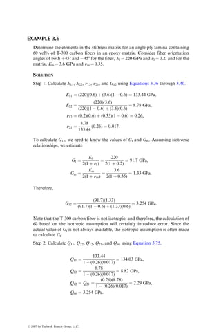
![Step 3: Calculate U1, U2, U3, U4, and U5 using Equation 3.81.
U1 ¼
1
8
[(3)(134:03) þ (3)(8:82) þ (2)(2:29) þ (4)(3:254)] ¼ 55:77 GPa,
U2 ¼
1
2
(134:03 8:82) ¼ 62:6 GPa,
U3 ¼
1
8
[134:03 þ 8:82 (2)(2:29) (4)(3:254)] ¼ 15:66 GPa,
U4 ¼
1
8
[134:03 þ 8:82 þ (6)(2:29) (4)(3:259)] ¼ 17:95 GPa,
U5 ¼
1
2
(55:77 17:95) ¼ 18:91 GPa:
Step 4: Calculate
Q11,
Q22,
Q12,
Q16,
Q26, and
Q66 using Equation 3.80. For a
u ¼ þ458 lamina,
Q11 ¼ 55:77 þ (62:6) cos 90
þ (15:66) cos 180
¼ 40:11 GPa,
Q22 ¼ 55:77 (62:6) cos 90
þ (15:66) cos 180
¼ 40:11 GPa,
Q12 ¼ 17:95 (15:66) cos 180
¼ 33:61 GPa,
Q66 ¼ 18:91 (15:66) cos 180
¼ 34:57 GPa,
Q16 ¼
1
2
(62:6) sin 90
þ (15:66) sin 180
¼ 31:3 GPa,
Q26 ¼
1
2
(62:6) sin 90
(15:66) sin 180
¼ 31:3 GPa:
Similarly, for a u ¼ 458 lamina,
Q11 ¼ 40:11 GPa,
Q22 ¼ 40:11 GPa,
Q12 ¼ 33:61 GPa,
Q66 ¼ 34:57 GPa,
Q16 ¼ 31:3 GPa,
Q26 ¼ 31:3 GPa:
In the matrix form,
[
Q]45 ¼
40:11 33:61 31:3
33:61 40:11 31:3
31:3 31:3 34:57
2
4
3
5 GPa,
[
Q]45 ¼
40:11 33:61 31:3
33:61 40:11 31:3
31:3 31:3 34:57
2
4
3
5 GPa:
ß 2007 by Taylor Francis Group, LLC.](https://image.slidesharecdn.com/fiberreinforcedcompositesmaterialsmanufacturinganddesignp1-220510152925-9ef3de0d/85/Fiber_Reinforced_Composites_Materials_Manufacturing_and_Design_P-1-pdf-197-320.jpg)
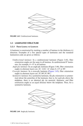
![u(z) ¼ u(z),
where z is the distance from the midplane of the laminate. Some examples
of symmetric laminates and their codes are listed.
1 2 3 4 5 6
1. [0=þ45=90=90 þ45=0]
Code: [0=45=90]S
Subscript S in the code indicates symmetry about the midplane.
1 2 3 4 5
2. [0=þ45=90=þ45=0]
Code: [0=45=90]S
The bar over 90 indicates that the plane of symmetry passes midway
through the thickness of the 908 lamina.
1 2 3 4 5 6 7
3. [0=þ45=45=90=45=þ45=0]
Code: [0=+45=90]S
Adjacent þ458 and 458 laminas are grouped as ±458.
1 2 3 4 5 6 7 8 9 10 11 12 13 14
4. [0 = 90 = 0 = 0 = 0 = 0 = 45 = 45 = 0 = 0 = 0 = 0 = 90 = 0]
Code: [0=90=04=45]S
Four adjacent 08 plies are grouped together as 04.
1 2 3 4 5 6 7 8 9 10
5. [0=45=45=þ45=45=45=þ45=45=þ45=0]
Code: [0=(±45)2]S
Two adjacent ±458 plies are grouped as (±45)2.
FIGURE 3.45 Cross-ply laminate.
ß 2007 by Taylor Francis Group, LLC.](https://image.slidesharecdn.com/fiberreinforcedcompositesmaterialsmanufacturinganddesignp1-220510152925-9ef3de0d/85/Fiber_Reinforced_Composites_Materials_Manufacturing_and_Design_P-1-pdf-199-320.jpg)
![6. [0=45=45=45=45=45=45=0=0=0=0=0=45=45=45=45=45=45=0]
Code: [0=(+45)3=02=
0]S
7. [u=u=u=u=u=u=u=u]
Code: [u= u]2S or [±u]2S
Two adjacent ±u plies on each side of the plane of symmetry are denoted
by the subscript 2S.
8. Symmetric angle-ply laminate
[u= u= u=u=u=u=u]
Code: [u=u=
u]S
Note that symmetric angle-ply laminates contain an odd number of plies.
9. Symmetric cross-ply laminate
[0=90=0=90=0=90=0=90=0]
Code: [(0=90)2=
0]S
Note that symmetric cross-ply laminates contain an odd number of plies.
10. Hybrid (interply) laminate.
[0B=0B=45C=45C=90G=90G=45C=45C=0B=0B]
Code: [02B=(±45)C=90G]S
where B, C, and G represent boron, carbon, and glass fiber, respectively.
Antisymmetric laminate: In antisymmetric laminates, the ply orientation is
antisymmetric about the centerline of the laminate; that is, for each ply of
fiber orientation angle u above the midplane, there is a ply of fiber
orientation angle u with identical material and thickness at an equal
distance below the midplane. Thus, for an antisymmetric laminate,
u(z) ¼ u(z):
For example, u= u= u = u is an antisymmetric laminate. In contrast,
u=u= u=u is symmetric.
Unsymmetric laminate: In unsymmetric laminates, there is no symmetry or
antisymmetry. Examples are 0=0=0=90=90=90 and 0=u=u=90.
Quasi-isotropic laminate: These laminates are made of three or more laminas
of identical thickness and material with equal angles between each
adjacent lamina. Thus, if the total number of laminas is n, the orientation
angles of the laminas are at increments of p=n. The resulting laminate
ß 2007 by Taylor Francis Group, LLC.](https://image.slidesharecdn.com/fiberreinforcedcompositesmaterialsmanufacturinganddesignp1-220510152925-9ef3de0d/85/Fiber_Reinforced_Composites_Materials_Manufacturing_and_Design_P-1-pdf-200-320.jpg)
![exhibits an in-plane isotropic elastic behavior in the xy plane. However,
its strength properties may still vary with the direction of loading.
Examples of simple quasi-isotropic laminates are [þ60=0=60] and
[þ45=0=45=90]. Other combinations of these stacking sequences, such
as [0=þ60=60] and [0=þ45=45=90], also exhibit in-plane isotropic
elastic behavior. A very common and widely used quasi-isotropic sym-
metrical stacking sequence is [0=±45=90]S.
3.3.2 LAMINATION THEORY
Lamination theory is useful in calculating stresses and strains in each lamina of
a thin laminated structure. Beginning with the stiffness matrix of each lamina,
the step-by-step procedure in lamination theory includes
1. Calculation of stiffness matrices for the laminate
2. Calculation of midplane strains and curvatures for the laminate due to a
given set of applied forces and moments
3. Calculation of in-plane strains «xx, «yy, and gxy for each lamina
4. Calculation of in-plane stresses sxx, syy, and txy in each lamina
The derivation of lamination theory is given in Ref. [16]. The principal equa-
tions and a number of examples are presented in the following sections.
3.3.2.1 Assumptions
Basic assumptions in the lamination theory are
1. Laminate is thin and wide (width thickness).
2. A perfect interlaminar bond exists between various laminas.
3. Strain distribution in the thickness direction is linear.
4. All laminas are macroscopically homogeneous and behave in a linearly
elastic manner.
The geometric midplane of the laminate contains the xy axes, and the z
axis defines the thickness direction. The total thickness of the laminate is h,
and the thickness of various laminas are represented by t1, t2, t3, and so on.
The total number of laminas is N. A sketch for the laminate is shown in
Figure 3.46.
3.3.2.2 Laminate Strains
Following assumption 3, laminate strains are linearly related to the distance
from the midplane as
ß 2007 by Taylor Francis Group, LLC.](https://image.slidesharecdn.com/fiberreinforcedcompositesmaterialsmanufacturinganddesignp1-220510152925-9ef3de0d/85/Fiber_Reinforced_Composites_Materials_Manufacturing_and_Design_P-1-pdf-201-320.jpg)
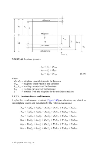
![In matrix notation,
Nxx
Nyy
Nxy
2
4
3
5 ¼ [A]
«
xx
«
yy
g
xy
2
4
3
5 þ [B]
kxx
kyy
kxy
2
4
3
5 (3:85)
and
Mxx
Myy
Mxy
2
4
3
5 ¼ [B]
«
xx
«
yy
g
xy
2
4
3
5 þ [D]
kxx
kyy
kxy
2
4
3
5, (3:86)
where
Nxx ¼ normal force resultant in the x direction (per unit width)
Nyy ¼ normal force resultant in the y direction (per unit width)
Nxy ¼ shear force resultant (per unit width)
Mxx ¼ bending moment resultant in the yz plane (per unit width)
Myy ¼ bending moment resultant in the xz plane (per unit width)
Mxy ¼ twisting moment (torsion) resultant (per unit width)
[A] ¼ extensional stiffness matrix for the laminate (unit: N=m or lb=in.)
[A] ¼
A11 A12 A16
A12 A22 A26
A16 A26 A66
2
4
3
5, (3:87)
[B] ¼ coupling stiffness matrix for the laminate (unit: N or lb)
[B] ¼
B11 B12 B16
B12 B22 B26
B16 B26 B66
2
4
3
5, (3:88)
Nxx Nxx
Nyy
Nyy
Mxy
Myx = Mxy
Myy
Myy
Mxx
Mxx Mxy
Myx
y
z
x
Nyx = Nxy
Nxy
FIGURE 3.47 In-plane, bending, and twisting loads applied on a laminate.
ß 2007 by Taylor Francis Group, LLC.](https://image.slidesharecdn.com/fiberreinforcedcompositesmaterialsmanufacturinganddesignp1-220510152925-9ef3de0d/85/Fiber_Reinforced_Composites_Materials_Manufacturing_and_Design_P-1-pdf-203-320.jpg)
![[D] ¼ bending stiffness matrix for the laminate (unit: N m or lb in.)
[D] ¼
D11 D12 D16
D12 D22 D26
D16 D26 D66
2
4
3
5: (3:89)
Referring to Equation 3.85, it can be observed that
1. A16 and A26 couple in-plane normal forces to midplane shear strain and
in-plane shear force to midplane normal strains.
2. B11, B12, and B22 couple in-plane normal forces to bending curvatures
and bending moments to midplane normal strains.
3. B16 and B26 couple in-plane normal forces to twisting curvature and
twisting moment to midplane normal strains.
4. B66 couples in-plane shear force to twisting curvature and twisting
moment to midplane shear strain.
5. D16 and D26 couple bending moments to twisting curvature and twisting
moment to bending curvatures.
The couplings between normal forces and shear strains, bending moments
and twisting curvatures, and so on, occur only in laminated structures and
not in a monolithic structure. If the laminate is properly constructed, some of
these couplings can be eliminated. For example, if the laminate is constructed
such that both A16 and A26 ¼ 0, there will be no coupling between in-plane
normal forces and midplane shear strains, that is, in-plane normal forces will
not cause shear deformation of the laminate. Similarly, if the laminate is
constructed such that both D16 and D26 ¼ 0, there will be coupling between
bending moments and twisting curvature, that is, bending moments will not
cause twisting of the laminate. These special constructions are described in the
following section.
3.3.2.4 Elements in Stiffness Matrices
The elements in [A], [B], and [D] matrices are calculated from
Amn ¼
X
N
j¼1
Qmn
j
hj hj1
, (3:90)
Bmn ¼
1
2
X
N
j¼1
Qmn
j
h2
j h2
j1
, (3:91)
ß 2007 by Taylor Francis Group, LLC.](https://image.slidesharecdn.com/fiberreinforcedcompositesmaterialsmanufacturinganddesignp1-220510152925-9ef3de0d/85/Fiber_Reinforced_Composites_Materials_Manufacturing_and_Design_P-1-pdf-204-320.jpg)
![Dmn ¼
1
3
X
N
j¼1
Qmn
j
h3
j h3
j1
, (3:92)
where
N ¼ total number of laminas in the laminate
(
Qmn)j ¼ elements in the [
Q] matrix of the jth lamina
hj1 ¼ distance from the midplane to the top of the jth lamina
hj ¼ distance from the midplane to the bottom of the jth lamina
For the coordinate system shown in Figure 3.46, hj is positive below the mid-
plane and negative above the midplane.
The elements of the stiffness matrices [A], [B], and [D] are functions of the
elastic properties of each lamina and its location with respect to the midplane of
the laminate. The following observations are important regarding these stiff-
ness matrices:
1. If [B] is a nonzero matrix, a normal force, such as Nxx, will create
extension and shear deformations as well as bending–twisting curva-
tures. Similarly, a bending moment, such as Mxx, will create bending and
twisting curvatures as well as extension-shear deformations. Such
‘‘extension-bending coupling,’’ represented by the [B] matrix, is unique
in laminated structures regardless of whether the layers are isotropic or
orthotropic. The coupling occurs because of the stacking of layers.
2. For a symmetric laminate, [B] ¼ [0] and there is no extension-bending
coupling. To construct a symmetric laminate, every lamina of þu
orientation above the midplane must be matched with an identical (in
thickness and material) lamina of þu orientation at the same distance
below the midplane (Figure 3.48). Note that a symmetric angle-ply or
cross-ply laminate contains an odd number of plies.
t0
t0
Midplane
h1
h1
+q
+q
FIGURE 3.48 Symmetric laminate configuration for which [B] ¼ [0], and therefore no
extension-bending coupling.
ß 2007 by Taylor Francis Group, LLC.](https://image.slidesharecdn.com/fiberreinforcedcompositesmaterialsmanufacturinganddesignp1-220510152925-9ef3de0d/85/Fiber_Reinforced_Composites_Materials_Manufacturing_and_Design_P-1-pdf-205-320.jpg)
![3. If for every lamina of þu orientation, there is an identical (equal in
thickness and material) lamina of u orientation (Figure 3.49), the
normal stress–shear strain coupling (represented by A16 and A26 in
the [A] matrix) for the laminate is zero. The locations of these
two laminas are arbitrary. Such a laminate is called balanced;
for example, [0=þ30=30=þ30=30=0] is a balanced laminate for
which A16 ¼ A26 ¼ 0. Note that, with proper positioning of layers, it
is possible to prepare a balanced symmetric laminate. For example,
[0=þ30=30=30=þ30=0] is a balanced symmetric laminate, for which
A16 ¼ A26 ¼ 0 as well as [B] ¼ [0].
4. If for every lamina of þu orientation above the midplane, there is
an identical lamina (in thickness and material) of u orientation at
the same distance below the midplane (Figure 3.50), the bending
Midplane
+q
−q
t0
t0
h2
h1
FIGURE 3.49 Balanced laminate configuration for which A16 ¼ A26 ¼ 0, and therefore
no extension-shear coupling.
Midplane
+q
−q
t0
t0
h1
h1
FIGURE 3.50 Laminate configuration for which D16 ¼ D26 ¼ 0, and therefore no bend-
ing-twisting coupling.
ß 2007 by Taylor Francis Group, LLC.](https://image.slidesharecdn.com/fiberreinforcedcompositesmaterialsmanufacturinganddesignp1-220510152925-9ef3de0d/85/Fiber_Reinforced_Composites_Materials_Manufacturing_and_Design_P-1-pdf-206-320.jpg)
![moment-twisting curvature coupling (represented by D16 and D26
in the [D] matrix) for the laminate is zero. For example, for a
[0=þ30=30=þ30=30=0] laminate, D16 ¼ D26 ¼ 0. Note that the D16
and D26 terms cannot be zero for a symmetric laminate, unless u ¼ 08
and 908.
EXAMPLE 3.7
Determine [A], [B], and [D] matrices for (a) a [þ45=45] angle-ply laminate, (b) a
[þ45=45]S symmetric laminate, and (c) a [þ45=0=45] unsymmetric laminate.
Each lamina is 6 mm thick and contains 60 vol% of T-300 carbon fiber in an epoxy
matrix. Use the same material properties as in Example 3.6.
Laminated structure
Mid
plane
(a)
Mid
plane
(b)
h0
h0
h0
h2
h2
h4
h2
h1
h1
h3
−h3
+z
+z
+z
(1) +45⬚
(2) −45⬚
(1) +45⬚
(4) +45⬚
(2) −45⬚
(1) +45⬚
(2) 0⬚
(3) −45⬚
(3) −45⬚
−h1
Mid
plane
(c)
SOLUTION
From Example 3.6, [
Q] matrices for the 08, þ458, and 458 layers are written as
[
Q]0 ¼ [Q]0 ¼
134:03 2:29 0
2:29 8:82 0
0 0 3:254
2
6
6
4
3
7
7
5GPa,
[
Q]þ45 ¼
40:11 33:61 31:3
33:61 40:11 31:3
31:3 31:3 34:57
2
6
6
4
3
7
7
5 GPa,
[
Q]45 ¼
40:11 33:61 31:3
33:61 40:11 31:3
31:3 31:3 34:57
2
6
6
4
3
7
7
5 GPa:
ß 2007 by Taylor Francis Group, LLC.](https://image.slidesharecdn.com/fiberreinforcedcompositesmaterialsmanufacturinganddesignp1-220510152925-9ef3de0d/85/Fiber_Reinforced_Composites_Materials_Manufacturing_and_Design_P-1-pdf-207-320.jpg)
![(a) [þ45=45] Angle-ply laminate: From the figure (top left), we note
h0 ¼ 0.006 m, h1 ¼ 0, and h2 ¼ 0.006 m. In this laminate, (
Qmn)1 ¼
(
Qmn)þ458 and (
Qmn)2 ¼ (
Qmn)458. Therefore,
Amn ¼ (
Qmn)1(h1 h0) þ (
Qmn)2(h2 h1)
¼ 6 103
(
Qmn)þ45 þ 6 103
(
Qmn)45 ,
Bmn ¼
1
2
(
Qmn)1 h2
1 h2
0
þ (
Qmn)2 h2
2 h2
1](https://image.slidesharecdn.com/fiberreinforcedcompositesmaterialsmanufacturinganddesignp1-220510152925-9ef3de0d/85/Fiber_Reinforced_Composites_Materials_Manufacturing_and_Design_P-1-pdf-208-320.jpg)
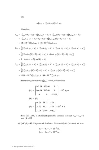
![¼ 72 109
(
Qmn)þ45 þ 72 109
(
Qmn)45 :
Substituting for various (
Qmn) values, we calculate
[A] ¼
481:32 403:32 0
403:32 481:32 0
0 0 414:84
2
6
6
6
4
3
7
7
7
5
106
N=m,
[B] ¼
0 0 1126:8
0 0 1126:8
1126:8 1126:8 0
2
6
6
6
4
3
7
7
7
5
103
N,
[D] ¼
5775:84 4839:84 0
4839:84 5775:84 0
0 0 4978:08
2
6
6
6
4
3
7
7
7
5
N m:
Note that for a [þ45=45] angle-ply laminate, A16 ¼ A26 ¼ 0 (since it is
balanced) as well as D16 ¼ D26 ¼ 0.
(b) [(45=45)]S Symmetric laminate: From the figure (top right), we note that
h3 ¼ h1 ¼ 0.006 m, h4 ¼ h0 ¼ 0.012 m, and h2 ¼ 0. In this laminate,
(
Qmn)4 ¼ (
Qmn)1 ¼ (
Qmn)þ45
ß 2007 by Taylor Francis Group, LLC.](https://image.slidesharecdn.com/fiberreinforcedcompositesmaterialsmanufacturinganddesignp1-220510152925-9ef3de0d/85/Fiber_Reinforced_Composites_Materials_Manufacturing_and_Design_P-1-pdf-210-320.jpg)

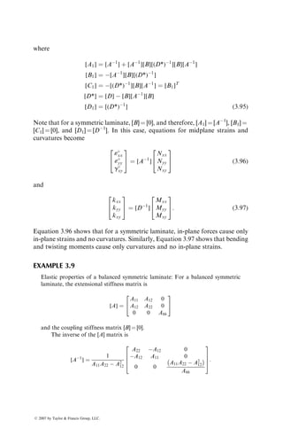
![¼ 1008 109
(
Qmn)þ45 þ 144 109
(
Qmn)45 :
Substituting for various (
Qmn) values, we calculate
[A] ¼
962:64 806:64 0
806:64 962:64 0
0 0 829:68
2
6
6
4
3
7
7
5 106
N=m,
[B] ¼ [0],
[D] ¼
46:21 38:72 27:04
38:72 46:21 27:04
27:04 27:04 39:82
2
6
6
4
3
7
7
5 103
N m:
Note that [±45]S is a balanced symmetric laminate in which A16 ¼ A26 ¼ 0
and [B] ¼ [0].
(c) [þ45=0=45] Unsymmetric laminate: From the figure (bottom), we note
h2 ¼ h1 ¼ 3 103
m,
h3 ¼ h0 ¼ 9 103
m:
ß 2007 by Taylor Francis Group, LLC.](https://image.slidesharecdn.com/fiberreinforcedcompositesmaterialsmanufacturinganddesignp1-220510152925-9ef3de0d/85/Fiber_Reinforced_Composites_Materials_Manufacturing_and_Design_P-1-pdf-215-320.jpg)
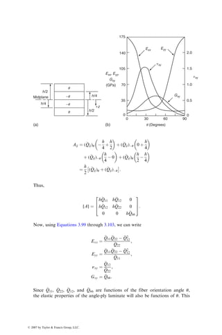
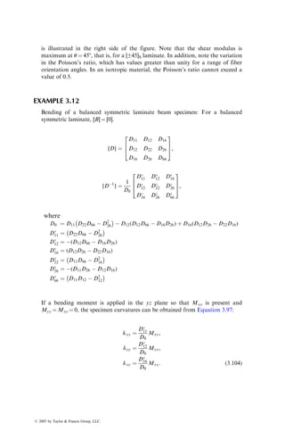
![¼ 234 109
(
Qmn)þ45 þ 18 109
(
Qmn)0 þ 234 109
(
Qmn)45 :
Substituting for [
Qmn] values, we calculate
[A] ¼
1285:50 417:06 0
417:06 534:24 0
0 0 434:36
2
4
3
5 106
N=m,
[B] ¼
0 0 2253:6
0 0 2253:6
2253:6 2253:6 0
2
4
3
5 103
N,
[D] ¼
21,183:84 15,770:70 0
15,770:70 18,930:24 0
0 0 16,237:33
2
4
3
5N m:
Comparing cases (a) and (c), we note that the addition of a 08 lamina
increases the value of A11 by a significant amount, but A12, A22, and A66
are only marginally improved. Elements in the [D] matrix are improved
owing to the presence of the 08 lamina as well as the additional thickness
in the [þ45=0=45] laminate.
EXAMPLE 3.8
Compare the stiffness matrices of [0=90=90=0] and [0=90=0=90] laminates. Assume
each ply has a thickness of h=4.
ß 2007 by Taylor Francis Group, LLC.](https://image.slidesharecdn.com/fiberreinforcedcompositesmaterialsmanufacturinganddesignp1-220510152925-9ef3de0d/85/Fiber_Reinforced_Composites_Materials_Manufacturing_and_Design_P-1-pdf-218-320.jpg)
![0
90
h/2
h/2
h/2
h/2
+z
h/4
h/4
Midplane
h/4
h/4 90
0
(a) (b)
0
90
0
90
SOLUTION
First, we note that for 08 and 908 plies,
(Q11)0 ¼ (Q22)90,
(Q22)0 ¼ (Q11)90,
(Q12)0 ¼ (Q12)90,
(Q66)0 ¼ (Q66)90,
(Q16)0 ¼ (Q16)90 ¼ 0,
(Q26)0 ¼ (Q26)90 ¼ 0:
For the [0=90=90=0] laminate on the left,
Aij ¼ (Qij)0
h
4
h
2
þ (Qij)90 0
h
4
þ (Qij)90
h
4
0
þ (Qij)0
h
2
h
4
¼
h
2
[(Qij)0 þ (Qij)90],
Bij ¼ 0 (since this is a symmetric laminate),
Dij ¼
1
3
(
(Qij)0
h
4
3
h
2
3
#
þ (Qij)90 0
h
4
3
#
þ (Qij)90
h
4
3
0
#
þ (Qij)0
h
2
3
h
4
3
#)
¼
h3
96
[7(Qij)0 þ (Qij)90]:
For the [0=90=0=90] laminate on the right,
ß 2007 by Taylor Francis Group, LLC.](https://image.slidesharecdn.com/fiberreinforcedcompositesmaterialsmanufacturinganddesignp1-220510152925-9ef3de0d/85/Fiber_Reinforced_Composites_Materials_Manufacturing_and_Design_P-1-pdf-219-320.jpg)
![Aij ¼ (Qij)0
h
4
h
2
þ (Qij)90 0
h
4
þ (Qij)0
h
4
0
þ (Qij)90
h
2
h
4
¼
h
2
[(Qij)0 þ (Qij)90],
Bij ¼
1
2
(
(Qij)0
h
4
2
h
2
2
#
þ (Qij)90 0
h
4
2
#
þ (Qij)0
h
4
2
0
#
þ (Qij)90
h
2
2
h
4
2
#)
¼
h2
16
[ (Qij)0 þ (Qij)90],
Dij ¼
1
3
(
(Qij)0
h
4
3
h
2
3
#
þ (Qij)90 0
h
4
3
#
þ (Qij)0
h
4
3
0
#
þ (Qij)90
h
2
3
h
4
3
#)
¼
h3
24
[(Qij)0 þ (Qij)90]:
This example demonstrates the influence of stacking sequence on the stiffness
matrices and the difference it can make to the elastic response of laminates
containing similar plies, but arranged in different orders. In this case, although
[A] matrices for the [0=90=90=0] and [0=90=0=90] are identical, their [B] and [D]
matrices are different.
3.3.2.5 Midplane Strains and Curvatures
If the normal force and moment resultants acting on a laminate are known, its
midplane strains and curvatures can be calculated by inverting Equations 3.85
and 3.86. Thus,
«
xx
«
yy
g
xy
2
4
3
5 ¼ [A1]
Nxx
Nyy
Nxy
2
4
3
5 þ [B1]
Mxx
Myy
Mxy
2
4
3
5 (3:93)
and
kxx
kyy
kxy
2
4
3
5 ¼ [C1]
Nxx
Nyy
Nxy
2
4
3
5 þ [D1]
Mxx
Myy
Mxy
2
4
3
5, (3:94)
ß 2007 by Taylor Francis Group, LLC.](https://image.slidesharecdn.com/fiberreinforcedcompositesmaterialsmanufacturinganddesignp1-220510152925-9ef3de0d/85/Fiber_Reinforced_Composites_Materials_Manufacturing_and_Design_P-1-pdf-220-320.jpg)
![where
[A1] ¼ [A1
] þ [A1
][B][(D*)1
][B][A1
]
[B1] ¼ [A1
][B][(D*)1
]
[C1] ¼ [(D*)1
][B][A1
] ¼ [B1]T
[D*] ¼ [D] [B][A1
][B]
[D1] ¼ [(D*)1
] (3:95)
Note that for a symmetric laminate, [B] ¼ [0], and therefore, [A1] ¼ [A1
], [B1] ¼
[C1] ¼ [0], and [D1] ¼ [D1
]. In this case, equations for midplane strains and
curvatures become
«
xx
«
yy
g
xy
2
4
3
5 ¼ [A1
]
Nxx
Nyy
Nxy
2
4
3
5 (3:96)
and
kxx
kyy
kxy
2
4
3
5 ¼ [D1
]
Mxx
Myy
Mxy
2
4
3
5: (3:97)
Equation 3.96 shows that for a symmetric laminate, in-plane forces cause only
in-plane strains and no curvatures. Similarly, Equation 3.97 shows that bending
and twisting moments cause only curvatures and no in-plane strains.
EXAMPLE 3.9
Elastic properties of a balanced symmetric laminate: For a balanced symmetric
laminate, the extensional stiffness matrix is
[A] ¼
A11 A12 0
A12 A22 0
0 0 A66
2
4
3
5
and the coupling stiffness matrix [B] ¼ [0].
The inverse of the [A] matrix is
[A1
] ¼
1
A11A22 A2
12
A22 A12 0
A12 A11 0
0 0
A11A22 A2
12
A66
2
6
6
4
3
7
7
5:
ß 2007 by Taylor Francis Group, LLC.](https://image.slidesharecdn.com/fiberreinforcedcompositesmaterialsmanufacturinganddesignp1-220510152925-9ef3de0d/85/Fiber_Reinforced_Composites_Materials_Manufacturing_and_Design_P-1-pdf-221-320.jpg)
![Therefore, Equation 3.96 gives
«
xx
«
yy
g
xy
2
4
3
5 ¼
1
A11A22 A2
12
A22 A12 0
A12 A11 0
0 0
A11A22 A2
12
A66
2
6
6
4
3
7
7
5
Nxx
Nyy
Nxy
2
4
3
5: (3:98)
Let us assume that the laminate is subjected to a uniaxial tensile stress sxx in the
x direction, and both syy and txy are zero. If the laminate thickness is h, the tensile
force per unit width in the x direction Nxx ¼ hsxx, Nyy ¼ 0, and Nxy ¼ 0. Thus,
from Equation 3.98, we obtain
«
xx ¼
A22
A11A22 A2
12
hsxx,
«
yy ¼
A12
A11A22 A2
12
hsxx,
g
xy ¼ 0,
which give
Exx ¼
sxx
«
xx
¼
A11A22 A2
12
hA22
, (3:99)
nxy ¼
«
yy
«
xx
¼
A12
A22
: (3:100)
In turn, applying Nyy and Nxy separately, we can determine
Eyy ¼
A11A22 A2
12
hA11
, (3:101)
nyx ¼
A12
A11
which is the same as nxy
Eyy
Exx
, (3:102)
and
Gxy ¼
A66
h
: (3:103)
EXAMPLE 3.10
Elastic properties of a symmetric quasi-isotropic laminate: For a symmetric quasi-
isotropic laminate,
[A] ¼
A11 A12 0
A12 A22 ¼ A11 0
0 0 A66 ¼
A11 A12
2
2
6
4
3
7
5
and [B] ¼ [0]
ß 2007 by Taylor Francis Group, LLC.](https://image.slidesharecdn.com/fiberreinforcedcompositesmaterialsmanufacturinganddesignp1-220510152925-9ef3de0d/85/Fiber_Reinforced_Composites_Materials_Manufacturing_and_Design_P-1-pdf-222-320.jpg)
![Now using the results of Example 3.9, we obtain
Exx ¼ Eyy ¼
A2
11 A2
12
hA11
,
nxy ¼
A12
A11
,
Gxy ¼
A11 A12
2h
,
where h is the laminate thickness.
Note that for a quasi-isotropic laminate, Exx ¼ Eyy and, from the previous
equations, it can be easily shown that
Gxy ¼
Exx
2(1 þ nxy)
:
However, Exx ¼ Eyy does not necessarily mean quasi-isotropy. For example, Exx
and Eyy are equal for a [0=90]S laminate, but it is not a quasi-isotropic laminate.
For a quasi-isotropic laminate, elastic modulus at any arbitrary angle in the plane
of the laminate is the same as Exx or Eyy. That will not be the case with the [0=90]S
laminate.
EXAMPLE 3.11
Elastic properties of symmetric angle-ply laminates: For angled plies with u and
u fiber orientation angles,
Q11(u) ¼
Q11(u),
Q22(u) ¼
Q22(u),
Q12(u) ¼
Q12(u),
Q66(u) ¼
Q66(u),
Q16(u) ¼
Q16(u),
Q26(u) ¼
Q26(u):
Referring to the four-layer angle-ply laminate shown in the left side of the
figure, we can write the elements in the extensional stiffness matrix [A] of the
[u=u]S as
ß 2007 by Taylor Francis Group, LLC.](https://image.slidesharecdn.com/fiberreinforcedcompositesmaterialsmanufacturinganddesignp1-220510152925-9ef3de0d/85/Fiber_Reinforced_Composites_Materials_Manufacturing_and_Design_P-1-pdf-223-320.jpg)
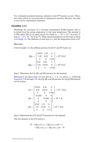
![:
Thus,
[A] ¼
h
Q11 h
Q12 0
h
Q12 h
Q22 0
0 0 h
Q66
2
6
4
3
7
5:
Now, using Equations 3.99 through 3.103, we can write
Exx ¼
Q11
Q22
Q2
12
Q22
,
Eyy ¼
Q11
Q22
Q2
12
Q11
,
nxy ¼
Q12
Q22
,
Gxy ¼
Q66:
Since
Q11,
Q22,
Q12, and
Q66 are functions of the fiber orientation angle u,
the elastic properties of the angle-ply laminate will also be functions of u. This
ß 2007 by Taylor Francis Group, LLC.](https://image.slidesharecdn.com/fiberreinforcedcompositesmaterialsmanufacturinganddesignp1-220510152925-9ef3de0d/85/Fiber_Reinforced_Composites_Materials_Manufacturing_and_Design_P-1-pdf-225-320.jpg)
![is illustrated in the right side of the figure. Note that the shear modulus is
maximum at u ¼ 458, that is, for a [±45]S laminate. In addition, note the variation
in the Poisson’s ratio, which has values greater than unity for a range of fiber
orientation angles. In an isotropic material, the Poisson’s ratio cannot exceed a
value of 0.5.
EXAMPLE 3.12
Bending of a balanced symmetric laminate beam specimen: For a balanced
symmetric laminate, [B] ¼ [0].
[D] ¼
D11 D12 D16
D12 D22 D26
D16 D26 D66
2
6
4
3
7
5,
[D1
] ¼
1
D0
D
11 D
12 D
16
D
12 D
22 D
26
D
16 D
26 D
66
2
6
4
3
7
5,
where
D0 ¼ D11 D22D66 D2
26
D12(D12D66 D16D26) þ D16(D12D26 D22D16)
D
11 ¼ D22D66 D2
26
D
12 ¼ (D12D66 D16D26)
D
16 ¼ (D12D26 D22D16)
D
22 ¼ D11D66 D2
16
D
26 ¼ (D11D26 D12D16)
D
66 ¼ D11D12 D2
12
If a bending moment is applied in the yz plane so that Mxx is present and
Myy ¼ Mxy ¼ 0, the specimen curvatures can be obtained from Equation 3.97:
kxx ¼
D
11
D0
Mxx,
kyy ¼
D
12
D0
Mxx,
kxy ¼
D
16
D0
Mxx: (3:104)
ß 2007 by Taylor Francis Group, LLC.](https://image.slidesharecdn.com/fiberreinforcedcompositesmaterialsmanufacturinganddesignp1-220510152925-9ef3de0d/85/Fiber_Reinforced_Composites_Materials_Manufacturing_and_Design_P-1-pdf-226-320.jpg)
![Thus, even though no twisting moment is applied, the specimen would tend to twist
unless D816 ¼ (D12D26 D22D16) ¼ 0. This is possible only if the balanced symmet-
ric laminate contains fibers in the 08 and 908 directions. The twisting phenomenon
can be easily demonstrated in a three-point flexural test in which the specimen lifts
off the support on opposite corners of its span, as shown in the figure.
3.3.2.6 Lamina Strains and Stresses Due to Applied Loads
Knowing the midplane strains and curvatures for the laminate, strains at the
midplane of each lamina can be calculated using the following linear relationships:
«xx
«yy
gxy
2
4
3
5
j
¼
«
xx
«
yy
g
xy
2
4
3
5 þ zj
kxx
kyy
kxy
2
4
3
5, (3:105)
where zj is the distance from the laminate midplane to the midplane of the jth
lamina.
In turn, stresses in the jth lamina can be calculated using its stiffness matrix.
Thus,
sxx
syy
txy
2
4
3
5
j
¼ [
Qmn]j
«xx
«yy
gxy
2
4
3
5
j
¼ [
Qmn]j
«
xx
«
yy
g
xy
2
4
3
5 þ zj[
Qmn]j
kxx
kyy
kxy
2
4
3
5: (3:106)
Figure 3.51 demonstrates schematically the strain and stress distributions in a
laminate. Note that the strain distribution is continuous and linearly varies
with the distance z from the laminate midplane. The stress distribution is not
continuous, although it varies linearly across each lamina thickness. For thin
laminas, the strain and stress variation across the thickness of each lamina is
small. Therefore, their average values are calculated using the center distance zj,
as shown in Equations 3.105 and 3.106.
ß 2007 by Taylor Francis Group, LLC.](https://image.slidesharecdn.com/fiberreinforcedcompositesmaterialsmanufacturinganddesignp1-220510152925-9ef3de0d/85/Fiber_Reinforced_Composites_Materials_Manufacturing_and_Design_P-1-pdf-227-320.jpg)
![EXAMPLE 3.13
Calculate lamina stresses at the midplane of each lamina in the [þ45=45]
laminate in Example 3.7 due to Nxx ¼ 100 kN=m.
SOLUTION
Step 1: From the laminate stiffness matrices [A], [B], and [D], determine [A1
],
[D*], [A1], [B1], [C1], and [D1].
[A1
] ¼
0:697 0:584 0
0:584 0:697 0
0 0 0:241
2
6
4
3
7
5108
m=N,
[B][A1
][B] ¼
3:06 3:06 0
3:06 3:06 0
0 0 2:87
2
6
4
3
7
5103
N m,
[D*] ¼ [D] [B][A1
][B] ¼
2715:84 1779:84 0
1779:84 2715:84 0
0 0 2108:08
2
6
4
3
7
5N m,
[D1] ¼ [(D*)1
] ¼
6:45 4:23 0
4:23 6:45 0
0 0 4:74
2
6
4
3
7
5104 1
N m
,
[B1] ¼ [A1
][B][(D*)1
] ¼
0 0 603:54
0 0 603:54
602:74 602:74 0
2
6
4
3
7
5109 1
N
,
[C1] ¼ [(D*)1
][B][A1
] ¼
0 0 602:74
0 0 602:74
603:54 603:54 0
2
6
4
3
7
5109 1
N
,
x
Nxx
Mxx
h
z
(a) (b) (c) (d)
y
FIGURE 3.51 Strain and stress distributions in a laminate. (a) Laminate; (b) Strain
distribution; (c) Stress distribution; and (d) Normal force and bending moment resultants.
ß 2007 by Taylor Francis Group, LLC.](https://image.slidesharecdn.com/fiberreinforcedcompositesmaterialsmanufacturinganddesignp1-220510152925-9ef3de0d/85/Fiber_Reinforced_Composites_Materials_Manufacturing_and_Design_P-1-pdf-228-320.jpg)
![[A1] ¼ [A1
]þ[A1
][B][(D*)1
][B][A1
] ¼
7:7385 5:0715 0
5:0715 7:7385 0
0 0 5:683
2
6
4
3
7
5109
m=N:
Step 2: Using Equations 3.93 and 3.94, calculate the [«8] and [k] matrices.
[«
] ¼
«
xx
«
yy
g
xy
2
4
3
5 ¼ [A1]
100 103
N=m
0
0
2
4
3
5:
Therefore,
«
xx ¼ 77:385 105
m=m,
«
yy ¼ 50:715 105
m=m,
g
xy ¼ 0:
[k] ¼
kxx
kyy
kxy
2
4
3
5 ¼ [C1]
100 103
N=m
0
0
2
4
3
5,
Therefore,
kxx ¼ 0
kyy ¼ 0
kxy ¼ 0.060354 per m
Step 3: Using Equation 3.105, calculate «8xx, «8yy, and gxy at the midplane of þ458
and 458 laminas.
«xx
«yy
gxy
2
6
4
3
7
5
þ45
¼
77:385 105
50:715 105
0
2
6
4
3
7
5 þ ( 3 103
)
0
0
0:060354
2
6
4
3
7
5
¼
77:385
50:715
18:106
2
6
4
3
7
5 105
:
Similarly,
«xx
«yy
gxy
2
4
3
5
45
¼
77:385
50:715
18:106
2
4
3
5 105
:
Step 4: Using Equation 3.106, calculate sxx, syy, and txy at the midplanes of þ458
and 458 laminas.
ß 2007 by Taylor Francis Group, LLC.](https://image.slidesharecdn.com/fiberreinforcedcompositesmaterialsmanufacturinganddesignp1-220510152925-9ef3de0d/85/Fiber_Reinforced_Composites_Materials_Manufacturing_and_Design_P-1-pdf-229-320.jpg)
![sxx
syy
txy
2
4
3
5
þ45
¼
40:11 33:61 31:3
33:61 40:11 31:3
31:3 31:3 34:57
2
4
3
5 GPa
77:385 105
50:715 105
18:106 105
2
4
3
5 ¼
8:33
0
2:09
2
4
3
5 MPa:
Similarly,
sxx
syy
txy
2
4
3
5
45
¼
8:33
0
2:09
2
4
3
5 MPa:
Using the stress transformation Equation 3.30, we may compute the longitudinal,
transverse, and shear stresses in the 1–2 directions, which give the following
results:
458 Layer (MPa) 458 Layer (MPa)
s11 6.255 6.255
s22 2.075 2.075
t12 4.165 4.165
3.3.2.7 Thermal Strains and Stresses
If a temperature variation DT is involved, lamina strains will be
«xx ¼ «M
xx þ «T
xx ¼ «
xx þ zkxx,
«yy ¼ «M
yy þ «T
yy ¼ «
yy þ zkyy,
gxy ¼ gM
xy þ gT
xy ¼ g
xy þ zkxy, (3:107)
where the superscripts M and T denote the mechanical and thermal strains,
respectively.
Thermal strains are due to free expansions (or contractions) caused by
temperature variations, but mechanical strains are due to both applied loads
and thermal loads. Thermal loads appear due to restrictions imposed by
various layers against their free thermal expansion. In many applications
involving polymer matrix composites, moisture can also influence the laminate
strains owing to volumetric expansion (swelling) or contraction of the matrix
caused by moisture absorption or desorption [24]. In such cases, a third
term representing hygroscopic strains must be added in the middle column of
Equation 3.107.
Modifying Equations 3.85 and 3.86 for thermal effects, we can write
ß 2007 by Taylor Francis Group, LLC.](https://image.slidesharecdn.com/fiberreinforcedcompositesmaterialsmanufacturinganddesignp1-220510152925-9ef3de0d/85/Fiber_Reinforced_Composites_Materials_Manufacturing_and_Design_P-1-pdf-230-320.jpg)
![Nxx
Nyy
Nxy
2
4
3
5 ¼ [A]
«
xx
«
yy
g
xy
2
4
3
5þ [B]
kxx
kyy
kxy
2
4
3
5 [T*]DT (3:108)
and
Mxx
Myy
Mxy
2
4
3
5 ¼ [B]
«
xx
«
yy
g
xy
2
4
3
5þ [D]
kxx
kyy
kxy
2
4
3
5 [T
]DT, (3:109)
where
[T*] ¼
P
N
j¼1
(
Q11)j(axx)j þ (
Q12)j(ayy)j þ (
Q16)j(axy)j](https://image.slidesharecdn.com/fiberreinforcedcompositesmaterialsmanufacturinganddesignp1-220510152925-9ef3de0d/85/Fiber_Reinforced_Composites_Materials_Manufacturing_and_Design_P-1-pdf-231-320.jpg)
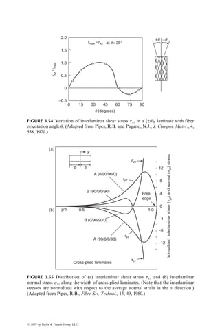
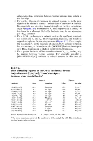
![(hj hj1)
2
6
6
6
6
6
6
6
6
6
4
3
7
7
7
7
7
7
7
7
7
5
[T
] ¼
1
2
P
N
j¼1
(
Q11)j(axx)j þ (
Q12)j(ayy)j þ (
Q16)j(axy)j](https://image.slidesharecdn.com/fiberreinforcedcompositesmaterialsmanufacturinganddesignp1-220510152925-9ef3de0d/85/Fiber_Reinforced_Composites_Materials_Manufacturing_and_Design_P-1-pdf-234-320.jpg)
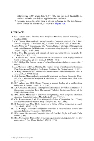
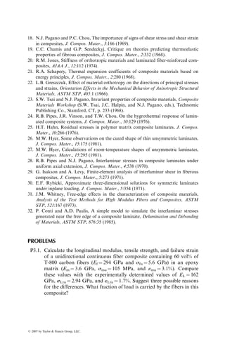
![h2
j h2
j1
2
6
6
6
6
6
6
6
6
6
4
3
7
7
7
7
7
7
7
7
7
5
(3:110)
Note that even if no external loads are applied, that is, if [N] ¼ [M] ¼ [0], there
may be midplane strains and curvatures due to thermal effects, which in turn
will create thermal stresses in various laminas. These stresses can be calculated
using midplane strains and curvatures due to thermal effects in Equation 3.106.
When a composite laminate is cooled from the curing temperature to room
temperature, significant curing (residual) stresses may develop owing to the
thermal mismatch of various laminas. In some cases, these curing stresses may
be sufficiently high to cause intralaminar cracks [25]. Therefore, it may be
prudent to consider them in the analysis of composite laminates.
For example, consider a [0=90]S laminate being cooled from the curing
temperature to room temperature. If the plies were not joined and could
contract freely, the 08 ply will contract much less in the x direction than the
908 ply, while the reverse is true in the y direction. Since the plies are joined and
must deform together, internal residual stresses are generated to maintain the
geometric compatibility between the plies. In [0=90]S laminate, residual stresses
ß 2007 by Taylor Francis Group, LLC.](https://image.slidesharecdn.com/fiberreinforcedcompositesmaterialsmanufacturinganddesignp1-220510152925-9ef3de0d/85/Fiber_Reinforced_Composites_Materials_Manufacturing_and_Design_P-1-pdf-237-320.jpg)
![are compressive in the fiber direction, but tensile in the transverse direction in
both 08 and 908 plies (see Example 3.16). Thus, when such a laminate is loaded
in tension in the x direction, residual tensile stress added to the applied tensile
stress can initiate transverse cracks in the 908 plies at relatively low loads.
Equations 3.108 and 3.109 are also useful for calculating the coefficients of
thermal expansion and the cured shapes of a laminate. This is demonstrated in
the following two examples.
EXAMPLE 3.14
Coefficients of thermal expansion for a balanced symmetric laminate
SOLUTION
For a balanced symmetric laminate, A16 ¼ A26 ¼ 0 and [B] ¼ [0]. In a thermal
experiment, [N] ¼ [M] ¼ [0]. Therefore, from Equation 3.108,
0
0
0
2
4
3
5 ¼
A11 A12 0
A12 A22 0
0 0 A66
2
4
3
5
«
xx
«
yy
g
xy
2
4
3
5
T1*
T2*
T3*
2
4
3
5DT,
which gives
A11«
xx þ A12«
yy ¼ T1
*DT,
A12«
xx þ A22«
yy ¼ T2
*DT,
and
A66g
xy ¼ T3
*DT:
From the first two of these equations, we calculate «xx
8 and «yy
8 as
«
xx ¼
A22T1
* A12T2
*
A11A22 A2
12
DT,
«
yy ¼
A11T2
* A12T1
*
A11A22 A2
12
DT:
Following the definitions of thermal expansion coefficients, we write
axx ¼
«
xx
DT
¼
A22T1
* A12T2
*
A11A22 A2
12
,
ayy ¼
«
yy
DT
¼
A11T2
* A12T1
*
A11A22 A2
12
,
axy ¼
g
xy
DT
¼
T3
*
A66
:
ß 2007 by Taylor Francis Group, LLC.](https://image.slidesharecdn.com/fiberreinforcedcompositesmaterialsmanufacturinganddesignp1-220510152925-9ef3de0d/85/Fiber_Reinforced_Composites_Materials_Manufacturing_and_Design_P-1-pdf-238-320.jpg)
![For a balanced symmetric laminate, elements in the [T**] matrix are zero. There-
fore, there will be no curvatures due to temperature variation. However, the same
is not true for unsymmetric laminates.
EXAMPLE 3.15
Determine the curvatures of a two-layer unsymmetric [0=90] laminate after it
is cooled from the curing temperature to the room temperature. The material is
T-300 carbon fiber in an epoxy matrix for which a11 ¼ 0.5 3 106
m=m per 8C
and a22 ¼ 12 3 106
m=m per 8C. Other material properties are the same as those
in Example 3.6. The thickness of each layer is t, and the temperature drop is DT.
SOLUTION
From Example 3.6, the stiffness matrices for the 08 and 908 layers are
[Q]0 ¼
134:03 2:29 0
2:29 8:82 0
0 0 3:254
2
6
4
3
7
5 109
N=m2
,
[Q]90 ¼
8:82 2:29 0
2:29 134:03 0
0 0 3:254
2
6
4
3
7
5 109
N=m2
:
Step 1: Determine the [A], [B], and [D] matrices for the laminate.
Referring to the figure (top), we note that h0 ¼ t, h1 ¼ 0, and h2 ¼ t. Following
Equations 3.90 through 3.92, the [A], [B], and [D] matrices for the [0=90] laminate
can be written.
[A] ¼
142:85 4:58 0
4:58 142:85 0
0 0 6:508
2
6
4
3
7
5 109
t N=m,
[B] ¼
62:605 0 0
0 62:605 0
0 0 0
2
6
4
3
7
5 109
t2
N,
[D] ¼
47:62 1:53 0
1:53 47:62 0
0 0 2:17
2
6
4
3
7
5 109
t3
N m:
Step 2: Determine the [T*] and [T**] matrices for the laminate.
The first element in the [T*] matrix is
T1
* ¼ [(
Q11)1(axx)1 þ (
Q12)1(ayy)1](0 þ t)
þ [(
Q11)2(axx)2 þ (
Q12)2(ayy)2](t 0):
ß 2007 by Taylor Francis Group, LLC.](https://image.slidesharecdn.com/fiberreinforcedcompositesmaterialsmanufacturinganddesignp1-220510152925-9ef3de0d/85/Fiber_Reinforced_Composites_Materials_Manufacturing_and_Design_P-1-pdf-239-320.jpg)
(106
)t
þ [(8:82)(12) þ (2:29)(0:5)](109
)(106
)t
¼ 65:16 103
t N=m
C:
Using appropriate expressions for other elements in [T*] and [T**], we obtain
[T*] ¼
65:16
65:16
0
2
6
4
3
7
5 103
t N=m
C,
[T**] ¼
72:12
72:12
0
2
6
4
3
7
5 103
t2
N=
C:
Step 3: Determine the laminate curvature matrix.
Substitution of [T*] and [T**] in Equations 3.108 and 3.109 gives
0
0
0
2
6
4
3
7
5 ¼ [A]
«
xx
«
yy
g
xy
2
6
4
3
7
5 þ [B]
kxx
kyy
kxy
2
6
4
3
7
5
65:16
65:16
0
2
6
4
3
7
5 103
tDT,
0
0
0
2
6
4
3
7
5 ¼ [B]
«
xx
«
yy
g
xy
2
6
4
3
7
5 þ [D]
kxx
kyy
kxy
2
6
4
3
7
5
72:12
72:12
0
2
6
4
3
7
5 103
t2
DT,
where [A], [B], and [D] are laminate stiffness matrices.
Eliminating the midplane strain matrix from the previous equations, we
obtain the following expression relating the laminate curvature matrix to tem-
perature variation DT:
[k] ¼ [C1][T*] þ [D1][T
],
ß 2007 by Taylor Francis Group, LLC.](https://image.slidesharecdn.com/fiberreinforcedcompositesmaterialsmanufacturinganddesignp1-220510152925-9ef3de0d/85/Fiber_Reinforced_Composites_Materials_Manufacturing_and_Design_P-1-pdf-240-320.jpg)
![where [C1] and [D1] are given in Equation 3.95.
In this example,
[C1] ¼
0:0218 0 0
0 0:0218 0
0 0 0
2
6
4
3
7
5109
t2 1
N
,
[D1] ¼
0:0497 0:0016 0
0:0016 0:0497 0
0 0 0:4608
2
6
4
3
7
5109
t3 1
N m
:
Therefore, solving for [k], we obtain
kxx ¼ kyy ¼ 5:119 106
t1
DT per m,
kxy ¼ 0:
From the expressions for kxx and kyy, we note that both curvatures decrease with
increasing layer thickness as well as decreasing temperature variation. Further-
more, since kyy ¼ kxx, the laminate will assume a saddle shape at room tempera-
ture, as shown in the figure ((b) on page 207).
Classical lamination theory, such as that used here, predicts the room tempera-
ture shapes of all unsymmetric laminates to be a saddle. However, Hyer [26,27] has
shown that both cylindrical and saddle shapes are possible, as shown in the figure ((c)
on page 207). The cured shape of the laminate depends on the thickness–width ratio
as well as the thickness–length ratio. Saddle shapes are obtained for thick laminates,
but depending on the relative values of length and width, two different cylindrical
shapes (with either kxx or kyy ¼ 0) are obtained for thin laminates in which the
thickness–length or thickness–width ratios are small. It should be noted that sym-
metric laminates do not curve (warp) on curing since [B] ¼ [0] as well as [T**]¼ [0].
EXAMPLE 3.16
Residual stresses generated because of cooling from high curing temperatures:
A [0=902]S laminate of AS-4 carbon fiber–epoxy is cured at temperature
Ti ¼ 1908C and slowly cooled down to room temperature, Tf ¼ 238C. Determine
the residual stresses generated in each layer because of cooling from the curing
temperature. Assume each layer in the laminate has a thickness t0.
Midplane
t0
(1) 0
(2) 90
(3) 90
(4) 90
(5) 90
(6) 0
+z
ß 2007 by Taylor Francis Group, LLC.](https://image.slidesharecdn.com/fiberreinforcedcompositesmaterialsmanufacturinganddesignp1-220510152925-9ef3de0d/85/Fiber_Reinforced_Composites_Materials_Manufacturing_and_Design_P-1-pdf-241-320.jpg)
![Following material properties are known:
E11 ¼ 142 GPa,
E22 ¼ 10:3 GPa,
n12 ¼ 0:27,
G12 ¼ 7:6 GPa,
a11 ¼ 1:8 106
per
C,
a22 ¼ 27 106
per
C:
SOLUTION
Step 1: Using Equation 3.80, determine stiffness matrices for the 08 and 908 layers.
[
Q]0 ¼
142:77 2:796 0
2:796 10:356 0
0 0 7:6
2
6
4
3
7
5 109
N=m2
,
[
Q]90 ¼
10:356 2:796 0
2:796 142:77 0
0 0 7:6
2
6
4
3
7
5 109
N=m2
:
Step 2: Determine the [A] matrix for the laminate.
Note that because of symmetry, [B] ¼ [0] and, since [k] ¼ [0], we need not deter-
mine the [D] matrix.
For a [0=902]S laminate, Amn ¼ 2t0 [(
Qmn)0 þ 2(
Qmn)90]. Therefore,
[A] ¼ 2t0
163:48 8:39 0
8:39 295:90 0
0 0 22:8
2
4
3
5 109
N=m:
Step 3: Determine the [T*] matrix for the laminate.
T1
* ¼ 2[{(
Q11)0(axx)0 þ (
Q12)0(ayy)0 þ 0}( 2t0 þ 3t0)
þ {(
Q11)90(axx)90 þ (
Q12)90(ayy)90 þ 0}( t0 þ 2t0)
þ {(
Q11)90(axx)90 þ (
Q12)90(ayy)90 þ 0}(0 þ t0)]:
Since (axx)0 ¼ (ayy)90 ¼ a11 ¼ 1.8 3 106
per 8C and (ayy)0 ¼ (axx)90 ¼ a22 ¼ 27 3
106
per 8C, we obtain
T1
* ¼ 735:32t0 103
N=m
C:
ß 2007 by Taylor Francis Group, LLC.](https://image.slidesharecdn.com/fiberreinforcedcompositesmaterialsmanufacturinganddesignp1-220510152925-9ef3de0d/85/Fiber_Reinforced_Composites_Materials_Manufacturing_and_Design_P-1-pdf-242-320.jpg)
![Similarly, T2
* ¼ 176.82 t0 3 103
N=m 8C and T3
* ¼ 0.
Therefore,
[T*] ¼
735:32t0
176:82t0
0
2
4
3
5 103
N=m
C:
Step 4: Using Equation 3.108, determine the midplane strains.
Since there are no external forces, [N] ¼ [0]. Since [B] ¼ [0], we can write Equation
3.108 as
[0] ¼ [A]
«
xx
«
yy
g
xy
2
4
3
5 þ [0]
T1
*
T2
*
T3
*
2
4
3
5DT,
where DT ¼ Tf Ti (which, in this case, has a negative value).
Solving for the strain components gives
«
xx
«
yy
g
xy
2
4
3
5 ¼
2:267
0:352
0
2
4
3
5 106
DT m=m:
Step 5: Determine strains in each layer.
Since [k] ¼ [0], strains in each layer are the same as the midplane strains.
Step 6: Determine the free thermal contraction strains in each layer.
«xxf
«yyf
gxyf
2
4
3
5
0
¼
1:8
27
0
2
4
3
5 106
DT m=m
and
«xxf
«yyf
gxyf
2
4
3
5
90
¼
27
1:8
0
2
4
3
5 106
DT m=m:
Step 7: Subtract free thermal contraction strains from strains determined in Step 5
to obtain residual strains in each layer.
«xxr
«yyr
gxyr
2
4
3
5
0
¼
(2:267 (1:8) 106
DT
(0:352 27) 106
DT
0
2
4
3
5 ¼
4:067
27:352
0
2
4
3
5 106
DT m=m
and
«xxr
«yyr
gxyr
2
4
3
5
90
¼
(2:267 27) 106
DT
(0:352 (1:8)) 106
DT
0
2
4
3
5 ¼
24:733
1:448
0
2
4
3
5 106
DT m=m:
ß 2007 by Taylor Francis Group, LLC.](https://image.slidesharecdn.com/fiberreinforcedcompositesmaterialsmanufacturinganddesignp1-220510152925-9ef3de0d/85/Fiber_Reinforced_Composites_Materials_Manufacturing_and_Design_P-1-pdf-243-320.jpg)
![Step 8: Calculate the residual stresses in each layer
sxxr
syyr
txyr
2
6
4
3
7
5
0
¼ [
Q]0
«xxr
«yyr
gxyr
2
6
4
3
7
5
0
¼
504:17
271:89
0
2
6
4
3
7
5 103
DT N=m2
and
sxxr
syyr
txyr
2
6
4
3
7
5
90
¼ [
Q]90
«xxr
«yyr
gxyr
2
6
4
3
7
5
90
¼
252:087
137:550
0
2
6
4
3
7
5 103
DT N=m2
:
Since, in this case, DT ¼ 238C 1908C ¼ 1678C, the residual stresses are as follows:
08 Layer 908 Layer
In the fiber direction 84.2 MPa 22.97 MPa
In the transverse direction 45.40 MPa 42.10 MPa
3.4 INTERLAMINAR STRESSES
Load transfer between adjacent layers in a fiber-reinforced laminate takes place
by means of interlaminar stresses, such as szz, txz, and tyz. To visualize the
mechanism of load transfer, let us consider a balanced symmetric [±45]S
laminate under uniaxial tensile load Nxx (Figure 3.52). Since A16 ¼ A26 ¼ 0
and [B] ¼ [0] for this laminate, the midplane strains are given by
«
xx ¼
A22
A11A22 A2
12
Nxx,
«
yy ¼
A12
A11A22 A2
12
Nxx,
g
xy ¼ 0:
The state of stress in the jth layer is
sxx
syy
txy
2
6
4
3
7
5
j
¼
Q11
Q12
Q16
Q12
Q22
Q26
Q16
Q26
Q66
2
6
4
3
7
5
j
«
xx
«
yy
0
2
6
4
3
7
5:
ß 2007 by Taylor Francis Group, LLC.](https://image.slidesharecdn.com/fiberreinforcedcompositesmaterialsmanufacturinganddesignp1-220510152925-9ef3de0d/85/Fiber_Reinforced_Composites_Materials_Manufacturing_and_Design_P-1-pdf-244-320.jpg)
![Thus, although the shear stress resultant Nxy on the laminate is zero, each layer
experiences an in-plane shear stress txy. Since there is no applied shear stress at
the laminate boundary, the in-plane shear stress must diminish from a finite
value in the laminate interior to zero at its free edges. The large shear stress
gradient at the ends of the laminate width is equilibrated by the development of
the interlaminar shear stress txz near the free edges, as shown in Figure 3.52.
Similar equilibrium arguments can be made to demonstrate the presence of tyz
and szz in other laminates.
The principal reason for the existence of interlaminar stresses is the mis-
match of Poisson’s ratios nxy and coefficients of mutual influence mx and my
between adjacent laminas. If the laminas were not bonded and could deform
freely, an axial loading in the x direction would create dissimilar transverse
strains «yy in various laminas because of the difference in their Poisson’s ratios.
However, in perfect bonding, transverse strains must be identical throughout
the laminate. The constraint against free transverse deformations produces
normal stress syy in each lamina and interlaminar shear stress tyz at the lamina
b
y
z
[45/−45/−45/45]
b = 8t0
Laminate
free
edge
Laminate
free
edge
Stress
components
normalized
with
respect
to
the
avg.
strain
in
the
x
direction
(10
6
)
b
x
2t0
txz
txz
txy
txy
sxx
sxx
Nxx
3.5
3.0
2.5
2.0
1.5
1.0
0.5
0
−1.0 −0.5 +1.0
+0.5
0
y/b
FIGURE 3.52 Interlaminar shear stress txz between the þ458 and 458 plies at the free
edges of a [±45]S laminate. (After Pipes, R.B. and Pagano, N.J., J. Compos. Mater., 4,
538, 1970.)
ß 2007 by Taylor Francis Group, LLC.](https://image.slidesharecdn.com/fiberreinforcedcompositesmaterialsmanufacturinganddesignp1-220510152925-9ef3de0d/85/Fiber_Reinforced_Composites_Materials_Manufacturing_and_Design_P-1-pdf-245-320.jpg)
![interfaces (Figure 3.53). Similarly, the difference in the coefficients of mutual
influence mx would create dissimilar shear strains gxy in various laminas only if
they were not bonded. For a bonded laminate, equal shear strains for all
laminas require the development of interlaminar shear stress tzx. Although
the force equilibrium in the y direction is maintained by the action of syy and
tyz, the force resultants associated with syy and tyz are not collinear.
The moment equilibrium about the x axis is satisfied by the action of the
interlaminar normal stress szz.
Interlaminar stresses szz, txz, and tyz are determined by numerical methods
(e.g., finite difference [28] or finite element methods [29,30]), which are beyond
the scope of this book. A few approximate methods have also been developed
[31,32]. For practical purposes, it may be sufficient to note the following.
1. Interlaminar stresses in laminated composites develop owing to mis-
match in the Poisson’s ratios and coefficients of mutual influence
between various layers. If there is no mismatch of these two engineering
properties, there are no interlaminar stresses regardless of the mismatch
in elastic and shear moduli.
2. Interlaminar stresses can be significantly high over a region equal to the
laminate thickness near the free edges of a laminate. The free edges may
be at the boundaries of a laminated plate, around a cutout or hole, or at
the ends of a laminated tube. As a result of high interlaminar stresses,
Top
free
surface
y
b
z
08
908
908
08
b b
Interface
between
08 and 908 laminas
szz
tyz
syy
t0
t0
t0
t0
t0
FIGURE 3.53 Source of interlaminar shear stress tyz and interlaminar normal stress szz
in a [0=90=90=0] laminate.
ß 2007 by Taylor Francis Group, LLC.](https://image.slidesharecdn.com/fiberreinforcedcompositesmaterialsmanufacturinganddesignp1-220510152925-9ef3de0d/85/Fiber_Reinforced_Composites_Materials_Manufacturing_and_Design_P-1-pdf-246-320.jpg)
![0
−0.5
0
0.5
1.0
1.5
2.0
15 30 45 60
q (degrees)
t
xz
/t
max
tmax =txz at q=35°
+q −q
75 90
FIGURE 3.54 Variation of interlaminar shear stress txz in a [±u]S laminate with fiber
orientation angle u. (Adapted from Pipes, R.B. and Pagano, N.J., J. Compos. Mater., 4,
538, 1970.)
y
b
A (0/90/90/0)
12
8
4
0
−4
−8
−12
B (0/90/90/0)
B (90/0/0/90)
A (90/0/0/90)
Cross-plied laminates
Free
edge
Normalized
interlaminar
shear
(t
yz
)
and
normal
(s
zz
)
stress
1.0
0.5
y/b
szz
szz
tyz
tyz
b
(a)
(b)
FIGURE 3.55 Distribution of (a) interlaminar shear stress tyz and (b) interlaminar
normal stress szz along the width of cross-plied laminates. (Note that the interlaminar
stresses are normalized with respect to the average normal strain in the x direction.)
(Adapted from Pipes, R.B., Fibre Sci. Technol., 13, 49, 1980.)
ß 2007 by Taylor Francis Group, LLC.](https://image.slidesharecdn.com/fiberreinforcedcompositesmaterialsmanufacturinganddesignp1-220510152925-9ef3de0d/85/Fiber_Reinforced_Composites_Materials_Manufacturing_and_Design_P-1-pdf-247-320.jpg)
![delamination (i.e., separation between various laminas) may initiate at
the free edges.
3. For an [u=u] angle-ply laminate in uniaxial tension, txz is the most
significant interlaminar stress at the interfaces of the u and –u laminas.
Its magnitude and direction depend strongly on the fiber orientation
angle u (Figure 3.54). Furthermore, txz has a higher value at the (u=u)
interfaces in a clustered [un=un]S laminate than in an alternating
[(u=u)n]S laminate.
4. For a [0=90] type laminate in uniaxial tension, the significant interlami-
nar stresses are szz and tyz. Their magnitude, locations, and directions
depend strongly on the stacking sequence (Figure 3.55). For example,
the maximum szz at the midplane of a [0=90=90=0] laminate is tensile,
but maximum szz at the midplane of a [90=0=0=90] laminate is compres-
sive. Thus, delamination is likely in the [0=90=90=0] laminate.
5. For a general laminate, different combinations of txz, tyz, and szz may
be present between various laminas. For example, consider a
[45=45=0=0=–45=45] laminate in uniaxial tension. In this case, all
TABLE 3.4
Effect of Stacking Sequence on the Critical Interlaminar Stresses
in Quasi-Isotropic [0=90=±45]S T-300 Carbon–Epoxy
Laminates under Uniaxial Tensiona
Max szz Max txz
Laminate Value Location Value Location
[90=45=0=45]S 6.8 Midplane 6.9 08=458
[0=45=90=45]S 6.2 908 layer 6.6 908=458
[45=90=0=45]S 6.6 908 layer 5.9 08=458
[45=90=45=0]S 6.9 908 layer 6.5 458=908
[45=0=90=45]S 7.6 908 layer 5.8 908=458
[45=0=45=90]S 10.4 Midplane 6.0 08=458
[90=0=45=45]S 8.2 458=458 9.0 458=458
[90=45=45=0]S 7.4 458=458 9.2 458=458
[0=90=45=45]S 7.6 458 layer 9.2 458=458
[0=45=45=90]S 10.0 Midplane 8.3 458=458
[45=45=90=0]S 9.0 08 layer 7.7 458=458
[45=45=0=90]S 10.9 Midplane 7.2 458=458
Source: Adapted from Herakovich, C.T., J. Compos. Mater., 15, 336, 1981.
a
The stress magnitudes are in ksi. To transform to MPa, multiply by 6.89. The (=) indicates
interface between adjacent layers.
ß 2007 by Taylor Francis Group, LLC.](https://image.slidesharecdn.com/fiberreinforcedcompositesmaterialsmanufacturinganddesignp1-220510152925-9ef3de0d/85/Fiber_Reinforced_Composites_Materials_Manufacturing_and_Design_P-1-pdf-248-320.jpg)
![three interlaminar stress components are present between the 45=45
layers as well as the 0=45 layers. However, the interlaminar shear stress
txz between adjacent 45=45 laminas is higher than that between adja-
cent 0=45 laminas. On the other hand, the interlaminar shear stress tyz
between 0=45 laminas is higher than that between 45=45 laminas.
However, the maximum szz occurs at the laminate midplane.
6. Stacking sequence has a strong influence on the nature, magnitude, and
location of interlaminar stresses. This is demonstrated in Table 3.4.
Note that laminates with interspersed ±458 layers (separated by 08 or
908 layers) have lower txz than those with adjacent ±458 layers, and,
therefore, are less likely to delaminate. Among the laminates with
0
−1.0
−0.8
−0.6
−0.4
−0.2
0
0.2
0.4
0.6
Normalized
interlaminar
shear
and
normal
stresses
Laminate
free
edge
Laminate
centerline
0.8
0.25 0.50
b
y
Carbon fiber–epoxy
(c)
Glass fiber–epoxy
Carbon fiber–epoxy
(b) tyz
txz
Glass fiber–epoxy
Carbon fiber–epoxy
(45/−45/0/0/−45/45)
(a) szz
Glass fiber–epoxy
y/b
0.75 1.00
b
FIGURE 3.56 Distribution of interlaminar stresses in [±45=0]S laminates with carbon
and glass fibers in an epoxy matrix. (Adapted from Pipes, R.B., Fibre Sci. Technol., 13,
49, 1980.)
ß 2007 by Taylor Francis Group, LLC.](https://image.slidesharecdn.com/fiberreinforcedcompositesmaterialsmanufacturinganddesignp1-220510152925-9ef3de0d/85/Fiber_Reinforced_Composites_Materials_Manufacturing_and_Design_P-1-pdf-249-320.jpg)
![interspersed ±458 layers, [90=45=0=45]S has the most favorable szz
under a uniaxial tensile load applied on the laminates.
7. Material properties also have a strong influence on the interlaminar
shear stresses of a laminate, as shown in Figure 3.56.
REFERENCES
1. G.S. Holister and C. Thomas, Fibre Reinforced Materials, Elsevier Publishing Co.,
London (1966).
2. C.C. Chamis, Micromechanics strength theories, Composite Materials, Vol. 5, Frac-
ture and Fatigue (L.J. Broutman, ed.), Academic Press, New York, p. 93 (1974).
3. A.N. Netravali, P. Schwartz, and S.L. Phoenix, Study of interfaces of high perform-
ance glass fibers and DGEBA-based epoxy resins using single-fiber-composite test,
Polym. Compos., 6:385 (1989).
4. H.L. Cox, The elasticity and strength of paper and other fibrous materials, Br.
J. Appl. Phys., 3:72 (1952).
5. J. Cook and J.E. Gordon, A mechanism for the control of crack propagation in all
brittle systems, Proc. R. Soc. Lond., A, 282:508 (1964).
6. D.C. Phillips, The fracture energy of carbon fibre reinforced glass, J. Mater. Sci., 7
(1972).
7. J.O. Outwater and M.C. Murphy, The fracture energy of unidirectional laminates,
Proc. 24th Annual Technical Conference, Society of the Plastics Industry (1969).
8. A. Kelly, Interface effects and the work of fracture of a fibrous composite, Proc. R.
Soc. Lond., A, 319:95 (1970).
9. G.A. Cooper, Micromechanics aspects of fracture and toughness, Composite Mater-
ials, Vol. 5, Fracture and Fatigue (L.J. Broutman, ed.), Academic Press, New York,
p. 415 (1974).
10. D.F. Adams and D.R. Doner, Transverse normal loading of a unidirectional
composite, J. Compos. Mater., 1:152 (1967).
11. L.B. Greszczuk, Theoretical and experimental studies on properties and behavior of
filamentary composites, Proc. 21st Annual Technical Conference, Society of the
Plastics Industry (1966).
12. B.W. Rosen, Mechanics of composite strengthening, Fiber Composite Materials,
American Society for Metals, Metals Park, OH, p. 37 (1965).
13. C.R. Schultheisz and A.M. Waas, Compressive failure of composites, Part I: Testing
and micromechanical theories, Prog. Aerospace Sci., 32:1 (1996).
14. B. Budiansky and N.A. Fleck, Compressive failure of fibre composites, J. Mech.
Phys. Solids., 41:183 (1993).
15. T.A. Collings, Transverse compressive behavior of unidirectional carbon fibre
reinforced plastics, Composites, 5:108 (1974).
16. R.M. Jones, Mechanics of Composite Materials, 2nd Ed., Taylor Francis, Phila-
delphia (1999).
17. R.M. Christensen, The numbers of elastic properties and failure parameters for fiber
composites, J. Eng. Mater. Technol., 120:110 (1998).
ß 2007 by Taylor Francis Group, LLC.](https://image.slidesharecdn.com/fiberreinforcedcompositesmaterialsmanufacturinganddesignp1-220510152925-9ef3de0d/85/Fiber_Reinforced_Composites_Materials_Manufacturing_and_Design_P-1-pdf-250-320.jpg)
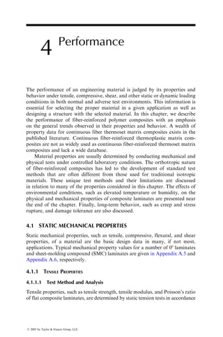
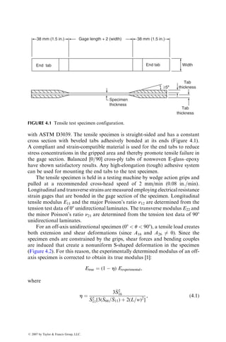
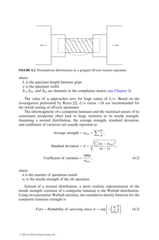
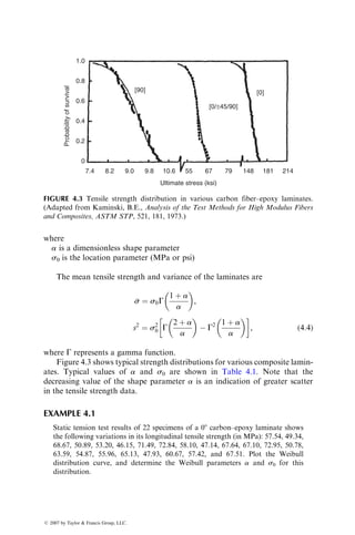
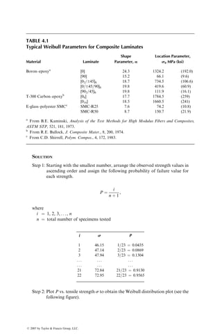
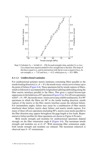
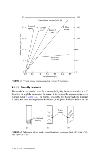
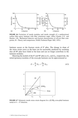
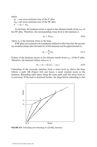
![9 3 106
and 100 3 106
per 8C, respectively. For the same compos-
ite, the major Poisson’s ratio is 0.32. The matrix properties are Em ¼ 2.8
GPa, nm ¼ 0.38, and am ¼ 60 3 106
per 8C. Using these values, esti-
mate (a) the Poisson’s ratio of the fiber, (b) coefficients of thermal
expansion of the fiber in longitudinal and radial directions, and (c)
the fiber volume fraction at which the composite has a zero CTE.
P3.31. A 1 m long thin-walled composite tube has a mean diameter of 25 mm
and its wall thickness is 2 mm. It contains 60 vol% E-glass fibers in a
vinyl ester matrix. Determine the change in length and diameter of the
tube if the temperature is increased by 508C. The matrix properties are
Em ¼ 3.5 GPa, nm ¼ 0.35, am ¼ 70 3 106
per 8C.
P3.32. An E-glass fiber–epoxy laminate has the following construction:
[0=30= 30=45= 45=90= 45=45= 30=30=0]:
The following are known: vf ¼ 0.60, Ef ¼ 10 3 106
psi, Em ¼ 0.34 3 106
psi, nf ¼ 0.2, nm ¼ 0.35, af ¼ 5 3 106
per 8C, and am ¼ 60 3 106
per 8C.
Determine the coefficients of thermal expansion in the x and y directions
for each lamina.
P3.33. Consider a unidirectional continuous fiber lamina. Applying s11, s22,
and t12 separately, show that the engineering elastic constants E11, E22,
n12, n21, and G12 can be expressed in terms of the elements in the lamina
stiffness matrix as
E11 ¼ Q11
Q2
12
Q22
,
E22 ¼ Q22
Q2
12
Q11
,
n12 ¼
Q12
Q22
,
n21 ¼
Q12
Q11
,
G12 ¼ Q66:
P3.34. A T-300 carbon fiber–epoxy lamina (vf ¼ 0.60) with a fiber orientation
angle of 458 is subjected to a biaxial stress state of sxx ¼ 100 MPa and
syy ¼ 50 MPa. Determine (a) the strains in the xy directions, (b) the
strains in the 1–2 directions, and (c) the stresses in the 1–2 directions.
Use the material property data of Example 3.6.
ß 2007 by Taylor Francis Group, LLC.](https://image.slidesharecdn.com/fiberreinforcedcompositesmaterialsmanufacturinganddesignp1-220510152925-9ef3de0d/85/Fiber_Reinforced_Composites_Materials_Manufacturing_and_Design_P-1-pdf-260-320.jpg)
![P3.35. Plot and compare the coefficients of mutual influence as functions of
fiber orientation angle u in T-300 carbon fiber–epoxy laminas contain-
ing fibers at the þu and u orientations. For what fiber orientation
angle u do the coefficients of mutual influence have the maximum
values? Use the material property data of Example 3.6.
P3.36. The elastic constants of a 08 unidirectional carbon fiber-reinforced
PEEK lamina are E11 ¼ 132.2 GPa, E22 ¼ 9.2 GPa, G12 ¼ 4.90 GPa,
and n12 ¼ 0.35. Write the compliance and stiffness matrices for the
same material if the fiber orientation angle is (a) 308, (b) 308, (c) 608,
and (d) 908.
P3.37. A T-300 carbon fiber–epoxy lamina (vf ¼ 0.6) is subjected to a uniaxial
normal stress sxx. Compare the strains in the xy directions as well as
in the 1–2 directions for u ¼ 08, þ458, 458, and 908. Use the material
property data of Example 3.6 and Problem P3.35.
P3.38. Compare the stiffness matrices of three-layered [0=60=60],
[60=0=60], and [60=60=60] laminates. Which of these laminates
can be considered quasi-isotropic, and why? Assume that each layer
has the same thickness t0.
P3.39. Compare the stiffness matrices of two-layered, three-layered, and four-
layered angle-ply laminates containing alternating u and u laminas.
Assume that each layer has the same thickness t0.
P3.40. Show that the extensional stiffness matrices for quasi-isotropic [0=
±60]S, [±60=0]S, and [60=0=60]S laminates are identical, while their
bending stiffness matrices are different.
P3.41. The modulus of a [0m=90n] laminate can be calculated using the follow-
ing ‘‘averaging’’ equation.
Exx ¼
m
m þ n
E11 þ
n
m þ n
E22:
Suppose a [0=90=0]3S laminate is constructed using continuous T-300
fibers in an epoxy matrix. Verify that the modulus of the laminate
calculated by the averaging equation is the same as calculated by the
lamination theory. Use the material properties given in Example 3.6.
P3.42. The [A] matrix for a boron fiber–epoxy [±45]S laminate of thickness h is
ß 2007 by Taylor Francis Group, LLC.](https://image.slidesharecdn.com/fiberreinforcedcompositesmaterialsmanufacturinganddesignp1-220510152925-9ef3de0d/85/Fiber_Reinforced_Composites_Materials_Manufacturing_and_Design_P-1-pdf-261-320.jpg)
![[A] ¼
0:99h 0:68h 0
0:68h 0:99h 0
0 0 0:72h
2
4
3
5 107
lb=in:
1. Calculate the engineering elastic constants for the laminate
2. Calculate the strains in the þ458 and 458 laminas owing to average
laminate stresses Nxx=h ¼ Nyy=h ¼ p and Nxy=h ¼ 0. Assume that
each lamina has a thickness of h=4
P3.43. The elastic properties of unidirectional carbon fiber–epoxy lamina are
E11 ¼ 181.3 GPa, E22 ¼ 10.27 GPa, G12 ¼ 7.17 GPa, and n12 ¼ 0.28.
Compare the engineering elastic constants of the [±45=0]S and
[±45=0=90]S laminates manufactured from this carbon fiber–epoxy
material.
P3.44. Show that the shear modulus of a thin [±45]nS plate is given by
Gxy ¼
1
4
E11 þ E22 2n12E22
1 n12n21
:
P3.45. Show that the elements in the bending stiffness matrix of [0=60=60]S
and [0=90=45=45]S laminates are given by
Dij ¼
h3
12
(
Qij)60 þ 7(
Qij)60 þ 19(
Qij)0
27
and
Dij ¼
h3
12
(
Qij)45 þ 7(
Qij)45 þ 19(
Qij)90 þ 37(
Qij)0
64
,
respectively. Here, h represents the laminate thickness.
P3.46. A torsional moment Mxy applied to a symmetric laminated plate creates
a bending curvature as well as a twisting curvature. Find an expression
for the additional bending moment Mxx that must be applied to the
plate to create a pure twisting curvature kxy.
P3.47. An ARALL-4 laminate contains three layers of 2024-T8 aluminum
alloy sheet (each 0.3 mm thick) and two layers of 08 unidirectional
Kevlar 49-epoxy in an alternate sequence, [A1=0K=A1=0K=A1]. Elastic
properties of the aluminum alloy are E ¼ 73 GPa and n ¼ 0.32, whereas
ß 2007 by Taylor Francis Group, LLC.](https://image.slidesharecdn.com/fiberreinforcedcompositesmaterialsmanufacturinganddesignp1-220510152925-9ef3de0d/85/Fiber_Reinforced_Composites_Materials_Manufacturing_and_Design_P-1-pdf-262-320.jpg)
![those for the Kevlar layers are E11 ¼ 56.2 GPa, E22 ¼ 4.55 GPa,
n12 ¼ 0.456, and G12 ¼ 1.85 GPa. The nominal thickness of the laminate
is 1.3 mm. Calculate the elastic properties of the ARALL-4 laminate.
P3.48. Using the basic ply level properties of Example 3.6, determine the
stresses in each layer of a [±45]32S laminate subjected to Nxx ¼ 0.1
N=mm. The ply thickness is 0.013 mm.
P3.49. Using the material properties in Example 3.16, determine the residual
thermal stresses in each lamina of (i) a [902=0]S and (ii) a [0=90=0]S
laminate. Both laminates are slowly cooled down from a curing tem-
perature of 1908C to 238C.
P3.50. The following thermomechanical properties are known for a carbon
fiber–epoxy composite: E11 ¼ 145 GPa, E22 ¼ 9 GPa, G12 ¼ 4.5 GPa,
n12 ¼ 0.246, a11 ¼ 0.25 3 106
per 8C, and a22 ¼ 34.1 3 106
per 8C.
Determine the coefficients of thermal expansion of a [45=45]S lamin-
ate of this material.
P3.51. Using the ply level thermomechanical properties given in Problem 3.49,
determine the coefficients of thermal expansion of a [0=45=45=90]S
laminate of this material.
P3.52. An approximate expression for the maximum interlaminar shear stress
txz in a [u=u]nS class of laminates* is
Max txz ¼
1
2n
A22
Q16 A12
Q26
A11A22 A2
12
Nxx
h
,
where Nxx=h is the average tensile stress on the laminate in the x
direction.
Using this expression, compare the maximum interlaminar shear
stress txz in [15=15]8S and [45=45]8S T-300 carbon–epoxy laminates.
Use Example 3.6 for the basic material property data.
P3.53. Following is an approximate expression* for the maximum interlami-
nar normal stress, szz, at an interface position z from the midplane of a
symmetric [0=90]S type laminate:
* J.M. Whitney, I.M. Daniel, and R.B. Pipes, Experimental Mechanics of Fiber Reinforced Com-
posite Materials, Society for Experimental Mechanics, Brookfield Center, CT (1984).
ß 2007 by Taylor Francis Group, LLC.](https://image.slidesharecdn.com/fiberreinforcedcompositesmaterialsmanufacturinganddesignp1-220510152925-9ef3de0d/85/Fiber_Reinforced_Composites_Materials_Manufacturing_and_Design_P-1-pdf-263-320.jpg)
![Max szz(z) ¼
90
sxx
7Ah
X
j
A22
Q12
j
A12
Q22
j
h i
tj(hj z),
where
sxx ¼ applied normal stress in the x direction
A ¼ A11A22 A12
2
h ¼ laminate thickness
hj ¼ distance from the midplane of the laminate to the midplane of
the jth lamina
tj ¼ thickness of the jth lamina
and the summation extends over all the laminas above the interface
position z. This equation is valid for thin laminas in which the variation
of in-plane stresses is assumed to be negligible over the thickness of each
lamina.
Using this approximate expression, compare the maximum inter-
laminar normal stresses at the midplanes of [0=90=90=0] and
[90=0=0=90] laminates.
ß 2007 by Taylor Francis Group, LLC.](https://image.slidesharecdn.com/fiberreinforcedcompositesmaterialsmanufacturinganddesignp1-220510152925-9ef3de0d/85/Fiber_Reinforced_Composites_Materials_Manufacturing_and_Design_P-1-pdf-264-320.jpg)
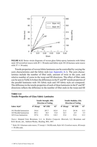
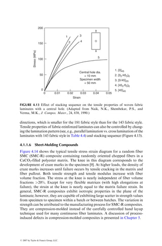
![with ASTM D3039. The tensile specimen is straight-sided and has a constant
cross section with beveled tabs adhesively bonded at its ends (Figure 4.1).
A compliant and strain-compatible material is used for the end tabs to reduce
stress concentrations in the gripped area and thereby promote tensile failure in
the gage section. Balanced [0=90] cross-ply tabs of nonwoven E-glass–epoxy
have shown satisfactory results. Any high-elongation (tough) adhesive system
can be used for mounting the end tabs to the test specimen.
The tensile specimen is held in a testing machine by wedge action grips and
pulled at a recommended cross-head speed of 2 mm=min (0.08 in.=min).
Longitudinal and transverse strains are measured employing electrical resistance
strain gages that are bonded in the gage section of the specimen. Longitudinal
tensile modulus E11 and the major Poisson’s ratio n12 are determined from the
tension test data of 08 unidirectional laminates. The transverse modulus E22 and
the minor Poisson’s ratio n21 are determined from the tension test data of 908
unidirectional laminates.
For an off-axis unidirectional specimen (08 u 908), a tensile load creates
both extension and shear deformations (since A16 and A26 6¼ 0). Since the
specimen ends are constrained by the grips, shear forces and bending couples
are induced that create a nonuniform S-shaped deformation in the specimen
(Figure 4.2). For this reason, the experimentally determined modulus of an off-
axis specimen is corrected to obtain its true modulus [1]:
Etrue ¼ (1 h) Eexperimental,
where
h ¼
3
S2
16
S2
11[3(
S66=
S11) þ 2(L=w)2
]
, (4:1)
≥58
Specimen
thickness
Tab
thickness
Tab
thickness
Width
End tab
38 mm (1.5 in.)
38 mm (1.5 in.) Gage length + 2 (width)
End tab
FIGURE 4.1 Tensile test specimen configuration.
ß 2007 by Taylor Francis Group, LLC.](https://image.slidesharecdn.com/fiberreinforcedcompositesmaterialsmanufacturinganddesignp1-220510152925-9ef3de0d/85/Fiber_Reinforced_Composites_Materials_Manufacturing_and_Design_P-1-pdf-267-320.jpg)
![where
L is the specimen length between grips
w is the specimen width
S11,
S16, and
S66 are elements in the compliance matrix (see Chapter 3)
The value of h approaches zero for large values of L=w. Based on the
investigation performed by Rizzo [2], L=w ratios 10 are recommended for
the tensile testing of off-axis specimens.
The inhomogeneity of a composite laminate and the statistical nature of its
constituent properties often lead to large variation in its tensile strength.
Assuming a normal distribution, the average strength, standard deviation,
and coefficient of variation are usually reported as
Average strength ¼ save ¼
X si
n
,
Standard deviation ¼ d ¼
ffiffiffiffiffiffiffiffiffiffiffiffiffiffiffiffiffiffiffiffiffiffiffiffiffiffiffiffiffiffi
P
si save
ð Þ2
(n 1)
s
,
Coefficient of variation ¼
100d
save
, (4:2)
where
n is the number of specimens tested
si is the tensile strength of the ith specimen
Instead of a normal distribution, a more realistic representation of the
tensile strength variation of a composite laminate is the Weibull distribution.
Using two-parameter Weibull statistics, the cumulative density function for the
composite laminate strength is
F(s) ¼ Probability of surviving stress s ¼ exp
s
s0
a
, (4:3)
FIGURE 4.2 Nonuniform deformation in a gripped off-axis tension specimen.
ß 2007 by Taylor Francis Group, LLC.](https://image.slidesharecdn.com/fiberreinforcedcompositesmaterialsmanufacturinganddesignp1-220510152925-9ef3de0d/85/Fiber_Reinforced_Composites_Materials_Manufacturing_and_Design_P-1-pdf-268-320.jpg)
![where
a is a dimensionless shape parameter
s0 is the location parameter (MPa or psi)
The mean tensile strength and variance of the laminates are
s ¼ s0G
1 þ a
a
,
s2
¼ s2
0 G
2 þ a
a
G2 1 þ a
a
, (4:4)
where G represents a gamma function.
Figure 4.3 shows typical strength distributions for various composite lamin-
ates. Typical values of a and s0 are shown in Table 4.1. Note that the
decreasing value of the shape parameter a is an indication of greater scatter
in the tensile strength data.
EXAMPLE 4.1
Static tension test results of 22 specimens of a 08 carbon–epoxy laminate shows
the following variations in its longitudinal tensile strength (in MPa): 57.54, 49.34,
68.67, 50.89, 53.20, 46.15, 71.49, 72.84, 58.10, 47.14, 67.64, 67.10, 72.95, 50.78,
63.59, 54.87, 55.96, 65.13, 47.93, 60.67, 57.42, and 67.51. Plot the Weibull
distribution curve, and determine the Weibull parameters a and s0 for this
distribution.
1.0
0.8
[90] [0]
[0/±45/90]
0.6
0.4
0.2
0
7.4 8.2 9.0 9.8 10.6 55 67
Ultimate stress (ksi)
Probability
of
survival
79 148 181 214
FIGURE 4.3 Tensile strength distribution in various carbon fiber–epoxy laminates.
(Adapted from Kaminski, B.E., Analysis of the Test Methods for High Modulus Fibers
and Composites, ASTM STP, 521, 181, 1973.)
ß 2007 by Taylor Francis Group, LLC.](https://image.slidesharecdn.com/fiberreinforcedcompositesmaterialsmanufacturinganddesignp1-220510152925-9ef3de0d/85/Fiber_Reinforced_Composites_Materials_Manufacturing_and_Design_P-1-pdf-269-320.jpg)
![SOLUTION
Step 1: Starting with the smallest number, arrange the observed strength values in
ascending order and assign the following probability of failure value for
each strength.
P ¼
i
n þ 1
,
where
i ¼ 1, 2, 3, . . . , n
n ¼ total number of specimens tested
i s P
1 46.15 1=23 ¼ 0.0435
2 47.14 2=23 ¼ 0.0869
3 47.94 3=23 ¼ 0.1304
. . . . . . . . .
. . . . . . . . .
21 72.84 21=23 ¼ 0.9130
22 72.95 22=23 ¼ 0.9565
Step 2: Plot P vs. tensile strength s to obtain the Weibull distribution plot (see the
following figure).
TABLE 4.1
Typical Weibull Parameters for Composite Laminates
Material Laminate
Shape
Parameter, a
Location Parameter,
s0 MPa (ksi)
Boron–epoxya
[0] 24.3 1324.2 (192.0)
[90] 15.2 66.1 (9.6)
[02=±45]S 18.7 734.5 (106.6)
[0=±45=90]S 19.8 419.6 (60.9)
[902=45]S 19.8 111.9 (16.1)
T-300 Carbon–epoxyb
[08] 17.7 1784.5 (259)
[016] 18.5 1660.5 (241)
E-glass–polyester SMCc
SMC-R25 7.6 74.2 (10.8)
SMC-R50 8.7 150.7 (21.9)
a
From B.E. Kaminski, Analysis of the Test Methods for High Modulus Fibers and Composites,
ASTM STP, 521, 181, 1973.
b
From R.E. Bullock, J. Composite Mater., 8, 200, 1974.
c
From C.D. Shirrell, Polym. Compos., 4, 172, 1983.
ß 2007 by Taylor Francis Group, LLC.](https://image.slidesharecdn.com/fiberreinforcedcompositesmaterialsmanufacturinganddesignp1-220510152925-9ef3de0d/85/Fiber_Reinforced_Composites_Materials_Manufacturing_and_Design_P-1-pdf-270-320.jpg)
![1.0
0.8
0.6
0.4
Probability
of
failure
Probability
of
survival
Tensile strength (MPa)
0.2
0
30 40 50 60 70 80
0
0.2
0.4
0.6
0.8
1.0
Step 3: CalculateYP ¼ ln{ln[1=(1 P)]} for eachstrengthvalue,andplotYP vs.lns.
Use a linear least-squares method to fit a straight line to the data. The slope of
this line is equal to a, and its intersection with the ln s axis is equal to ln s0. In
our example, a ¼ 7.62 and lns0 ¼ 4.13, which gives s0 ¼ 62.1 MPa.
4.1.1.2 Unidirectional Laminates
For unidirectional polymer matrix laminates containing fibers parallel to the
tensile loading direction (i.e., u ¼ 08), the tensile stress–strain curve is linear up to
the point of failure (Figure 4.4). These specimens fail by tensile rupture of fibers,
which is followed or accompanied by longitudinal splitting (debonding along the
fiber–matrix interface) parallel to the fibers. This gives a typical broom-type
appearanceinthe failedarea of08specimens (Figure 4.5a).Foroff-axisspecimens
with08 u 908,thetensilestress–strain curvesmayexhibitnonlinearity. For908
specimens in which the fibers are 908 to the tensile loading direction, tensile
rupture of the matrix or the fiber–matrix interface causes the ultimate failure.
For intermediate angles, failure may occur by a combination of fiber–matrix
interfacial shear failure, matrix shear failure, and matrix tensile rupture. For
many of these off-axis specimens (including 908), matrix craze marks parallel to
the fiber direction may appear throughout the gage length at low loads. Repre-
sentative failure profiles for these specimens are shown in Figure 4.5b and c.
Both tensile strength and modulus for unidirectional specimens depend
strongly on the fiber orientation angle u (Figure 4.6). The maximum tensile
strength and modulus are at u ¼ 08. With increasing fiber orientation angle,
both tensile strength and modulus are reduced. The maximum reduction is
observed near u ¼ 08 orientations.
ß 2007 by Taylor Francis Group, LLC.](https://image.slidesharecdn.com/fiberreinforcedcompositesmaterialsmanufacturinganddesignp1-220510152925-9ef3de0d/85/Fiber_Reinforced_Composites_Materials_Manufacturing_and_Design_P-1-pdf-271-320.jpg)
![4.1.1.3 Cross-Ply Laminates
The tensile stress–strain curve for a cross-ply [0=90]S laminate tested at u ¼ 08
direction is slightly nonlinear; however, it is commonly approximated as a
bilinear curve (Figure 4.7). The point at which the two linear sections intersect
is called the knee and represents the failure of 908 plies. Ultimate failure of the
1,725
1,380
1,035
690
345
0
25
Fiber volume fraction (vf) = 0.6
Boron−
epoxy HT Carbon−
epoxy Kevlar 49−
epoxy
S-Glass−
epoxy
Aluminum
(7075-T6)
Tensile strain (%)
0.0 0.5 1.0 1.5 2.0 2.5 3.0
20
15
10
Tensile
stress
(10,000
psi)
5
0
FIGURE 4.4 Tensile stress–strain curves for various 08 laminates.
Longitudinal
splitting
Craze
marks
(a) (b) (c)
FIGURE 4.5 Schematic failure modes in unidirectional laminates: (a) u ¼ 08, (b) u ¼ 908,
and (c) 0 u 908.
ß 2007 by Taylor Francis Group, LLC.](https://image.slidesharecdn.com/fiberreinforcedcompositesmaterialsmanufacturinganddesignp1-220510152925-9ef3de0d/85/Fiber_Reinforced_Composites_Materials_Manufacturing_and_Design_P-1-pdf-272-320.jpg)
![laminate occurs at the fracture strain of 08 plies. The change in slope of
the stress–strain curve at the knee can be reasonably predicted by assuming
that all 908 plies have failed at the knee and can no longer contribute to the
laminate modulus.
Denoting the moduli of the 08 and 908 plies as E11 and E22, respectively, the
initial (primary) modulus of the cross-ply laminate can be approximated as
E ¼
A0
A
E11 þ
A90
A
E22, (4:5)
80
60
40
Strength
(ksi)
20
0
40
30
20
10
0
0
0 30 60 90
100
200
300
90
60
q (degrees)
q (degrees)
30
0
(b)
(a)
0
10
20
Strength
(MPa)
Modulus
(Msi)
Modulus
(GPa)
30
40
50
s
q
s
60
FIGURE 4.6 Variations of tensile modulus and tensile strength of a unidirectional
carbon fiber–epoxy laminate with fiber orientation angle. (After Chamis, C.C. and
Sinclair, J.H., Mechanical behavior and fracture characteristics of off-axis fiber com-
posites, II—Theory and comparisons, NASA Technical Paper 1082, 1978.)
[90]
[0]
s
sF
sk
[0/90]S
Knee
E
eTt eLt e
ES
FIGURE 4.7 Schematic tensile stress–strain diagram for a [0=90]S cross-plied laminate
tested at u ¼ 08 direction.
ß 2007 by Taylor Francis Group, LLC.](https://image.slidesharecdn.com/fiberreinforcedcompositesmaterialsmanufacturinganddesignp1-220510152925-9ef3de0d/85/Fiber_Reinforced_Composites_Materials_Manufacturing_and_Design_P-1-pdf-273-320.jpg)
![where
A0 ¼ net cross-sectional area of the 08 plies
A90 ¼ net cross-sectional area of the 908 plies
A ¼ A0 þ A90
At the knee, the laminate strain is equal to the ultimate tensile strain «TU of
the 908 plies. Therefore, the corresponding stress level in the laminate is
sk ¼ E«TU, (4:6)
where sk is the laminate stress at the knee.
If 908 plies are assumed to be completely ineffective after they fail, the second-
ary modulus (slope after the knee) Es of the laminate can be approximated as
Es ¼
A0
A
E11: (4:7)
Failure of the laminate occurs at the ultimate tensile strain «LU of the 08 plies.
Therefore, the laminate failure stress sF is
sF ¼ sk þ Es «LU «TU
ð Þ: (4:8)
Unloading of the cross-ply laminate from a stress level sL above the knee
follows a path AB (Figure 4.8) and leaves a small residual strain in the
laminate. Reloading takes place along the same path until the stress level sL
is recovered. If the load is increased further, the slope before unloading is also
A
sL
sk
C
B D
Stress
Strain
FIGURE 4.8 Unloading and reloading of a [0=90]S laminate.
ß 2007 by Taylor Francis Group, LLC.](https://image.slidesharecdn.com/fiberreinforcedcompositesmaterialsmanufacturinganddesignp1-220510152925-9ef3de0d/85/Fiber_Reinforced_Composites_Materials_Manufacturing_and_Design_P-1-pdf-274-320.jpg)
![recovered. Unloading from a higher stress level follows a path CD, which has a
smaller slope than AB. The difference in slope between the two unloading paths
AB and CD is evidence that the 908 plies fail in a progressive manner. Neglect-
ing the small residual strains after unloading, Hahn and Tsai [6] predicted the
elastic modulus ED of the damaged laminate as
ED ¼
E
1 þ [(AE=A0E11) 1](1 sk=sL)
: (4:9)
4.1.1.4 Multidirectional Laminates
Tensile stress–strain curves for laminates containing different fiber orientations
in different laminas are in general nonlinear. A few examples are shown in
Figure 4.9. For the purposes of analysis, these curves are approximated by a
number of linear portions that have different slopes. When these linear portions
are extended, a number of knees, similar to that observed in a cross-ply
laminate, can be identified. The first knee in these diagrams is called the first
ply failure (FPF) point. Many laminates retain a significant load-carrying
capacity beyond the FPF point, but for some laminates with high notch
sensitivity, failure occurs just after FPF (Table 4.2). Furthermore, cracks
appearing at the FPF may increase the possibility of environmental damage
(such as moisture pickup) as well as fatigue failure. For all these reasons, the
FPF point has special importance in many laminate designs.
Angle-ply laminates containing [±u] layups exhibit two kinds of stress–
strain nonlinearity (Figure 4.10). At values of u closer to 08, a stiffening effect
140
120
80
40
0
0 2 4
Strain (10−6
)
[0/±45]S
[0/±45/90]S
[±45/90]S
Stress
(MPa)
Stress
(ksi)
6
1104
828
552
276
0
FIGURE 4.9 Typical tensile stress–strain diagrams for multidirectional laminates.
ß 2007 by Taylor Francis Group, LLC.](https://image.slidesharecdn.com/fiberreinforcedcompositesmaterialsmanufacturinganddesignp1-220510152925-9ef3de0d/85/Fiber_Reinforced_Composites_Materials_Manufacturing_and_Design_P-1-pdf-275-320.jpg)
![TABLE 4.2
Tensile Strengths and First-Ply Failure (FPF) Stresses in High-Strength
Carbon–Epoxy Symmetric Laminatesa
UTS, MPa (ksi)
Estimated FPF Stress,
MPa (ksi)
Tensile
Modulus,
GPa (Msi)
Initial
Tensile
Strain (%)
Laminate Resin 1 Resin 2 Resin 1 Resin 2
[0]S 1378 (200) 1378 (200) — — 151.6 (22) 0.3
[90]S 41.3 (6) 82.7 (12) — — 8.96 (1.3) 0.5–0.9
[±45]S 137.8 (20) 89.6 (13) 89.6 (13) 89.6 (13) 17.2 (2.5) 1.5–4.5
[0=90]S 447.8 (65) 757.9 (110) 413.4 (60) 689 (100) 82.7 (12) 0.5–0.9
[02=±45]S 599.4 (87) 689 (110) 592.5 (86) 689 (100) 82.7 (12) 0.8–0.9
[0=±60]S 461.6 (67) 551.2 (80) 323.8 (47) 378.9 (55) 62 (9) 0.8–0.9
[0=90=±45]S 385.8 (56) 413.4 (60) 275.6 (40) 413.4 (60) 55.1 (8) 0.8–0.9
Source: Adapted from Freeman, W.T. and Kuebeler, G.C., Composite Materials: Testing and
Design (Third Conference), ASTM STP, 546, 435, 1974.
a
Resin 2 is more flexible than resin 1 and has a higher strain-to-failure.
AS carbon−epoxy
[±15]S
[±30]S
[±45]S
[±60]S
Stress
(100
MPa)
Stress
(10,000
psi)
[90]
0
0
2
4
6
8
4 8 12
Strain (10−3
)
16 20
0
2.9
5.8
8.7
11.6
FIGURE 4.10 Typical tensile stress–strain diagrams for angle-ply laminates. (Adapted
from Lagace, P.A., AIAA J., 23, 1583, 1985.)
ß 2007 by Taylor Francis Group, LLC.](https://image.slidesharecdn.com/fiberreinforcedcompositesmaterialsmanufacturinganddesignp1-220510152925-9ef3de0d/85/Fiber_Reinforced_Composites_Materials_Manufacturing_and_Design_P-1-pdf-276-320.jpg)
![is observed so that the modulus increases with increasing load. At larger values
of u, a softening effect is observed so that the modulus decreases with the
increasing load [7]. The stiffening effect is attributed to the longitudinal tensile
stresses in various plies, whereas the softening effect is attributed to the
shear stresses. Stiffening laminates do not exhibit residual strain on unloading.
Softening laminates, on the other hand, exhibit a residual strain on unloading
and a hysteresis loop on reloading. However, the slope of the stress–strain
curve during reloading does not change from the slope of the original stress–
strain curve.
The tensile failure mode and the tensile strength of a multidirectional
laminate containing laminas of different fiber orientations depend strongly
on the lamina stacking sequence. An example of the stacking sequence effect
is observed in the development of cracks in [0=±45=90]S and [0=90=±45]S
laminates (Figure 4.11). In both laminates, intralaminar transverse cracks
(parallel to fibers) appear in the 908 plies. However, they are arrested at the
0
0
0
+45
−45
90
+45
+45
−45
−45
90
90
90
−45
+45
0
Delamination
Transverse cracks
Transverse cracks
(a)
(b)
FIGURE 4.11 Damage development in (a) [0=±45=90]S and (b) [0=90=±45]S laminates
subjected to static tension loads in the 08 direction.
ß 2007 by Taylor Francis Group, LLC.](https://image.slidesharecdn.com/fiberreinforcedcompositesmaterialsmanufacturinganddesignp1-220510152925-9ef3de0d/85/Fiber_Reinforced_Composites_Materials_Manufacturing_and_Design_P-1-pdf-277-320.jpg)
![lamina interfaces and do not immediately propagate into the adjacent plies. The
number of transverse cracks in the 908 plies increases until uniformly spaced
cracks are formed throughout the specimen length [8]; however, these trans-
verse cracks are more closely spaced in [0=90=±45]S laminates than [0=±45=90]S
laminates. Increasing the tensile load also creates a few intralaminar cracks
parallel to the fiber directions in both 458 and þ458 plies. Apart from these
intralaminar crack patterns, subsequent failure modes in these two apparently
similar laminates are distinctly different. In [0=±45=90]S laminates, longitudinal
interlaminar cracks grow between the 908 plies, which join together to form
continuous edge delaminations with occasional jogging into the 90=45 inter-
faces. With increasing load, the edge delamination extends toward the center of
the specimen; however, the specimen fails by the rupture of 08 fibers before the
entire width is delaminated. In contrast to the [0=±45=90]S laminate, there is no
edge delamination in the [0=90=±45]S laminate; instead, transverse cracks
appear in both þ458 and 458 plies before the laminate failure. The difference
in edge delamination behavior between the [0=±45=90]S and [0=90=±45]S lamin-
ates can be explained in terms of the interlaminar normal stress szz, which is
tensile in the former and compressive in the latter.
Table 4.3 presents the tensile test data and failure modes observed in several
multidirectional carbon fiber–epoxy laminates. If the laminate contains 908
plies, failure begins with transverse microcracks appearing in these plies. With
increasing stress level, the number of these transverse microcracks increases
until a saturation number, called the characteristic damage state (CDS),
is reached. Other types of damages that may follow transverse microcracking
are delamination, longitudinal cracking, and fiber failure.
4.1.1.5 Woven Fabric Laminates
The principal advantage of using woven fabric laminates is that they provide
properties that are more balanced in the 08 and 908 directions than unidirec-
tional laminates. Although multilayered laminates can also be designed to
produce balanced properties, the fabrication (layup) time for woven fabric
laminates is less than that of a multilayered laminate. However, the tensile
strength and modulus of a woven fabric laminate are, in general, lower than
those of multilayered laminates. The principal reason for their lower tensile
properties is the presence of fiber undulation in woven fabrics as the fiber yarns
in the fill direction cross over and under the fiber yarns in the warp direction to
create an interlocked structure. Under tensile loading, these crimped fibers tend
to straighten out, which creates high stresses in the matrix. As a result, micro-
cracks are formed in the matrix at relatively low loads. This is also evidenced by
the appearance of one or more knees in the stress–strain diagrams of woven
fabric laminates (Figure 4.12). Another factor to consider is that the fibers in
woven fabrics are subjected to additional mechanical handling during the
weaving process, which tends to reduce their tensile strength.
ß 2007 by Taylor Francis Group, LLC.](https://image.slidesharecdn.com/fiberreinforcedcompositesmaterialsmanufacturinganddesignp1-220510152925-9ef3de0d/85/Fiber_Reinforced_Composites_Materials_Manufacturing_and_Design_P-1-pdf-278-320.jpg)
![TABLE 4.3
Tensile Test Data and Failure Modes of Several Symmetric Carbon Fiber-Reinforced Epoxy Laminates
Laminate Type
Secant Modulus
at Low
Strain, GPa
Failure Stress,
MPa
Failure
Strain
Transverse
Ply Strain
Cracking Failure Modes (in Sequence)
[04=90]S
[04=902]S
[04=904]S
[04=908]S
122
109
93
72
1620
1340
1230
930
0.0116
0.011
0.0114
0.0115
0.0065
0.004
0.0035
0.003
Small transverse ply cracks in 908 plies, transverse cracks growing
in number as well as in length up to 08 plies, delamination at 0=90
interfaces, 08 ply failure
[±45]S
[þ452=452]S
[þ453=453]S
[þ45=452=45]S
[(þ45=45)2]S
17.3
19
14
18.2
17
126
135
89
152
125
0.017
0.0117
0.01
0.016
0.014
—
—
—
—
—
Edge crack formation, edge cracks growing across the width parallel
to fiber direction, delamination at the þ45=45 interfaces, single
or multiple ply failure
[±45=902=02]S
[±45=02=902]S
[02=±45=902]S
[02=902=±45]S
64.2
61.2
56.4
59.1
690
630
640
670
0.014
0.014
0.012
0.012
0.0028
0.0022
0.0016
0.0035
Transverse microcracks in 908 plies, longitudinal or angled cracks
in 908 plies in the first three laminates, a few edge cracks in 458 plies,
delamination (45=90, 0=90, ±45, and 45=0 interfaces in ascending
order of threshold strain), longitudinal ply failure
Source: Adapted from Harrison, R.P. and Bader, M.G., Fibre Sci. Technol., 18, 163, 1983.
ß
2007
by
Taylor
Francis
Group,
LLC.](https://image.slidesharecdn.com/fiberreinforcedcompositesmaterialsmanufacturinganddesignp1-220510152925-9ef3de0d/85/Fiber_Reinforced_Composites_Materials_Manufacturing_and_Design_P-1-pdf-279-320.jpg)
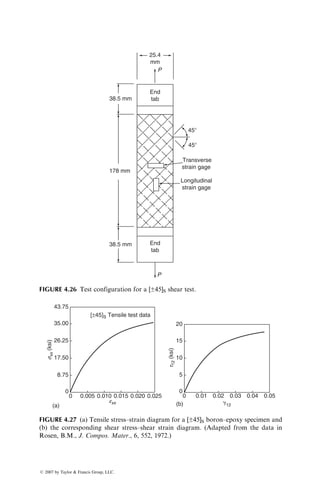
![directions, which is smaller for the 181 fabric style than for the 143 fabric style.
Tensile properties of fabric-reinforced laminates can also be controlled by chang-
ing the lamination pattern (see, e.g., parallel lamination vs. cross lamination of the
laminates with 143 fabric style in Table 4.4) and stacking sequence (Figure 4.13).
4.1.1.6 Sheet-Molding Compounds
Figure 4.14 shows the typical tensile stress–strain diagram for a random fiber
SMC (SMC-R) composite containing randomly oriented chopped fibers in a
CaCO3-filled polyester matrix. The knee in this diagram corresponds to the
development of craze marks in the specimen [9]. At higher loads, the density of
craze marks increases until failure occurs by tensile cracking in the matrix and
fiber pullout. Both tensile strength and tensile modulus increase with fiber
volume fraction. The stress at the knee is nearly independent of fiber volume
fractions 20%. Except for very flexible matrices (with high elongations at
failure), the strain at the knee is nearly equal to the matrix failure strain. In
general, SMC-R composites exhibit isotropic properties in the plane of the
laminate; however, they are capable of exhibiting large scatter in strength values
from specimen to specimen within a batch or between batches. The variation in
strength can be attributed to the manufacturing process for SMC-R composites.
They are compression-molded instead of the carefully controlled hand layup
technique used for many continuous fiber laminates. A discussion of process-
induced defects in compression-molded composites is presented in Chapter 5.
1
2
3
4
5
1. [0]4S
2. [02/452]S
3. [0/45]2S
4. [452/02]S
5. [45]4S
Central hole dia.
= 10 mm
Specimen width
= 50 mm
200
150
100
Stress
(MPa)
Strain
50
0
0 0.01 0.02 0.03 0.04 0.05
FIGURE 4.13 Effect of stacking sequence on the tensile properties of woven fabric
laminates with a central hole. (Adapted from Naik, N.K., Shembekar, P.S., and
Verma, M.K., J. Compos. Mater., 24, 838, 1990.)
ß 2007 by Taylor Francis Group, LLC.](https://image.slidesharecdn.com/fiberreinforcedcompositesmaterialsmanufacturinganddesignp1-220510152925-9ef3de0d/85/Fiber_Reinforced_Composites_Materials_Manufacturing_and_Design_P-1-pdf-281-320.jpg)
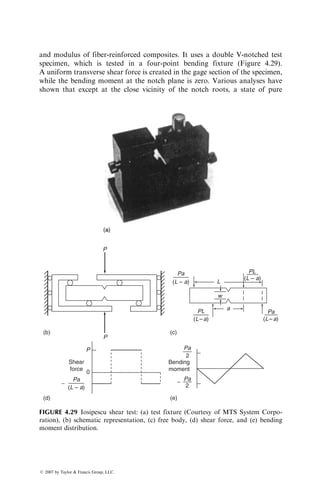
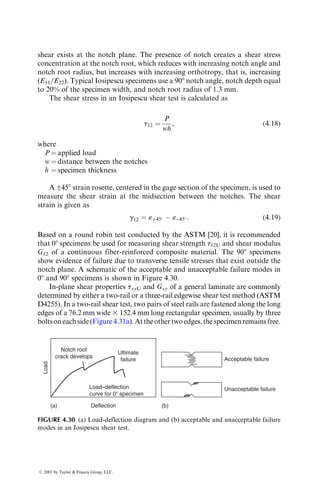
![in the hybrid begin to fail is either greater than or equal to the ultimate tensile
strain of the LE fibers. Furthermore, instead of failing catastrophically, the LE
fibers now fail in a controlled manner, giving rise to a step or smooth inflection
in the tensile stress–strain diagram. During this period, multiple cracks are
observed in the LE fiber layers [10].
The ultimate strength of interply hybrid laminates is lower than the tensile
strengths of either the LE or the HE fiber composites (Figure 4.18). Note that
4
3
2
1
0
0 1
Strain (%)
Tensile
load
(lbs)
2 3
FIGURE 4.17 Tensile stress–strain diagram for a GY-70 carbon=S glass–epoxy
interply hybrid laminate. (After Aveston, J. and Kelly, A., Phil. Trans. R. Soc. Lond.,
A, 294, 519, 1980.)
200 40
30
20
10
0
150
100
50
Strength
Modulus
0
0 20 40
Relative carbon fiber content (vol%)
Tensile
modulus
(Msi)
Tensile
strength
(ksi)
60 80 100
FIGURE 4.18 Variations of tensile strength and modulus of a carbon=glass–epoxy
interply hybrid laminate with carbon fiber content. (After Kalnin, L.E., Composite
Materials: Testing and Design (Second Conference), ASTM STP, 497, 551, 1972.)
ß 2007 by Taylor Francis Group, LLC.](https://image.slidesharecdn.com/fiberreinforcedcompositesmaterialsmanufacturinganddesignp1-220510152925-9ef3de0d/85/Fiber_Reinforced_Composites_Materials_Manufacturing_and_Design_P-1-pdf-284-320.jpg)
![the ultimate strain of interply hybrid laminates is also lower than that of the
HE fiber composite. The tensile modulus of the interply hybrid laminate falls
between the tensile modulus values of the LE and HE fiber composites. Thus, in
comparison to the LE fiber composite, the advantage of an interply hybrid
laminate subjected to tensile loading is the enhanced strain-to-failure. However,
this enhancement of strain, referred to as the hybrid effect, is achieved at the
sacrifice of tensile strength and tensile modulus.
The strength variation of hybrid laminates as a function of LE fiber content
was explained by Manders and Bader [11]. Their explanation is demonstrated
in Figure 4.19, where points A and D represent the tensile strengths of an
all-HE fiber composite and an all-LE fiber composite, respectively. If each type
of fiber is assumed to have its unique failure strain, the first failure event in
the interply hybrid composite will occur when the average tensile strain in it
exceeds the failure strain of the LE fibers. The line BD represents the stress
in the interply hybrid composite at which failure of the LE fibers occurs. The
line AE represents the stress in the interply hybrid composite assuming that
the LE fibers carry no load. Thus, if the LE fiber content is less than vc, the
ultimate tensile strength of the interply hybrid laminate is controlled by the HE
fibers. Even though the LE fibers have failed at stress levels given by the line
BC, the HE fibers continue to sustain increasing load up to the level given by
the line AC. For LE fiber contents greater than vc, the HE fibers fail almost
immediately after the failure of the LE fibers. Thus, the line ACD represents the
tensile strength of the interply hybrid laminate. For comparison, the rule of
mixture prediction, given by the line AD, is also shown in Figure 4.19.
A
B
0 0.5
vc
Volume fraction of low-elongation (LE) fibers
1.0
Tensile
strength
C
Rule of mixture
D
E
FIGURE 4.19 Model for tensile strength variation in interply hybrid laminates.
ß 2007 by Taylor Francis Group, LLC.](https://image.slidesharecdn.com/fiberreinforcedcompositesmaterialsmanufacturinganddesignp1-220510152925-9ef3de0d/85/Fiber_Reinforced_Composites_Materials_Manufacturing_and_Design_P-1-pdf-285-320.jpg)
![4.1.2 COMPRESSIVE PROPERTIES
Compressive properties of thin composite laminates are difficult to measure
owing to sidewise buckling of specimens. A number of test methods and
specimen designs have been developed to overcome the buckling problem
[12]. Three of these test methods are described as follows.
Celanese test: This was the first ASTM standard test developed for testing
fiber-reinforced composites in compression; however, because of its several
deficiencies, it is no longer a standard test. It employs a straight-sided specimen
with tabs bonded at its ends and 108 tapered collet-type grips that fit into
sleeves with a matching inner taper (Figure 4.20). An outer cylindrical shell is
used for ease of assembly and alignment. As the compressive load is applied at
Specimen
3.99 mm
(a)
Collet
grip
Tapered
sleeve
Cylindrical
shell
63.5
mm
diameter
63.5 mm
12.7 mm
63.5 mm
10⬚
FIGURE 4.20 (a) Celanese test specimen and fixture for compression testing.
(continued)
ß 2007 by Taylor Francis Group, LLC.](https://image.slidesharecdn.com/fiberreinforcedcompositesmaterialsmanufacturinganddesignp1-220510152925-9ef3de0d/85/Fiber_Reinforced_Composites_Materials_Manufacturing_and_Design_P-1-pdf-286-320.jpg)
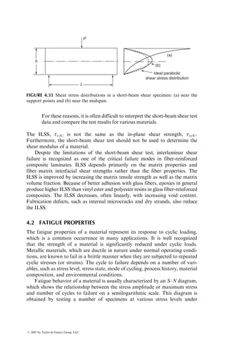
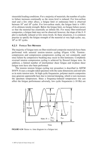
![3. The longitudinal compressive strength of a 08 laminate depends on the fiber
type, fiber volume fraction, matrix yield strength, fiber length–diameter
ratio, fiber straightness, fiber alignment as well as fiber–matrix interfacial
shear strength. The effects of some of these variables on the compressive
properties of unidirectional fiber-reinforced polyester composites have
been studied by Piggott and Harris and are described in Ref. [4].
End cap
Composite
specimens
Aluminum
honeycomb
FIGURE 4.22 Sandwich edgewise compression testing specimen.
TABLE 4.5
Compressive Properties of Carbon and Boron Fiber-Reinforced
Epoxy Composites
Carbon–Epoxy Boron–Epoxy
Laminate
Strength, MPa
(ksi)
Modulus, GPa
(Msi)
Strength, MPa
(ksi)
Modulus, GPa
(Msi)
[0] 1219.5 (177) 110.9 (16.1) 2101.4 (305) 215.6 (31.3)
[±15] 799.2 (116) 95.8 (13.9) 943.9 (137) 162.9 (23.65)
[±45] 259.7 (37.7) 15.6 (2.27) 235.6 (34.2) 17.4 (2.53)
[90] 194.3 (28.2) 13.1 (1.91) 211.5 (30.7) 20.5 (2.98)
[0=90] 778.6 (113) 60.6 (8.79) 1412.4 (205) 118.3 (17.17)
[0=±45=90] 642.8 (93.3) 46.4 (6.74) 1054.2 (153) 79.0 (11.47)
Source: Adapted from Weller, T., Experimental studies of graphite=epoxy and boron=epoxy angle
ply laminates in compression, NASA Report No. NASA-CR-145233, September 1977.
ß 2007 by Taylor Francis Group, LLC.](https://image.slidesharecdn.com/fiberreinforcedcompositesmaterialsmanufacturinganddesignp1-220510152925-9ef3de0d/85/Fiber_Reinforced_Composites_Materials_Manufacturing_and_Design_P-1-pdf-289-320.jpg)
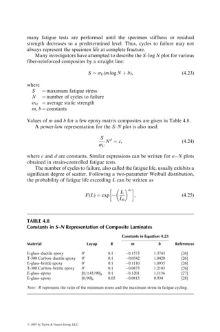
![EF ¼
mL3
4bh3
, (4:11)
where m is the initial slope of the load–deflection curve.
Three-point flexural tests have received wide acceptance in the composite
material industry because the specimen preparation and fixtures are very
simple. However, the following limitations of three-point flexural tests should
be recognized.
1. The maximum fiber stress may not always occur at the outermost layer
in a composite laminate. An example is shown in Figure 4.24. Thus,
Equation 4.10 gives only an apparent strength value. For more accurate
values, lamination theory should be employed.
2. In the three-point bending mode, both normal stress sxx and shear stress
txz are present throughout the beam span. If contributions from both
stresses are taken into account, the total deflection at the midspan of the
beam is
D ¼
PL3
4Ebh3
|fflffl{zfflffl}
normal
þ
3PL
10Gbh
|fflfflffl{zfflfflffl}
shear
¼
PL3
4Ebh3
1 þ
12
10
E
G
h
L
2
#
: (4:12)
90
0
90
90
90
90
90
90
0
90
(a) (b)
0
90
0
0
0
0
0
0
90
0
FIGURE 4.24 Normal stress (sxx) distributions in various layers of (a) [90=0=
(90)6=0=90] and (b) [0=90=(0)6=90=0] laminates under flexural loading.
ß 2007 by Taylor Francis Group, LLC.](https://image.slidesharecdn.com/fiberreinforcedcompositesmaterialsmanufacturinganddesignp1-220510152925-9ef3de0d/85/Fiber_Reinforced_Composites_Materials_Manufacturing_and_Design_P-1-pdf-291-320.jpg)
![This equation shows that the shear deflection can be quite significant in
a composite laminate, since the E=G ratio for fiber-reinforced compos-
ites is often quite large. The shear deflection can be reduced employing a
high span–thickness (L=h) ratio for the beam. Based on data of Zweben
et al. [13], L=h ratios of 60:1 are recommended for the determination of
flexural modulus.
3. Owing to large deflection at high L=h ratios, significant end forces are
developed at the supports. This in turn affects the flexural stresses in a
beam. Unless a lower L=h ratio, say 16:1, is used, Equation 4.10 must be
corrected for these end forces in the following way:
max ¼
3PmaxL
2bh2
1 þ 6
D
L
2
4
h
L
D
L
#
, (4:13)
where D is given by Equation 4.12.
4. Although the flexural strength value is based on the maximum tensile
stress in the outer fiber, it does not reflect the true tensile strength of the
material. The discrepancy arises owing to the difference in stress dis-
tributions in flexural and tensile loadings. Flexural loads create a non-
uniform stress distribution along the length, but a tensile load creates a
uniform stress distribution. Using a two-parameter Weibull distribution
for both tensile strength and flexural strength variations, the ratio of
the median flexural strength to the median tensile strength can be
written as
sUF
sUT
¼ 2(1 þ a)2 VT
VF
1=a
, (4:14)
where
a ¼ shape parameter in the Weibull distribution function (assumed
to be equal in both tests)
VT ¼ volume of material stressed in a tension test
VF ¼ volume of material stressed in a three-point flexural test
Assuming VT ¼ VF and using typical values of a ¼ 15 and 25 for 08
E-glass–epoxy and 08 carbon–epoxy laminates, respectively [12], Equation 4.14
shows that
sUF ¼ 1.52sUT for 08 E-glass–epoxy laminates
sUF ¼ 1.33sUT for 08 carbon–epoxy laminates
ß 2007 by Taylor Francis Group, LLC.](https://image.slidesharecdn.com/fiberreinforcedcompositesmaterialsmanufacturinganddesignp1-220510152925-9ef3de0d/85/Fiber_Reinforced_Composites_Materials_Manufacturing_and_Design_P-1-pdf-292-320.jpg)
![Thus, the three-point flexural strength of a composite laminate can be signifi-
cantly higher than its tensile strength. The experimental data presented by
Bullock [14] as well as Whitney and Knight [15] verify this observation.
Figure 4.25 shows the flexural load-deflection diagrams for four unidirec-
tional 08 laminates. The materials of construction are an ultrahigh-modulus
carbon (GY-70), a high-strength carbon (T-300), Kevlar 49, and E-glass fiber-
reinforced epoxies. The difference in slope in their load–deflection diagrams
reflects the difference in their respective fiber modulus. The GY-70 laminate
exhibits a brittle behavior, but other laminates exhibit a progressive failure
mode consisting of fiber failure, debonding (splitting), and delamination. The
Kevlar 49 laminate has a highly nonlinear load–deflection curve due to com-
pressive yielding. Fiber microbuckling damages are observed on the compres-
sion side of both E-glass and T-300 laminates. Since high contact stresses just
under the loading point create such damage, it is recommended that a large
loading nose radius be used.
The flexural modulus is a critical function of the lamina stacking sequence
(Table 4.6), and therefore, it does not always correlate with the tensile modulus,
which is less dependent on the stacking sequence. In angle-ply laminates,
a bending moment creates both bending and twisting curvatures. Twisting
curvature causes the opposite corners of a flexural specimen to lift off its
supports. This also influences the measured flexural modulus. The twisting
curvature is reduced with an increasing length–width (L=b) ratio and a decreasing
degree of orthotropy (i.e., decreasing E11=E22).
800
600
400
200
0
0 0.05 0.10 0.15 0.20 0.25
Deflection (in.)
Kevlar 49–epoxy
E-glass–epoxy
T-300 Carbon–epoxy
GY-70 Carbon−
epoxy
Load
(lbs)
Three-point flexural test with L/h=11–16
unidirectional (0⬚) laminates
FIGURE 4.25 Load–deflection diagrams for various 08 unidirectional laminates in
three-point flexural tests.
ß 2007 by Taylor Francis Group, LLC.](https://image.slidesharecdn.com/fiberreinforcedcompositesmaterialsmanufacturinganddesignp1-220510152925-9ef3de0d/85/Fiber_Reinforced_Composites_Materials_Manufacturing_and_Design_P-1-pdf-293-320.jpg)
![4.1.4 IN-PLANE SHEAR PROPERTIES
A variety of test methods [16,17] have been used for measuring in-plane shear
properties, such as the shear modulus G12 and the ultimate shear strength t12U
of unidirectional fiber-reinforced composites. Three common in-plane shear
test methods for measuring these two properties are described as follows.
±45 Shear test: The ±45 shear test (ASTM D3518) involves uniaxial tensile
testing of a [þ45=45]nS symmetric laminate (Figure 4.26). The specimen
dimensions, preparation, and test procedure are the same as those described
in the tension test method ASTM D3039. A diagram of the shear stress t12 vs.
the shear strain g12 is plotted using the following equations:
t12 ¼
1
2
sxx,
g12 ¼ «xx «yy, (4:15)
where sxx, «xx, and «yy represent tensile stress, longitudinal strain, and trans-
verse strain, respectively, in the [±45]nS tensile specimen. A typical tensile stress–
tensile strain response of a [±45]S boron–epoxy laminate and the corresponding
shear stress–shear strain diagram are shown in Figure 4.27.
108 Off-axis test: The 108 off-axis test [18] involves uniaxial tensile testing of
a unidirectional laminate with fibers oriented at 108 from the tensile loading
direction (Figure 4.28). The shear stress t12 is calculated from the tensile stress
sxx using the following expression:
t12 ¼
1
2
sxx sin 2uju¼10 ¼ 0:171sxx: (4:16)
TABLE 4.6
Tensile and Flexural Properties of Quasi-Isotropic Laminates
Tension Test Flexural Testa
Laminate
Configurationb
Strength,
MPa (ksi)
Modulus,
GPa (Msi)
Strength,
MPa (ksi)
Modulus,
GPa (Msi)
[0=±45=90]S 506.4 (73.5) 48.23 (7) 1219.5 (177) 68.9 (10)
[90=±45=0]S 405.8 (58.9) 45.47 (6.6) 141.2 (20.5) 18.6 (2.7)
[45=0=45=90]S 460.9 (66.9) 46.85 (6.8) 263.9 (38.3) 47.54 (6.9)
Source: Adapted from Whitney, J.M., Browning, C.E., and Mair, A., Composite Materials: Testing
and Design (Third Conference), ASTM STP, 546, 30, 1974.
a
Four-point flexural test with L=h ¼ 32 and L=b ¼ 4.8.
b
Material: AS carbon fiber–epoxy composite, vf ¼ 0.6, eight plies.
ß 2007 by Taylor Francis Group, LLC.](https://image.slidesharecdn.com/fiberreinforcedcompositesmaterialsmanufacturinganddesignp1-220510152925-9ef3de0d/85/Fiber_Reinforced_Composites_Materials_Manufacturing_and_Design_P-1-pdf-294-320.jpg)
![25.4
mm
45⬚
45⬚
38.5 mm
38.5 mm
End
tab
End
tab
P
178 mm
Transverse
strain gage
Longitudinal
strain gage
P
FIGURE 4.26 Test configuration for a [±45]S shear test.
43.75
35.00
[±45]S Tensile test data
26.25
17.50
s
xx
(ksi)
t
12
(ksi)
exx
8.75
0
0 0 0.01 0.02 0.03
␥12
0.04 0.05
(a) (b)
20
15
10
5
0
0.005 0.010 0.015 0.020 0.025
FIGURE 4.27 (a) Tensile stress–strain diagram for a [±45]S boron–epoxy specimen and
(b) the corresponding shear stress–shear strain diagram. (Adapted from the data in
Rosen, B.M., J. Compos. Mater., 6, 552, 1972.)
ß 2007 by Taylor Francis Group, LLC.](https://image.slidesharecdn.com/fiberreinforcedcompositesmaterialsmanufacturinganddesignp1-220510152925-9ef3de0d/85/Fiber_Reinforced_Composites_Materials_Manufacturing_and_Design_P-1-pdf-295-320.jpg)
![Calculation of the shear strain g12 requires measurements of three normal
strains using either a rectangular strain gage rosette or a 608 D-strain gage
rosette. If a rectangular strain gage rosette is used (Figure 4.28), the expression
for shear strain g12 is
g12 ¼ 0:5977«g1 1:8794«g2 þ 1:2817«g3, (4:17)
where «g1, «g2, and «g3 are normal strains in gage 1, 2, and 3, respectively.
Iosipescu shear test: The Iosipescu shear test (ASTM D5379) was originally
developed by Nicolai Iosipescu for shear testing of isotropic materials and was
later adopted by Walrath and Adams [19] for determining the shear strength
P
45°
45°
10⬚
10°
1
2
x
y
2
3
Strain
gage
rosette
P
45⬚
45⬚
2
3
1
FIGURE 4.28 Test configuration for a 108 off-axis shear test.
ß 2007 by Taylor Francis Group, LLC.](https://image.slidesharecdn.com/fiberreinforcedcompositesmaterialsmanufacturinganddesignp1-220510152925-9ef3de0d/85/Fiber_Reinforced_Composites_Materials_Manufacturing_and_Design_P-1-pdf-296-320.jpg)
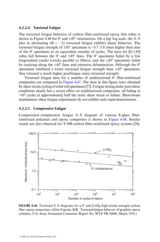
![shear exists at the notch plane. The presence of notch creates a shear stress
concentration at the notch root, which reduces with increasing notch angle and
notch root radius, but increases with increasing orthotropy, that is, increasing
(E11=E22). Typical Iosipescu specimens use a 908 notch angle, notch depth equal
to 20% of the specimen width, and notch root radius of 1.3 mm.
The shear stress in an Iosipescu shear test is calculated as
t12 ¼
P
wh
, (4:18)
where
P ¼ applied load
w ¼ distance between the notches
h ¼ specimen thickness
A ±458 strain rosette, centered in the gage section of the specimen, is used to
measure the shear strain at the midsection between the notches. The shear
strain is given as
g12 ¼ «þ45 «45 : (4:19)
Based on a round robin test conducted by the ASTM [20], it is recommended
that 08 specimens be used for measuring shear strength t12U and shear modulus
G12 of a continuous fiber-reinforced composite material. The 908 specimens
show evidence of failure due to transverse tensile stresses that exist outside the
notch plane. A schematic of the acceptable and unacceptable failure modes in
08 and 908 specimens is shown in Figure 4.30.
In-plane shear properties txyU and Gxy of a general laminate are commonly
determined by either a two-rail or a three-rail edgewise shear test method (ASTM
D4255). In a two-rail shear test, two pairs of steel rails are fastened along the long
edges of a 76.2 mm wide 3 152.4 mm long rectangular specimen, usually by three
boltsoneachside(Figure4.31a).Attheothertwoedges,thespecimenremainsfree.
Load
Notch root
crack develops
Ultimate
failure
Load–deflection
curve for 0⬚ specimen
Deflection
Acceptable failure
Unacceptable failure
(b)
(a)
FIGURE 4.30 (a) Load-deflection diagram and (b) acceptable and unacceptable failure
modes in an Iosipescu shear test.
ß 2007 by Taylor Francis Group, LLC.](https://image.slidesharecdn.com/fiberreinforcedcompositesmaterialsmanufacturinganddesignp1-220510152925-9ef3de0d/85/Fiber_Reinforced_Composites_Materials_Manufacturing_and_Design_P-1-pdf-298-320.jpg)
![A tensileloadappliedtotherailstendstodisplaceone railrelativetotheother, thus
inducing an in-plane shear load on the test laminate. In a three-rail shear test, three
pairs of steel rails are fastened to a 136 mm wide 3 152 mm long rectangular
specimen, two along its long edges, and one along its centerline (Figure 4.31b).
A compressive load applied at the center rail creates an in-plane shear load in
the specimen. The shear stress txy is calculated from the applied load P as
Two-rail: txy ¼
P
Lh
,
Three-rail: txy ¼
P
2Lh
, (4:20)
where
L is the specimen length
h is the specimen thickness
The shear strain gxy is determined using a strain gage mounted in the center
of the test section at 458 to the specimen’s longitudinal axis. The shear strain gxy
is calculated from the normal strain in the 458 direction:
gxy ¼ 2«45 : (4:21)
In order to assure a uniform shear stress field at a short distance away from the
free edges of a rail shear specimen [21], the length–width ratio must be greater
than 10:1. A low effective Poisson’s ratio for the laminate is also desirable, since
Rail
P
Rail
Specimen
(a)
P
P
Specimen
Side rail
Side rail
Center rail
(b)
P
FIGURE 4.31 Test configuration for (a) two-rail and (b) three-rail shear tests.
ß 2007 by Taylor Francis Group, LLC.](https://image.slidesharecdn.com/fiberreinforcedcompositesmaterialsmanufacturinganddesignp1-220510152925-9ef3de0d/85/Fiber_Reinforced_Composites_Materials_Manufacturing_and_Design_P-1-pdf-299-320.jpg)
![the shear stress distribution in laminates of a high Poisson’s ratio is irregular
across the width. For shear properties of unidirectional laminates, either 08 or 908
orientation (fibers parallel or perpendicular to the rails) can be used. However,
normal stress concentration near the free edges is transverse to the fibers in a 08
orientation and parallel to the fibers in the 908 orientation. Since normal stresses
may cause premature failure in the 08 laminate, it is recommended that a 908
laminate be used for determining t12U and G12 [22].
Although the results from various in-plane shear tests do not always
correlate, several general conclusions can be made:
1. The shear stress–strain response for fiber-reinforced composite mater-
ials is nonlinear.
2. Even though 08 laminates have superior tensile strength and modulus,
their shear properties are poor.
The shear strength and modulus depend on the fiber orientation angle and
laminate configuration. The highest shear modulus is obtained with [±45]S
symmetric laminates (Table 4.7). The addition of 08 layers reduces both the
shear modulus and the shear strength of [±45]S laminates.
4.1.5 INTERLAMINAR SHEAR STRENGTH
Interlaminar shear strength (ILSS) refers to the shear strength parallel to the
plane of lamination. It is measured in a short-beam shear test in accordance
with ASTM D2344. A flexural specimen of small span–depth (L=h) ratio is
tested in three-point bending to produce a horizontal shear failure between the
laminas. To explain the short-beam shear test, let us consider the following
homogeneous beam equations:
Maximum normal stress sxx ¼
3PL
2bh2
¼
3P
2bh
L
h
, (4:22a)
TABLE 4.7
In-Plane Shear Properties of [0] and [±45]S Laminatesa
Shear Strength, MPa (ksi) Shear Modulus, GPa (Msi)
Material (vf 5 60%) [0] [±45]S [0] [±45]S
Boron–epoxy 62 (9) 530.5 (77) 4.82 (0.7) 54.4 (7.9)
Carbon–epoxy 62 (9) 454.7 (66) 4.48 (0.65) 37.9 (5.5)
Kevlar 49–epoxy 55.1 (8) 192.9 (28) 2.07 (0.3) 20.7 (3)
S-Glass–epoxy 55.1 (8) 241.1 (35) 5.51 (0.8) 15.1 (2.2)
a
For comparison, the shear modulus of steel ¼ 75.8 GPa (11 Msi) and that of
aluminum alloys ¼ 26.9 GPa (3.9 Msi).
ß 2007 by Taylor Francis Group, LLC.](https://image.slidesharecdn.com/fiberreinforcedcompositesmaterialsmanufacturinganddesignp1-220510152925-9ef3de0d/85/Fiber_Reinforced_Composites_Materials_Manufacturing_and_Design_P-1-pdf-300-320.jpg)
![Maximum shear stress txz ¼
3P
4bh
: (4:22b)
From Equation 4.22, it can be seen that the maximum normal stress in the
beam decreases with decreasing L=h ratio and the maximum shear stress (at the
neutral axis) is not affected by the L=h ratio. Thus, for sufficiently small L=h
ratios, the maximum shear stress in the beam will reach the ILSS of the material
even though the maximum normal stress is still quite low. Thus, the beam will
fail in the interlaminar shear mode by cracking along a horizontal plane
between the laminas (Figure 4.32). The recommended L=h ratios for short-
beam shear tests are between 4 and 5. However, testing a few specimens at
various L=h ratios is usually needed before the proper L=h ratio for interlaminar
shear failure is found. For very small L=h ratios a compressive failure may occur
on the top surface of the specimen, whereas for large L=h ratios a tensile failure
may occur at the bottom surface of the specimen [23]. Knowing the maximum
load at failure, the ILSS is determined using Equation 4.22b.
Because of its simplicity, the short-beam shear test is widely accepted for
material screening and quality control purposes [24]. However, it does not
provide design data for the following reasons:
1. Equation 4.22b is based on homogeneous beam theory for long slender
beams, which predicts a continuous parabolic shear stress distribution in
the thickness direction (Figure 4.33). Such symmetrical shear stress
distribution may not occur in a short-beam shear test [25]. Additionally,
it may also contain discontinuities at lamina interfaces. Therefore,
Equation 4.22b is only an approximate formula for ILSS.
2. In the homogeneous beam theory, maximum shear stress occurs at the
neutral plane where normal stresses are zero. In short-beam shear tests of
many laminates, maximum shear stress may occur in an area where other
stresses may exist. As a result, a combination of failure modes, such as fiber
rupture, microbuckling, and interlaminar shear cracking, are observed.
Interlaminarshearfailuremayalsonot takeplaceatthelaminatemidplane.
Fiber direction
Interlaminar
shear crack
FIGURE 4.32 Interlaminar shear failure in a 08 laminate in a short-beam shear test.
ß 2007 by Taylor Francis Group, LLC.](https://image.slidesharecdn.com/fiberreinforcedcompositesmaterialsmanufacturinganddesignp1-220510152925-9ef3de0d/85/Fiber_Reinforced_Composites_Materials_Manufacturing_and_Design_P-1-pdf-301-320.jpg)
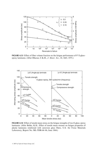
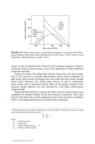
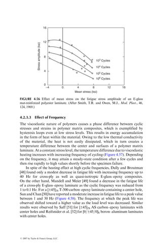
![many fatigue tests are performed until the specimen stiffness or residual
strength decreases to a predetermined level. Thus, cycles to failure may not
always represent the specimen life at complete fracture.
Many investigators have attempted to describe the S–log N plot for various
fiber-reinforced composites by a straight line:
S ¼ sU(m log N þ b), (4:23)
where
S ¼ maximum fatigue stress
N ¼ number of cycles to failure
sU ¼ average static strength
m, b ¼ constants
Values of m and b for a few epoxy matrix composites are given in Table 4.8.
A power-law representation for the S–N plot is also used:
S
sU
Nd
¼ c, (4:24)
where c and d are constants. Similar expressions can be written for «N plots
obtained in strain-controlled fatigue tests.
The number of cycles to failure, also called the fatigue life, usually exhibits a
significant degree of scatter. Following a two-parameter Weibull distribution,
the probability of fatigue life exceeding L can be written as
F(L) ¼ exp
L
L0
af
, (4:25)
TABLE 4.8
Constants in S–N Representation of Composite Laminates
Constants in Equation 4.23
Material Layup R m b References
E-glass–ductile epoxy 08 0.1 0.1573 1.3743 [26]
T-300 Carbon–ductile epoxy 08 0.1 0.0542 1.0420 [26]
E-glass–brittle epoxy 08 0.1 0.1110 1.0935 [26]
T-300 Carbon–brittle epoxy 08 0.1 0.0873 1.2103 [26]
E-glass–epoxy [0=±45=90]S 0.1 0.1201 1.1156 [27]
E-glass–epoxy [0=90]S 0.05 0.0815 0.934 [28]
Note: R represents the ratio of the minimum stress and the maximum stress in fatigue cycling.
ß 2007 by Taylor Francis Group, LLC.](https://image.slidesharecdn.com/fiberreinforcedcompositesmaterialsmanufacturinganddesignp1-220510152925-9ef3de0d/85/Fiber_Reinforced_Composites_Materials_Manufacturing_and_Design_P-1-pdf-305-320.jpg)
![where
af is the shape parameter in fatigue
L0 is the location parameter for the fatigue life distribution (cycles)
Comparing the static strength data and fatigue life data of unidirectional 08
E-glass–epoxy, Hahn and Kim [29] proposed the following correlation between
the static strength and fatigue data:
L
L0
¼
S
sU
a=af
: (4:26)
Equation 4.26 implies that the higher the static strength of a specimen, the
longer would be its fatigue life.
4.2.2 FATIGUE PERFORMANCE
4.2.2.1 Tension–Tension Fatigue
Tension–tension fatigue tests on unidirectional 08 ultrahigh-modulus carbon
fiber-reinforced thermoset polymers produce S–N curves that are almost hori-
zontal and fall within the static scatter band (Figure 4.36). The fatigue effect
is slightly greater for relatively lower modulus carbon fibers. Unidirectional 08
boron and Kevlar 49 fiber composites also exhibit exceptionally good fatigue
strength in tension–tension loading (Figure 4.37). Other laminates, such as
[0=±45=90]S carbon, [0=90]S carbon, [0=±30]S carbon, and [0=±45]S boron
Static tensile failure scatter band
High modulus carbon fibers in
a polyester matrix (vf =0.4)
(Ef =360 GPa (52.2 Msi))
R = 0
log N
Maximum
stress
(100
MPa)
0
2
4
6
8
−1 0 1 2 3 4 5 6 7
Fraction
of
tensile
strength
0
0.5
1.0
FIGURE 4.36 Tension–tension S–N diagram for a 08 ultrahigh-modulus carbon fiber–
polyester composite. (After Owen, M.J. and Morris, S., Carbon Fibres: Their Composites
and Applications, Plastics Institute, London, 1971.)
ß 2007 by Taylor Francis Group, LLC.](https://image.slidesharecdn.com/fiberreinforcedcompositesmaterialsmanufacturinganddesignp1-220510152925-9ef3de0d/85/Fiber_Reinforced_Composites_Materials_Manufacturing_and_Design_P-1-pdf-306-320.jpg)
![(Figure 4.38), show very similar S–N diagrams, although the actual fatigue
effect depends on the proportion of fibers aligned with the loading axis, stacking
sequence, and mode of cycling. The effect of cycling mode is demonstrated in
Figure 4.39, in which a tension–compression cycling (R ¼ 1.6) produces a
steeper S–N plot than the tension–tension cycling (R ¼ 0.1) and the compres-
sion–compression cycling (R ¼ 10) gives the lowest S–N plot.
The fatigue performances of both E- and S-glass fiber-reinforced compo-
sites are inferior to those of carbon, boron, and Kevlar 49 fiber-reinforced
200
0° Boron–epoxy
0° Kevlar 49–epoxy
R=0.1
Room temperature
Number of cycles to failure
Maximum
stress
(ksi)
160
120
0
103
104
105
106
107
80
40
FIGURE 4.37 Tension–tension S–N diagram for a 08 boron and Kevlar 49 fiber–epoxy
composites. (After Miner, L.H., Wolfe, R.A., and Zweben, C.H., Composite Reliability,
ASTM STP, 580, 1975.)
Number of cycles to failure
Max
stress
(ksi)
103
104
105
106
107
100
130
120
Test temperature=68⬚F
110
Frequency=32 Hz
R=0.1
+
+
+
FIGURE 4.38 Tension–tension S–N diagram for a [0=±45]S boron fiber–epoxy laminate.
(After Donat, R.C., J. Compos. Mater., 4, 124, 1970.)
ß 2007 by Taylor Francis Group, LLC.](https://image.slidesharecdn.com/fiberreinforcedcompositesmaterialsmanufacturinganddesignp1-220510152925-9ef3de0d/85/Fiber_Reinforced_Composites_Materials_Manufacturing_and_Design_P-1-pdf-307-320.jpg)
![composites. Both types of fibers produce steep S–N plots for unidirectional
08 composites (Figures 4.40 and 4.41). An improvement in their fatigue
performance can be achieved by hybridizing them with other high-modulus
fibers, such as T-300 carbon (Figure 4.42).
1000
AS carbon fiber–epoxy
Frequency = 10 Hz
[0/± 30]6S
Stress
amplitude
(MPa)
log (Cycles)
R = 0.1
R = −1.6
R = 10
0 3 4 5 6 7
800
600
400
200
0
FIGURE 4.39 S–N diagrams for [0=±30]6S AS carbon fiber–epoxy laminates at various
fatigue stress ratios (Note: R ¼ 0.1 in tension–tension cycling, R ¼ 1.6 in tension–
compression cycling, and R ¼ 10 in compression–compression cycling). (After Ramani, S.
V. and Williams, D.P., Failure Mode in Composites III, AIME, 1976.)
E-glass–epoxy R = 0.1
Maximum
stress
(10
MPa)
Cycles
107
106
105
104
103
40
80
120
18.8 Hz
34.2 Hz
FIGURE 4.40 Tension–tension S–N diagram for a 08 E-glass–epoxy laminate. (After
Hashin, Z. and Rotem, A., J. Compos. Mater., 7, 448, 1973.)
ß 2007 by Taylor Francis Group, LLC.](https://image.slidesharecdn.com/fiberreinforcedcompositesmaterialsmanufacturinganddesignp1-220510152925-9ef3de0d/85/Fiber_Reinforced_Composites_Materials_Manufacturing_and_Design_P-1-pdf-308-320.jpg)
![The tension–tension fatigue properties of SMC composites have been
reported by several investigators [30–32]. SMC materials containing E-glass
fiber-reinforced polyester or vinyl ester matrix also do not exhibit fatigue limit.
Their fatigue performance depends on the proportion of continuous and
chopped fibers in the laminate (Figure 4.43).
4.2.2.2 Flexural Fatigue
The flexural fatigue performance of fiber-reinforced composite materials is in
general less satisfactory than the tension–tension fatigue performance. This can
Frequency=25–27 Hz
R=0.5
S-glass−epoxy
103
0.1
0.3
0.5
0.7
104
Number of cycles
105 106 107
R=0.1
UTS
s
max
FIGURE 4.41 Tension–tension S–N diagram for a 08 S-glass–epoxy laminate at various
fatigue stress ratios. (After Tobler, R.L. and Read, D.L., J. Compos. Mater., 10, 32,
1976.)
160
80
0
103
104
105
106
107
Max
stress
(ksi)
R=0.1, 30 Hz
Cycles to failure
S-glass
T-300 Carbon
2:1 Hybrid
1:1 Hybrid
FIGURE 4.42 Tension–tension S–N diagram for a 08 S-glass, T-300 carbon, and
S-glass=T-300 carbon interply hybrid laminates. (After Hofer, K.E., Jr., Stander, M.,
and Bennett, L.C., Polym. Eng. Sci., 18, 120, 1978.)
ß 2007 by Taylor Francis Group, LLC.](https://image.slidesharecdn.com/fiberreinforcedcompositesmaterialsmanufacturinganddesignp1-220510152925-9ef3de0d/85/Fiber_Reinforced_Composites_Materials_Manufacturing_and_Design_P-1-pdf-309-320.jpg)
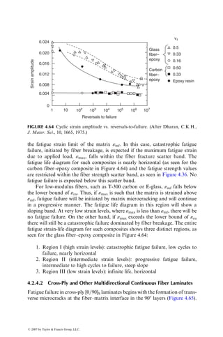
![4.2.2.3 Interlaminar Shear Fatigue
Fatigue characteristics of fiber-reinforced composite materials in the inter-
laminar shear (txz) mode have been studied by Pipes [33] and several other
investigators [34,35]. The interlaminar shear fatigue experiments were
conducted using short-beam shear specimens. For a unidirectional 08 carbon
fiber-reinforced epoxy, the interlaminar shear fatigue strength at 106
cycles was
reduced to 55% of its static ILSS even though its tension–tension fatigue
strength was nearly 80% of its static tensile strength (Figure 4.45). The inter-
laminar shear fatigue performance of a unidirectional 08 boron–epoxy system
was similar to that of unidirectional 08 carbon–epoxy system. However, a
reverse trend was observed for a unidirectional 08 S-glass-reinforced epoxy.
For this material, the interlaminar shear fatigue strength at 106
cycles was ~60%
of its static ILSS, but the tension–tension fatigue strength at 106
cycles was
40% of its static tensile strength. Unlike the static interlaminar strengths, fiber
volume fraction [34] and fiber surface treatment [35] did not exhibit any
significant influence on the high cycle interlaminar fatigue strength.
Wilson [36] has studied the interlaminar shear fatigue behavior of an SMC-
R50 laminate. His results show that the interlaminar shear fatigue strength
of this material at 106
cycles and 268C is equal to 64% of its static ILSS.
The interlaminar shear fatigue strength at 106
cycles and 908C is between 45%
and 50% of the corresponding ILSS.
HTS carbon fiber–epoxy
Glass fiber–epoxy
Fatigue
stress
Static
strength
Tension
Tension
ILS
ILS
1.0
0.8
0.6
0.4
0.2
100
101
102
103
Cycles
104
105
106
0
FIGURE 4.45 Interlaminar shear S–N diagrams for 08 carbon and glass fiber–epoxy
laminates. (After Pipes, R.B., Composite Materials: Testing and Design (Third Confe-
rence), ASTM STP, 546, 419, 1974.)
ß 2007 by Taylor Francis Group, LLC.](https://image.slidesharecdn.com/fiberreinforcedcompositesmaterialsmanufacturinganddesignp1-220510152925-9ef3de0d/85/Fiber_Reinforced_Composites_Materials_Manufacturing_and_Design_P-1-pdf-311-320.jpg)
![4.2.2.4 Torsional Fatigue
The torsional fatigue behavior of carbon fiber-reinforced epoxy thin tubes is
shown in Figure 4.46 for 08 and ±458 orientations. On a log–log scale, the S–N
plot in alternating (R ¼ 1) torsional fatigue exhibits linear behavior. The
torsional fatigue strength of ±458 specimens is ~3.7–3.8 times higher than that
of the 08 specimens at an equivalent number of cycles. The data for [0=±45]
tubes fall between the 08 and ±458 lines. The 08 specimens failed by a few
longitudinal cracks (cracks parallel to fibers), and the ±458 specimens failed
by cracking along the ±458 lines and extensive delamination. Although the 08
specimens exhibited a lower torsional fatigue strength than ±458 specimens,
they retained a much higher postfatigue static torsional strength.
Torsional fatigue data for a number of unidirectional 08 fiber-reinforced
composites are compared in Figure 4.47. The data in this figure were obtained
by shear strain cycling of solid rod specimens [37]. Fatigue testing under pure shear
conditions clearly has a severe effect on unidirectional composites, all failing at
~103
cycles at approximately half the static shear strain to failure. Short-beam
interlaminar shear fatigue experiments do not exhibit such rapid deterioration.
4.2.2.5 Compressive Fatigue
Compression–compression fatigue S–N diagram of various E-glass fiber-
reinforced polyester and epoxy composites is shown in Figure 4.48. Similar
trends are also observed for T-300 carbon fiber-reinforced epoxy systems [38].
100.0
10.0
1.0
Maximum
torsional
stress
(ksi)
0.1
103
104
105
106
Number of cycles to failure
107
108
0⬚ Unidirectional
[±45]S
FIGURE 4.46 Torsional S–N diagrams for a 08 and [±45]S high tensile strength carbon
fiber–epoxy composites. (After Fujczak, B.R., Torsional fatigue behavior of graphite–epoxy
cylinders, U.S. Army Armament Command, Report No. WVT-TR-74006, March 1974.)
ß 2007 by Taylor Francis Group, LLC.](https://image.slidesharecdn.com/fiberreinforcedcompositesmaterialsmanufacturinganddesignp1-220510152925-9ef3de0d/85/Fiber_Reinforced_Composites_Materials_Manufacturing_and_Design_P-1-pdf-312-320.jpg)
![70
60
50
40
30
20
10
0
100
101
102
Cycles to failure
G
lass−epoxy
E
p
o
x
y
r
e
s
i
n
HTS Carbon–epoxy
Kevlar 49–epoxy
High-mod. carbon–epoxy
103
104
Shear
strain
amplitude
(10
−3
)
FIGURE 4.47 Torsional shear strain-cycle diagrams for various 08 fiber-reinforced
composites. (After Phillips, D.C. and Scott, J.M., Composites, 8, 233, 1977.)
Chopped strand mat
Woven roving
[0/±45/90]S
[0/±45]S
[0/90]S
−70
−60
−50
−40
−30
−20
−10
0
0 1 2 3
log N
4 5 6
Max
compressive
stress
(ksi)
FIGURE 4.48 Compression–compression S–N diagrams for various composite lami-
nates. (After Conners, J.D., Mandell, J.F., and McGarry, F.J., Compressive fatigue in
glass and graphite reinforced composites, Proceedings 34th Annual Technical Conference,
Society of the Plastics Industry, 1979.)
ß 2007 by Taylor Francis Group, LLC.](https://image.slidesharecdn.com/fiberreinforcedcompositesmaterialsmanufacturinganddesignp1-220510152925-9ef3de0d/85/Fiber_Reinforced_Composites_Materials_Manufacturing_and_Design_P-1-pdf-313-320.jpg)
![4.2.3 VARIABLES IN FATIGUE PERFORMANCE
4.2.3.1 Effect of Material Variables
Fatigue tests on unidirectional composites containing off-axis fibers (i.e.,
u 6¼ 08) show a steady deterioration in fatigue strength with increasing
fiber orientation angle [39]. Analogous to static tests, the fatigue failure
mode in off-axis composites changes from progressive fiber failure at u 58
to matrix failure or fiber–matrix interface failure at u 58. However, a laminate
containing alternate layers of ±58 fibers has higher fatigue strength than a 08
laminate (Figure 4.49). The fatigue performance of 08 laminates is also
improved by the addition of a small percentage of 908 plies, which reduce the
tendency of splitting (cracks running parallel to fibers in the 08 laminas) due to
low transverse strengths of 08 laminas [40]. However, as the percentage of 908
plies increases, the fatigue strength is reduced.
Figure 4.50 shows the zero-tension fatigue data of two carbon fiber-
reinforced PEEK laminates, namely, [45=0=45=90]2S and [±45]4S. Higher
fatigue strength of the [45=0=45=90]2S is due to the presence of 08 fibers.
Experiments by Boller [40] and Davis et al. [41] have also shown that the
fatigue performance of laminates containing woven fabrics or randomly
oriented fibers is lower than that of unidirectional or nonwoven cross-ply lamin-
ates (Figure 4.51). Fatigue performance of laminates containing combinations
E-glass–epoxy
Zero mean stress
Frequency=15 Hz
100
80
690
552
414
276
±5⬚
±10⬚
±15⬚
0⬚
138
0
60
40
20
Alternating
stress
amplitude
(ksi)
Alternating
stress
amplitude
(MPa)
0
1 10 102
103
104
Cycles to failure
105
106
107
108
FIGURE 4.49 Effect of fiber orientation angles on the fatigue performance of E-glass–
epoxy composites. (After Boller, K.H., Mod. Plast., 41, 145, 1964.)
ß 2007 by Taylor Francis Group, LLC.](https://image.slidesharecdn.com/fiberreinforcedcompositesmaterialsmanufacturinganddesignp1-220510152925-9ef3de0d/85/Fiber_Reinforced_Composites_Materials_Manufacturing_and_Design_P-1-pdf-314-320.jpg)
![of fiber orientations, such as [0=90]S and [0=±45=90]S, are particularly sensitive
to laminate configuration, since the signs of interlaminar stresses may be
reversed by simple variations in stacking sequence (Figure 4.52).
900
600
300
0
0 2 4
log N
Maximum
stress
(MPa)
6 8
Frequency=0.5 Hz
Temperature=23⬚C
Zero–tension
Square wave
[−45/0/45/90]2S
[±45]4S
FIGURE 4.50 Zero-tension fatigue data of carbon fiber-reinforced PEEK laminates.
(After Carlile, D.R., Leach, D.C., Moore, D.R., and Zahlan, N., Advances in Thermo-
plastic Matrix Composite Materials, ASTM STP, 1044, 199, 1989.)
70
60 414
483
345
276
207
138
69
0
50
40
Alternating
stress
amplitude
(ksi)
Alternating
stress
amplitude
(MPa)
30
20
10
0
103
104
105
106
Cycles to failure
Nonwoven bias ±5⬚
Nonwoven unidirectional
Woven 181 glass fabric
Random glass fiber mat
Nonwoven cross-ply (50–50)
107
108
FIGURE 4.51 Fatigue performance of various woven fabric, nonwoven fabric, and mat-
reinforced composite laminates. (After Davis, J.W., McCarthy, J.A., and Schrub, J.N.,
Materials in Design Engineering, 1964.)
ß 2007 by Taylor Francis Group, LLC.](https://image.slidesharecdn.com/fiberreinforcedcompositesmaterialsmanufacturinganddesignp1-220510152925-9ef3de0d/85/Fiber_Reinforced_Composites_Materials_Manufacturing_and_Design_P-1-pdf-315-320.jpg)
![A systematic study of the effects of resin type and coupling agents on the
fatigue performance of fiber-reinforced polymer composites is lacking. Early
work by Boller [40] on balanced E-glass fabric-reinforced laminates has shown
the superiority of epoxies over polyesters and other thermoset resins. Mallick
[32] has shown that vinyl ester resin provides a better fatigue damage resistance
than polyester resin in an SMS-R65 laminate. However, within the same resin
category, the effects of compositional differences (e.g., low reactivity vs. high
reactivity in polyester resins or hard vs. flexible in epoxy resins) on the long-
life fatigue performance are relatively small. In zero-tension fatigue (R ¼ 0)
experiments with chopped E-glass strand mat–polyester laminates, Owen and
Rose [42] have shown that the principal effect of flexibilizing the resin is to delay
theonsetoffatiguedamage.Thelong-termfatiguelivesarenotaffectedbytheresin
flexibility.
Investigations by Tanimoto and Amijima [43] as well as Dharan [44] have
shown that, analogous to static tensile strength, the fatigue strength also
increases with increasing fiber volume fraction. An example of the effect of
fiber volume fraction is shown in Figure 4.53.
4.2.3.2 Effect of Mean Stress
The effect of tensile mean stress on the fatigue properties of fiber-
reinforced composite materials was first studied by Boller [45]. For 08 and
±158 E-glass–epoxy laminates, the stress amplitude at a constant life tends to
decrease with increasing tensile mean stress (Figure 4.54). This behavior is
70 483
414
345
276
207
138
69
0
108
107
106
105
104
103
A,B.. [±45/±15]S
C.. [±15/±45]S
20 Hz., R=0.1
b/t=8.9
2.3
A
Cycles
8.9
B
C
z
t
y
b b
Maximum
stress
(MPa)
Maximum
stress
(ksi)
60
50
40
30
20
10
0
FIGURE 4.52 Effect of laminate stacking sequence on the tension–tension fatigue
performance of carbon fiber–epoxy laminates.
ß 2007 by Taylor Francis Group, LLC.](https://image.slidesharecdn.com/fiberreinforcedcompositesmaterialsmanufacturinganddesignp1-220510152925-9ef3de0d/85/Fiber_Reinforced_Composites_Materials_Manufacturing_and_Design_P-1-pdf-316-320.jpg)
![vf
0.5
120 8
6
4
2
0
100
80
60
40
Stress
amplitude
(ksi)
Stress
amplitude
(100
MPa)
20
0
1 10 102
103
104
Reversals to failure
105
106
107
0.33
0.16
FIGURE 4.53 Effect of fiber volume fraction on the fatigue performance of 08 E-glass–
epoxy laminates. (After Dharan, C.K.H., J. Mater. Sci., 10, 1665, 1975.)
[±5⬚] Angle-ply laminate [±15⬚] Angle-ply laminate
E-glass–epoxy, 900 cycles/min (frequency)
Tensile strength
Tensile strength
103 Cycles
103
Cycles
105
Cycles
105
Cycles
10 7
Cycles
107
Cycles
Compressive
strength
Compressive strength
140
120
100
80
60
40
20
0
0 20 40 60 80 20 40 60 80 100
0
Mean tensile stress (ksi)
Alternating
stress
amplitude
(ksi)
FIGURE 4.54 Effect of tensile mean stress on the fatigue strengths of two E-glass–epoxy
laminates. (After Boller, K.H., Effect of tensile mean stresses on fatigue properties of
plastic laminates reinforced with unwoven glass fibers, U.S. Air Force Materials
Laboratory, Report No. ML-TDR-64–86, June 1964.)
ß 2007 by Taylor Francis Group, LLC.](https://image.slidesharecdn.com/fiberreinforcedcompositesmaterialsmanufacturinganddesignp1-220510152925-9ef3de0d/85/Fiber_Reinforced_Composites_Materials_Manufacturing_and_Design_P-1-pdf-317-320.jpg)
![similar to that of ductile metals. However, the Goodman equation,* which is
commonly used for ductile metals, may not be applicable for fiber-reinforced
composite materials.
Figure 4.55 shows the relationship between mean stress and stress ampli-
tude at 106
cycles for a cross-ply high-modulus carbon–epoxy composite. At
high tensile mean stresses, the fatigue curve lies within the static tensile strength
scatter band. However, low tensile mean stresses as well as compressive
mean stresses have a significant adverse effect on the fatigue strength of this
material. Similar behavior was also observed for a [0=±30]6S carbon–epoxy
composite [46].
Smith and Owen [47] have reported the effect of mean stresses on the stress
amplitude for chopped E-glass strand mat–polyester composites. Their data
(Figure 4.56) show that a small compressive mean stress may have a beneficial
effect on the fatigue performance of random fiber composites.
600
400
Stress
amplitude
(MPa)
200
Static
compressive
failure
band
Static
tensile
failure
band
0
−200 0 200
Mean stress (MPa)
400 600
FIGURE 4.55 Effect of mean stress on the fatigue strength of a cross-ply carbon fiber–
epoxy laminate. (After Owen, M.J. and Morris, S., Carbon Fibres: Their Composites and
Applications, Plastic Institute, London, 1971.)
* The Goodman equation used for taking into account the effect of tensile mean stresses for high
cycle fatigue design of metals is given by
sa
Sf
þ
sm
Sut
¼ 1,
where
sa ¼ alternating stress
sm ¼ mean stress
Sf ¼ fatigue strength with sm ¼ 0
Sut ¼ ultimate tensile strength
ß 2007 by Taylor Francis Group, LLC.](https://image.slidesharecdn.com/fiberreinforcedcompositesmaterialsmanufacturinganddesignp1-220510152925-9ef3de0d/85/Fiber_Reinforced_Composites_Materials_Manufacturing_and_Design_P-1-pdf-318-320.jpg)
![4.2.3.3 Effect of Frequency
The viscoelastic nature of polymers causes a phase difference between cyclic
stresses and strains in polymer matrix composites, which is exemplified by
hysteresis loops even at low stress levels. This results in energy accumulation
in the form of heat within the material. Owing to the low thermal conductivity
of the material, the heat is not easily dissipated, which in turn creates a
temperature difference between the center and surfaces of a polymer matrix
laminate. At a constant stress level, the temperature difference due to viscoelastic
heating increases with increasing frequency of cycling (Figure 4.57). Depending
on the frequency, it may attain a steady-state condition after a few cycles and
then rise rapidly to high values shortly before the specimen failure.
In spite of the heating effect at high cyclic frequencies, Dally and Broutman
[48] found only a modest decrease in fatigue life with increasing frequency up to
40 Hz for cross-ply as well as quasi-isotropic E-glass–epoxy composites.
On the other hand, Mandell and Meier [49] found a decrease in the fatigue life
of a cross-ply E-glass–epoxy laminate as the cyclic frequency was reduced from
1 to 0.1 Hz. For a [±45]2S T-300 carbon–epoxy laminate containing a center hole,
Sun and Chan [50] have reported a moderate increase in fatigue life to a peak value
between 1 and 30 Hz (Figure 4.58). The frequency at which the peak life was
observed shifted toward a higher value as the load level was decreased. Similar
results were observed by Saff [51] for [±45]2S AS carbon–epoxy laminates with
center holes and Reifsnider et al. [52] for [0=±45=0]S boron–aluminum laminates
with center holes.
16
12
8
4
−4 0 4 8
Mean stress (ksi)
103
Cycles
104
Cycles
105
Cycles
106
Cycles
Stress
amplitude
(ksi)
12 16
0
FIGURE 4.56 Effect of mean stress on the fatigue stress amplitude of an E-glass
mat-reinforced polyester laminate. (After Smith, T.R. and Owen, M.J., Mod. Plast., 46,
124, 1969.)
ß 2007 by Taylor Francis Group, LLC.](https://image.slidesharecdn.com/fiberreinforcedcompositesmaterialsmanufacturinganddesignp1-220510152925-9ef3de0d/85/Fiber_Reinforced_Composites_Materials_Manufacturing_and_Design_P-1-pdf-319-320.jpg)
![120
20
10
Frequency in Hz
5
1
30
40
Temperature
difference
(⬚F)
100
80
60
40
20
0
0 2,000 4,000
Time (s)
55,000
FIGURE 4.57 Difference in temperatures at the center and outside surfaces of cross-ply
E-glass–epoxy laminates during fatigue cycling. (After Dally, J.W. and Broutman, L.J.,
J. Compos. Mater., 1, 424, 1967.)
107
106
105
Load
cycles
to
failure
104
103
102
0.01 0.1 1
Load frequency (Hz)
10 100
53.3% Ultimate
57.9% Ultimate
66.6% Ultimate
FIGURE 4.58 Effect of cyclic frequency on the fatigue life of a [±45]2S carbon fiber–
epoxy laminate containing a center hole. (After Sun, C.T. and Chan, W.S., Composite
Materials, Testing and Design (Fifth Conference), ASTM STP, 674, 418, 1979.)
ß 2007 by Taylor Francis Group, LLC.](https://image.slidesharecdn.com/fiberreinforcedcompositesmaterialsmanufacturinganddesignp1-220510152925-9ef3de0d/85/Fiber_Reinforced_Composites_Materials_Manufacturing_and_Design_P-1-pdf-320-320.jpg)
![Frequency-dependent temperature rise was also detected in zero-tension
fatigue testing of carbon fiber-reinforced PEEK laminates. Temperature rise
was found to be dependent on the laminate configuration. For example, the
temperature rise in [45=0=45=90]2S laminates was only 208C above the ambi-
ent temperature, but it was up to 1508C in [±45]4S laminates, when both were
fatigue-tested at 5 Hz. Higher temperature rise in the latter was attributed to
their matrix-dominated layup. The difference in the fatigue response at 0.5 and
5 Hz for these laminate configurations is shown in Figure 4.59.
4.2.3.4 Effect of Notches
The fatigue strength of a fiber-reinforced polymer decreases with increasing notch
depth (Figure 4.60) as well as increasing notch tip sharpness (Figure 4.61). Stack-
ing sequence also plays an important role in the notch effect in fiber-reinforced
polymers. Underwood and Kendall [53] have shown that multidirectional
laminates containing 08 layers in the outer surfaces have a much longer fatigue
life than either 908 or off-axis layers in the outer surfaces.
900
600
Maximum
stress
(MPa)
300
0
0 2 4
log N
Zero-tension, square wave
6 8
, 0.5 Hz
5.0 Hz
,
[±
45]
4S
[−45/0/45/90]
2S
FIGURE 4.59 Influence of test frequency on the fatigue performance of [45=0=45=90]2S
and [±45]4S carbon fiber-reinforced PEEK laminates. (After Carlile, D.R., Leach, D.C.,
Moore, D.R., and Zahlan, N., Advances in Thermoplastic Matrix Composite Materials,
ASTM STP, 1044, 199, 1989.)
ß 2007 by Taylor Francis Group, LLC.](https://image.slidesharecdn.com/fiberreinforcedcompositesmaterialsmanufacturinganddesignp1-220510152925-9ef3de0d/85/Fiber_Reinforced_Composites_Materials_Manufacturing_and_Design_P-1-pdf-321-320.jpg)
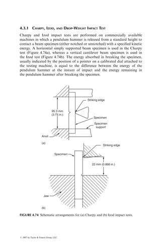
![4.2.4 FATIGUE DAMAGE MECHANISMS IN TENSION–TENSION FATIGUE TESTS
4.2.4.1 Continuous Fiber 08 Laminates
Depending on the maximum stress level, fiber type, and matrix fatigue prop-
erties, fatigue damage in continuous fiber 08 laminates is dominated either by
fiber breakage or by matrix microcracking [54–56]. At very high fatigue stress
levels, the fiber stress may exceed the lower limit of the fiber strength scatter
band. Thus, on the first application on the maximum stress, the weakest fibers
break. The locations of fiber breakage are randomly distributed in the volume
of the composite (Figure 4.62a). High stress concentration at the broken
fiber ends initiates more fiber breakage in the nearby areas. Rapidly increasing
zones of fiber failure weaken the composite severely, leading eventually to
catastrophic failure in a few hundred cycles.
At lower fatigue loads, the fiber stress may be less than the lower limit of
the fiber strength scatter band, but the matrix strain may exceed the cyclic
strain limit of the matrix. Thus failure initiation takes place by matrix
microcracking (Figure 4.62b) instead of fiber failure. High stress concentra-
tions at the ends of matrix microcracks may cause debonding at the fiber–
matrix interface and occasional fiber failure. Since the propagation of matrix
microcracks is frequently interrupted by debonding, the fatigue failure in
this region is progressive and, depending on the stress level, may span over
106
cycles.
TABLE 4.9
Comparison of Unnotched and Notched Fatigue Strengthsa
Ratio of Fatigue Strength to UTS
Unnotched Notched (Kt 5 3)b
Material
Lamination
Configuration
UTS, Mpa
(ksi)
At 104
Cycles
At 107
Cycles
At 104
Cycles
At 107
Cycles
High tensile strength
carbon fiber–epoxy
(r ¼ 1.57 g=cm3
)
08 1138 (165) 0.76 0.70 0.42 0.36
[0=90]S 759 (110) 0.71 0.59 0.57 0.55
[0=90=±45]S 400 (58) 0.83 0.78 0.55 0.52
2024-T4 aluminum
(r ¼ 2.77 g=cm3
)
— 531 (77) 0.83 0.55 0.65 0.23
Source: Adapted from Freeman, W.T. and Kuebeler, G.C., Composite Materials: Testing and
Design (Third Conference), ASTM STP, 546, 435, 1974.
a
Fatigue stress ratio R ¼ 0.1 for all experiments.
b
Kt is the theoretical stress concentration factor.
ß 2007 by Taylor Francis Group, LLC.](https://image.slidesharecdn.com/fiberreinforcedcompositesmaterialsmanufacturinganddesignp1-220510152925-9ef3de0d/85/Fiber_Reinforced_Composites_Materials_Manufacturing_and_Design_P-1-pdf-323-320.jpg)
![An important factor in determining the fatigue failure mechanism and the
nature of the fatigue life diagram in 08 laminates is the fiber stiffness [56], which
also controls the composite stiffness. For 08 composites, the composite fracture
strain «cu in the longitudinal direction is equal to the fiber fracture strain «fu.
Their scatter bands are also similar. Now, consider the tensile stress–strain
diagrams (Figure 4.63) of a high-modulus fiber composite and a low-modulus
fiber composite. For high-modulus fibers, such as GY-70 fibers, «cu is less than
(a) (b)
FIGURE 4.62 Damage development during tension–tension fatigue cycling of a 08
laminate. (a) Fiber breakage at high stress levels and (b) Matrix microcracks followed
by debonding at low stress levels.
Fiber
Fiber
efu emf
s
s
(a)
e efu
emf
(b)
e
Composite Composite
Matrix Matrix
FIGURE 4.63 Schematic longitudinal tensile stress–strain diagrams for (a) high-modulus
and (b) low-modulus 08 fiber-reinforced composite laminates. Note that «mf is the fatigue
strain limit of the matrix.
ß 2007 by Taylor Francis Group, LLC.](https://image.slidesharecdn.com/fiberreinforcedcompositesmaterialsmanufacturinganddesignp1-220510152925-9ef3de0d/85/Fiber_Reinforced_Composites_Materials_Manufacturing_and_Design_P-1-pdf-324-320.jpg)
![the fatigue strain limit of the matrix «mf. In this case, catastrophic fatigue
failure, initiated by fiber breakage, is expected if the maximum fatigue strain
due to applied load, «max, falls within the fiber fracture scatter band. The
fatigue life diagram for such composites is nearly horizontal (as seen for the
carbon fiber–epoxy composite in Figure 4.64) and the fatigue strength values
are restricted within the fiber strength scatter band, as seen in Figure 4.36. No
fatigue failure is expected below this scatter band.
For low-modulus fibers, such as T-300 carbon or E-glass, «mf falls below
the lower bound of «cu. Thus, if «max is such that the matrix is strained above
«mf, fatigue failure will be initiated by matrix microcracking and will continue
in a progressive manner. The fatigue life diagram in this region will show a
sloping band. At very low strain levels, where «max is less than «mf, there will be
no fatigue failure. On the other hand, if «max exceeds the lower bound of «cu
there will still be a catastrophic failure dominated by fiber breakage. The entire
fatigue strain-life diagram for such composites shows three distinct regions, as
seen for the glass fiber–epoxy composite in Figure 4.64:
1. Region I (high strain levels): catastrophic fatigue failure, low cycles to
failure, nearly horizontal
2. Region II (intermediate strain levels): progressive fatigue failure,
intermediate to high cycles to failure, steep slope
3. Region III (low strain levels): infinite life, horizontal
4.2.4.2 Cross-Ply and Other Multidirectional Continuous Fiber Laminates
Fatigue failure in cross-ply [0=90]S laminates begins with the formation of trans-
verse microcracks at the fiber–matrix interface in the 908 layers (Figure 4.65).
0.024
0.020
0.016
0.012
0.008
0.004
0
1 10 102
103
104
Reversals to failure
Sirain
amplitude
105
106
107
Glass
fiber–
epoxy
vf
0.5
0.33
0.16
Carbon
fiber–
epoxy
0.50
0.33
Epoxy resin
FIGURE 4.64 Cyclic strain amplitude vs. reversals-to-failure. (After Dharan, C.K.H.,
J. Mater. Sci., 10, 1665, 1975.)
ß 2007 by Taylor Francis Group, LLC.](https://image.slidesharecdn.com/fiberreinforcedcompositesmaterialsmanufacturinganddesignp1-220510152925-9ef3de0d/85/Fiber_Reinforced_Composites_Materials_Manufacturing_and_Design_P-1-pdf-325-320.jpg)
![As the cycling continues, these microcracks propagate across the 908 layers until
they reach the adjacent 08 layers. Some of the microcracks are then deflected
parallel to the 08 layers, causing delaminations between the 08 and the 908 layers.
Depending on the stress level, a number of these transverse microcracks may
appear at random locations in the first cycle; however as noted by Broutman and
Sahu [57], the transverse crack density (number of microcracks per unit area)
becomes nearly constant in a few cycles after their first appearance. It has been
found by Agarwal and Dally [28] that delaminations do not propagate for nearly
95% of the fatigue life at a given stress level. It is only during the last 5% of the
fatigue life that delaminations propagate rapidly across the 08=908 interfaces
before fiber failure in the 08 layers.
The sequence of damage development events in other multidirectional
laminates containing off-axis fibers is similar to that found in cross-ply lamin-
ates. Reifsnider et al. [58] have divided this sequence into three regions (Figure
4.66). Region I usually involves matrix microcracking through the thickness of
off-axis or 908 layers. These microcracks are parallel to fiber direction in these
layers and develop quite early in the life cycle, but they quickly stabilize to a
nearly uniform pattern with fixed spacing. The crack pattern developed in
region I is called the characteristic damage state (CDS) and is similar to that
FIGURE 4.65 Damage development during tension–tension fatigue tests of a [0=90]S
laminate.
ß 2007 by Taylor Francis Group, LLC.](https://image.slidesharecdn.com/fiberreinforcedcompositesmaterialsmanufacturinganddesignp1-220510152925-9ef3de0d/85/Fiber_Reinforced_Composites_Materials_Manufacturing_and_Design_P-1-pdf-326-320.jpg)
![observed in quasi-static loadings. The CDS is a laminate property in the sense
that it depends on the properties of individual layers, their thicknesses, and
the stacking sequence. The CDS is found to be independent of load history,
environment, residual stresses, or stresses due to moisture absorption.
Region II involves coupling and growth of matrix microcracks that ulti-
mately lead to debonding at fiber–matrix interfaces and delaminations along
layer interfaces. Both occur owing to high normal and shear stresses created at
the tips of matrix microcracks. Edge delamination may also occur in some
laminates (e.g., in [0=±45=90]S laminates) because of high interlaminar stresses
between various layers. As a result of delamination, local stresses in the 08
layers increase, since the delaminated off-axis plies cease to share the 08 load.
Additional stresses in 08 layers, in turn, cause fiber failure and accelerate the
fatigue failure process.
The principal failure mechanism in region III is the fiber fracture in 08
layers followed by debonding (longitudinal splitting) at fiber–matrix interfaces
in these layers. These fiber fractures usually develop in local areas adjacent to
the matrix microcracks in off-axis plies. It should be noted that fiber fracture
occurs in both regions II and III; however, the rate of fiber fracture is much
higher in region III, which leads quickly to laminate failure.
4.2.4.3 SMC-R Laminates
The inhomogeneous fiber distribution and random fiber orientation in SMC-R
laminates give rise to a multitude of microscopic cracking modes, such as
Residual strength
Damage development
log N
I II III
S–N
curve
1
0
S
S
ult
FIGURE 4.66 Three stages of fatigue damage development in multidirectional lami-
nates. (After Reifsnider, K., Schultz, K., and Duke, J.C., Long-Term Behavior of
Composites, ASTM STP, 813, 136, 1983.)
ß 2007 by Taylor Francis Group, LLC.](https://image.slidesharecdn.com/fiberreinforcedcompositesmaterialsmanufacturinganddesignp1-220510152925-9ef3de0d/85/Fiber_Reinforced_Composites_Materials_Manufacturing_and_Design_P-1-pdf-327-320.jpg)
![matrix cracking, fiber–matrix interfacial debonding, and fiber failure [59]. In
matrix-rich areas containing sparsely dispersed fibers, matrix cracks are formed
normal to the loading direction. Matrix cracks also develop in fiber-rich areas;
however, these cracks are shorter in length owing to close interfiber spacing.
Furthermore, if the fibers are at an angle with the loading direction, fiber–
matrix debonding is observed. Fiber fracture is rarely observed in SMC-R
laminates.
Crack density as well as average crack length in SMC-R laminates depends
strongly on the stress level. At high fatigue stress levels (60% of the ultimate
tensile strength), the crack density is high but the average crack length is small.
At lower stress levels, cracks have a lower density and longer lengths. Another
important parameter in controlling crack density and length is the resin
type [32]. This is demonstrated in Figure 4.67.
4.2.5 FATIGUE DAMAGE AND ITS CONSEQUENCES
Unlike metals, fiber-reinforced composites seldom fail along a self-similar
and well-defined crack path. Instead, fatigue damage in fiber-reinforced
composites occurs at multiple locations in the form of fiber breakage, delami-
nation, debonding, and matrix cracking or yielding. Depending on the stress
level, fiber length, fiber orientation, constituent properties, and lamination
configuration, some of these failure modes may appear either individually
or in combination quite early in the life cycle of a composite. However, they
A
B
C
Polyester
A. 2,000 Cycles, ± 15,000 psi
C. 367,000 Cycles, ± 15,000 psi
B. 40,000 Cycles, ± 15,000 psi
D. 595,000 Cycles, ± 15,000 psi
F. 375,000 Cycles, ± 20,000 psi
E. 15,000 Cycles, ± 20,000 psi
Vinyl ester
D
E
F
FIGURE 4.67 Damage development during flexural fatigue testing of SMC-R65 lami-
nates containing polyester and vinyl ester matrix. Dark lines at the center of each
specimen indicate the formation of microcracks nearly normal to the loading direction.
Note that more microcracks were formed in polyester laminates than in vinyl ester
laminates.
ß 2007 by Taylor Francis Group, LLC.](https://image.slidesharecdn.com/fiberreinforcedcompositesmaterialsmanufacturinganddesignp1-220510152925-9ef3de0d/85/Fiber_Reinforced_Composites_Materials_Manufacturing_and_Design_P-1-pdf-328-320.jpg)
![may not immediately precipitate a failure in the material. The damage grows in
size or intensity in a progressive manner until the final rupture takes place.
Figure 4.68 shows the S–N curve of a randomly oriented chopped E-glass
fiber strand mat–polyester composite in which the onset of debonding
and matrix cracking was observed two to three decades earlier than its final
rupture [60].
As the fatigue damage accumulates with cycling, the dynamic modulus of
the material is continuously decreased. This cyclic ‘‘softening’’ phenomenon
causes an increase in strain level if a stress-controlled test is used and a decrease
in stress level if a strain-controlled test is used. Because of less damage devel-
opment in a continuously reducing stress field, a strain-controlled test is
expected to produce a higher fatigue life than a stress-controlled test.
Many investigators have used the reduction in dynamic modulus as a
method of monitoring the fatigue damage development in a composite. Since
dynamic modulus can be measured frequently during fatigue cycling without
discontinuing the test or affecting the material, it is a potential nondestructive
test parameter and can be used to provide adequate warning before a structure
becomes totally ineffective [61]. Figure 4.69 shows the dynamic modulus loss of
[±45]S boron fiber–epoxy laminates in strain-controlled tension–tension fatigue
tests. Reduction in the dynamic modulus of an SMC-R in deflection-controlled
flexural fatigue tests is shown in Figure 4.70. These examples demonstrate that
the reduction in dynamic modulus depends on the stress or strain level, resin
type, and lamination configuration. Other factors that may influence the
dynamic modulus reduction are fiber type, fiber orientation angle, temperature,
Separation
Resin cracking
Debonding
Chopped strand mat E-glass−polyester
Cycles
Stress
amplitude
Tensile
strength
1.0
0.75
0.5
0.25
0
0.1 1 10 102
103
104
105
106
FIGURE 4.68 Various stages of damage growth during tension–tension fatigue cycling
of E-glass mat-reinforced polyester laminates. (After Smith, T.R. and Owen, M.J., Mod.
Plast., 46, 128, 1969.)
ß 2007 by Taylor Francis Group, LLC.](https://image.slidesharecdn.com/fiberreinforcedcompositesmaterialsmanufacturinganddesignp1-220510152925-9ef3de0d/85/Fiber_Reinforced_Composites_Materials_Manufacturing_and_Design_P-1-pdf-329-320.jpg)
![humidity, frequency, and test control mode. The significance of the fiber
orientation angle is observed in unidirectional laminates in which the dynamic
modulus reduction for u ¼ 08 orientation is considerably smaller than that for
u ¼ 908 orientation.
40
30
20
Dynamic
stiffness
loss,
percent
10
0
0 2 4 6
Cycles (105
)
emax =0.0025
emax =0.0035
emax =0.004
emax =0.005
8 10
FIGURE 4.69 Reduction in dynamic modulus during strain-controlled fatigue testing of
[±45]S boron–epoxy laminates. (After O’Brien, T.K. and Reifsnider, K.L., J. Compos.
Mater., 15, 55, 1981.)
SMC-R65 Laminates
Polyester
matrix
Vinyl ester
matrix
a. S = ± 0.56 sUF
a
1
0
20
40
102
104
Number of cycles
Reduction
in
dynamic
modulus
(percent)
106
b
c
d
e
b. S = ± 0.34 sUF
c. S = ± 0.20 sUF
d. S = ± 0.64 sUF
e. S = ± 0.38 sUF
FIGURE 4.70 Reduction in dynamic modulus during flexural fatigue cycling of SMC-
R65 laminates. (After Mallick, P.K., Polym. Compos., 2, 18, 1981.)
ß 2007 by Taylor Francis Group, LLC.](https://image.slidesharecdn.com/fiberreinforcedcompositesmaterialsmanufacturinganddesignp1-220510152925-9ef3de0d/85/Fiber_Reinforced_Composites_Materials_Manufacturing_and_Design_P-1-pdf-330-320.jpg)
![Several phenomenological models have been proposed to describe the modu-
lus reduction due to fatigue loading. One of them is due to Whitworth [62], who
suggested the following equation for calculating the residual modulus EN after N
fatigue cycles in a stress-controlled fatigue test with a maximum stress level S:
Ea
N ¼ Ea
0 H(E0 Eff)a N
Nf
, (4:27)
where
E0 ¼ initial modulus
Eff ¼ modulus at the time of fatigue failure
a, H ¼ damage parameters determined by fitting Equation 4.27 to experimen-
tal data (Figure 4.71)
Nf ¼ number of cycles to failure when the maximum stress level is S(Nf N)
If the fatigue test is conducted between fixed maximum and minimum stress
levels, then the strain level increases with fatigue cycling due to increasing
damage accumulation in the material. Assuming that the stress–strain response
of the material is linear and the fatigue failure occurs when the maximum strain
level reaches the static ultimate strain,
Eff ¼ E0
S
sU
¼ E0
S, (4:28)
where
sU ¼ ultimate static strength
S ¼ S
sU
1.0
0.9
0.8
0.7
0.6
0 0.2 0.4 0.6
Fractional life, N/Nf
Equation 4.27
[±35]2S
Modulus
reduction
ratio,
E
N
/E
0
0.8 1.0
FIGURE 4.71 Dynamic modulus reduction ratio as a function of fractional life for
[±35]2S carbon fiber–epoxy laminates (after Whitworth, H.W., ASME J. Eng. Mater.
Technol., 112, 358, 1990.)
ß 2007 by Taylor Francis Group, LLC.](https://image.slidesharecdn.com/fiberreinforcedcompositesmaterialsmanufacturinganddesignp1-220510152925-9ef3de0d/85/Fiber_Reinforced_Composites_Materials_Manufacturing_and_Design_P-1-pdf-331-320.jpg)
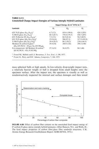
![Equation 4.32 transforms into the linear damage rule (Miner’s rule), which is
frequently used for describing damage in metals:
Miner’s rule: D ¼
X
m
i¼1
Ni
Nfi
: (4:33)
EXAMPLE 4.2
A quasi-isotropic T-300 carbon fiber–epoxy laminate is subjected to 100,000
cycles at 382 MPa after which the stress level is increased to 437 MPa. Estimate
the number of cycles the laminate will survive at the second stress level. Median
fatigue lives at 382 and 437 MPa are 252,852 and 18,922 cycles, respectively. From
the modulus vs. fatigue cycle data, the constant a and H in Equation 4.27 have
been determined as 1.47 and 1.66, respectively (see Ref. [62]). The ultimate static
strength of this material is 545 MPa.
SOLUTION
Using Equation 4.32, we can write, for failure to occur at the end of second stress
cycling,
D ¼ 1 ¼
r1
r2
N1
Nf1
þ
r2
r2
N2
Nf2
which gives,
N2 ¼ Nf2 1
r1
r2
N1
Nf1
:
In this example,
sU ¼ 545 MPa
S1 ¼ 382 MPa
Nf1 ¼ 252,852 cycles
N1 ¼ 100,000 cycles
S2 ¼ 437 MPa
Nf2 ¼ 18,922 cycles
Therefore,
r1 ¼ (1:66)
1
382
545
1:47
1
382
545
1:47
¼ 0:6917:
Similarly, r2 ¼ 0.5551
Thus,
ß 2007 by Taylor Francis Group, LLC.](https://image.slidesharecdn.com/fiberreinforcedcompositesmaterialsmanufacturinganddesignp1-220510152925-9ef3de0d/85/Fiber_Reinforced_Composites_Materials_Manufacturing_and_Design_P-1-pdf-333-320.jpg)
![N2 ¼ (18,922) 1
0:6917
0:5551
100,000
252,852
ffi 9,600 cycles:
This compares favorably with the experimental median value of 10,800 cycles [62].
4.2.6 POSTFATIGUE RESIDUAL STRENGTH
The postfatigue performance of a fiber-reinforced composite is studied by
measuring its static modulus and strength after cycling it for various fractions
of its total life. Both static modulus and strength are reduced with increasing
number of cycles. Broutman and Sahu [57] reported that much of the static
strength of a [0=90]S E-glass fiber–epoxy composite is reduced rapidly in the
first 25% of its fatigue life, which is then followed by a much slower rate of
strength reduction until the final rupture occurs (Figure 4.72). Tanimoto
and Amijima [43] also observed similar behavior for a woven E-glass cloth–
polyester laminate; however, in this case the reduction in strength takes place
only after a slight increase at 2% of the total life.
An initial increase in static strength was also observed by Reifsnider et al.
[52] for a [0=±45=0]S boron fiber–epoxy laminate containing a center hole. This
unique postfatigue behavior of a composite material was explained by means of
a wear-in and wear-out mechanism in damage development. The wear-in
process takes place in the early stages of fatigue cycling. During this process,
[0/90]S E-glass–epoxy laminates
S=0.4 sU
0
0
0.2
0.4
0.6
0.8
1.0
1 2 3 4
Number of cycles (104)
Residual
static
strength/ultimate
static
strength
5 6 7
FIGURE 4.72 Reduction in residual static strengths of [0=90]S laminates after fatigue
testing to various cycles. (After Broutman, L.J. and Sahu, S., Progressive damage of a
glass reinforced plastic during fatigue, Proceedings 20th Annual Technical Conference,
Society of the Plastics Industry, 1969.)
ß 2007 by Taylor Francis Group, LLC.](https://image.slidesharecdn.com/fiberreinforcedcompositesmaterialsmanufacturinganddesignp1-220510152925-9ef3de0d/85/Fiber_Reinforced_Composites_Materials_Manufacturing_and_Design_P-1-pdf-334-320.jpg)
![the damage developed locally around the center hole reduces the stress concen-
tration in the vicinity of the hole, thus resulting in increased strength. This
beneficial stage of fatigue cycling is followed by the wear-out process, which
comprises large-scale and widespread damage development leading to strength
reduction. Thus, the residual strength of a composite after a period of fatigue
cycling is modeled as
sresidual ¼ sU þ swear-in swear-out,
where
sU ¼ ultimate static strength
swear-in ¼ change in static strength due to wear-in
swear-out ¼ change in static strength due to wear-out
The effect of wear-in is more pronounced at high fatigue load levels. Since
fatigue life is longer at low load levels, there is a greater possibility of develop-
ing large-scale damage throughout the material. Thus, at low load levels, the
effect of wear-out is more pronounced.
A number of phenomenological equations have been proposed to predict
the residual static strength of a fatigued composite laminate [63,64]. The
simplest among them is based on the assumption of linear strength reduction
[63] and is given as
sri
¼ sUi1
(sU0
Si)
Ni
Nfi
, (4:34)
where
sri
¼ residual strength after Ni cycles at the ith stress level Si
Nfi ¼ fatigue life at Si
sU0
¼ ultimate static strength of the original laminate
sUi1
¼ ultimate static strength before being cycled at Si
In Equation 4.34, the ratio Ni=Nfi represents the fractional fatigue life
spent at Si.
Assuming a nonlinear strength degradation model, Yang [64] proposed
the following equation for the residual strength for a composite laminate
after N fatigue cycles:
sc
res ¼ sc
U sc
0KSd
N, (4:35)
where
c ¼ damage development parameter
s0 ¼ location parameter in a two-parameter Weibull function for the static
strength distribution of the laminate
S ¼ stress range in the fatigue test ¼ smaxsmin
K, d ¼ parameters used to describe the S–N diagram as KSd
Nf ¼ 1
ß 2007 by Taylor Francis Group, LLC.](https://image.slidesharecdn.com/fiberreinforcedcompositesmaterialsmanufacturinganddesignp1-220510152925-9ef3de0d/85/Fiber_Reinforced_Composites_Materials_Manufacturing_and_Design_P-1-pdf-335-320.jpg)
![Procedures for determining c, d, and K are given in Ref. [64]. It is worth
noting that, just as the static strengths, the residual strengths at the end of a
prescribed number of cycles also follow the Weibull distribution (Figure 4.73).
4.3 IMPACT PROPERTIES
The impact properties of a material represent its capacity to absorb and
dissipate energies under impact or shock loading. In practice, the impact
condition may range from the accidental dropping of hand tools to high-
speed collisions, and the response of a structure may range from localized
damage to total disintegration. If a material is strain rate sensitive, its static
mechanical properties cannot be used in designing against impact failure.
Furthermore, the fracture modes in impact conditions can be quite different
from those observed in static tests.
A variety of standard impact test methods are available for metals (ASTM
E23) and unreinforced polymers (ASTM D256). Some of these tests have also
been adopted for fiber-reinforced composite materials. However, as in the case
of metals and unreinforced polymers, the impact tests do not yield basic
material property data that can be used for design purposes. They are useful
in comparing the failure modes and energy absorption capabilities of two
different materials under identical impact conditions. They can also be used
in the areas of quality control and materials development.
Equation 4.35
Residual strength (ksi)
Distribution
function
50
0
0.2
0.4
0.6
0.8
1.0
60 70 80 90
FIGURE 4.73 Residual strength distribution in postfatigue tension tests. (After Yang,
J.N., J. Compos. Mater., 12, 19, 1978.)
ß 2007 by Taylor Francis Group, LLC.](https://image.slidesharecdn.com/fiberreinforcedcompositesmaterialsmanufacturinganddesignp1-220510152925-9ef3de0d/85/Fiber_Reinforced_Composites_Materials_Manufacturing_and_Design_P-1-pdf-336-320.jpg)
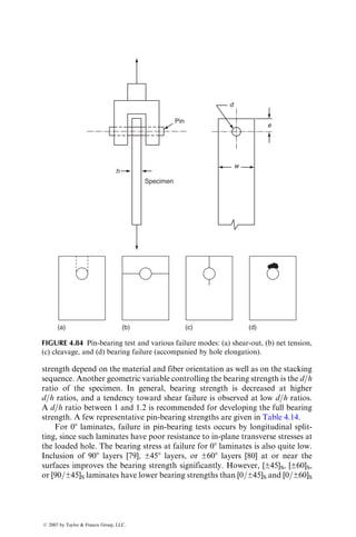
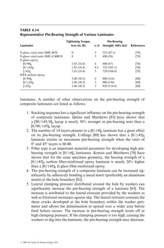
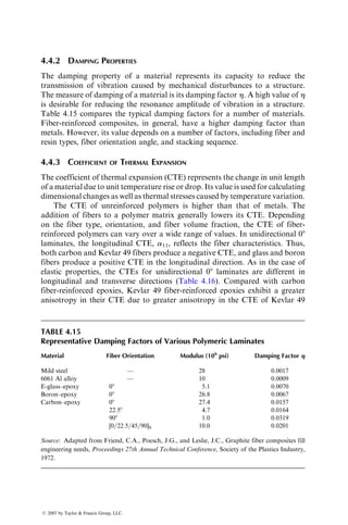
![The impact energy measured in all these tests depends on the ratio of beam
length to effective depth. Below a critical value of this ratio, there is a consider-
able increase in impact energy caused by extensive delamination [65]. The effect
of notch geometry has relatively little influence on the impact energy because
delamination at the notch root at low stresses tends to reduce its severity.
4.3.2 FRACTURE INITIATION AND PROPAGATION ENERGIES
The impact energy measured in either of the impact tests does not indicate the
fracture behavior of a material unless the relative values of fracture initiation
and propagation energies are known. Thus, for example, a high-strength brittle
material may have a high fracture initiation energy but a low fracture propa-
gation energy, and the reverse may be true for a low-strength ductile material.
Even though the sum of these two energies may be the same, their fracture
behavior is completely different. Unless the broken specimens are available for
fracture mode inspection, the toughness of a material cannot be judged by the
total impact energy alone.
Fracture initiation and propagation energies are determined from the
measurements of the dynamic load and striking head velocity during the
time of contact. Through proper instrumentation, the load and velocity signals
are integrated to produce the variation of cumulative energy as a function of
time. Both load–time and energy–time responses are recorded and are then
used for energy absorption analysis.
The load–time response during the impact test of a unidirectional composite
(Figure 4.76) can be conveniently divided into three regions [66]:
Preinitial fracture region: The preinitial fracture behavior represents
the strain energy in the beam specimen before the initial fracture occurs. In
unidirectional 08 specimens, strain energy is stored principally by the fibers.
The contribution from the matrix is negligible. The fiber strain energy Uf is
estimated as
Uf ¼
s2
f
6Ef
vf, (4:37)
where
sf ¼ longitudinal stress at the outermost fibers in the beam specimen
Ef ¼ fiber modulus
vf ¼ fiber volume fraction
This equation indicates that the energy absorption in this region can be
increased by using a low-modulus fiber and a high fiber volume fraction.
Initial fracture region: Fracture initiation at or near the peak load occurs
either by the tensile failure of the outermost fibers or by interlaminar shear
ß 2007 by Taylor Francis Group, LLC.](https://image.slidesharecdn.com/fiberreinforcedcompositesmaterialsmanufacturinganddesignp1-220510152925-9ef3de0d/85/Fiber_Reinforced_Composites_Materials_Manufacturing_and_Design_P-1-pdf-340-320.jpg)
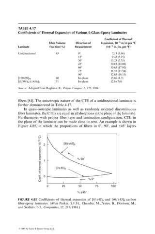
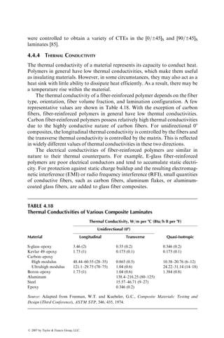
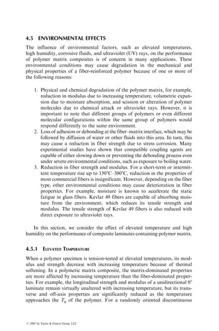
![The next important factor influencing the impact energy is the fiber–matrix
interfacial shear strength. Several investigators [69–71] have reported that
impact energy is reduced when fibers are surface-treated for improved adhesion
with the matrix. At high levels of adhesion, the failure mode is brittle and
relatively little energy is absorbed. At very low levels of adhesion, multiple
delamination may occur without significant fiber failure. Although the energy
absorption is high, failure may take place catastrophically. At intermediate
levels of adhesion, progressive delamination occurs, which in turn produces a
high impact energy absorption.
Yeung and Broutman [71] have shown that a correlation exists between the
impact energy and ILSS of a composite laminate (Figure 4.78). Different
coupling agents were used on E-glass woven fabrics to achieve various ILSSs
in short-beam shear tests. It was observed that the fracture initiation energy
increases modestly with increasing ILSS. However, the fracture propagation
energy as well as the total impact energy decrease with increasing ILSS, exhibit
a minimum, and appear to level off to intermediate values. The principal failure
mode at low ILSSs was delamination. At very high ILSSs, fiber failure was
predominant.
The strain energy contribution from the matrix in the development of
impact energy is negligible. However, the matrix can influence the impact
damage mechanism since delamination, debonding, and fiber pullout energies
depend on the fiber–matrix interfacial shear strength. Since epoxies have better
High-strength carbon fiber
in epoxy
Treated, unnotched
Untreated, unnotched
Untreated, notched Treated, notched
High-modulus carbon fiber
in epoxy
Izod
impact
energy
per
unit
width
(100
J/m)
Fiber volume fraction (%)
20
0
2
4
6
8
10
12
14
30 40 50 60 70 20 30 40 60 70
50
FIGURE 4.77 Variation of unnotched Izod impact energy with fiber volume fraction in
08 carbon–epoxy laminates. (After Hancox, N.L., Composites, 3, 41, 1971.)
ß 2007 by Taylor Francis Group, LLC.](https://image.slidesharecdn.com/fiberreinforcedcompositesmaterialsmanufacturinganddesignp1-220510152925-9ef3de0d/85/Fiber_Reinforced_Composites_Materials_Manufacturing_and_Design_P-1-pdf-344-320.jpg)
![adhesion with E-glass fibers than polyesters, E-glass–epoxy composites exhibit
higher impact energies than E-glass–polyester composites when the failure
mode is a combination of fiber failure and delamination.
In unidirectional composites, the greatest impact energy is exhibited when
the fibers are oriented in the direction of the maximum stress, that is, at 08 fiber
orientation. Any variation from this orientation reduces the load-carrying
capacity as well as the impact energy of the composite laminate. Figure 4.79
shows an example of the effect of fiber orientation on the drop-weight impact
energy of [0=90=04=0]S and [(0=90)3=0]S laminates [72]. In both cases, a min-
imum impact energy was observed at an intermediate angle between u ¼ 08 and
908. Furthermore, fracture in off-axis specimens took place principally by
interfiber cleavage parallel to the fiber direction in each layer.
The most efficient way of improving the impact energy of a low strain-
to-failure fiber composite is to hybridize it with high strain-to-failure fiber
laminas. For example, consider the GY-70 carbon fiber composite in Table
4.12 that exhibits a brittle failure mode and a low impact energy. Mallick
and Broutman [67] have shown that a hybrid sandwich composite containing
GY-70 fiber laminas in the outer skins and E-glass fiber laminas in the core has
Ut
Up
Ul
50
0
2
Interlaminar shear strength (ksi)
3 6
5 7 8
4
100
150
Unnotched
Charpy
impact
energy
(ft
lb/in.
2
)
FIGURE 4.78 Variation of unnotched Charpy impact energy with interlaminar shear
strength in E-glass fabric–polyester laminates. (After Yeung, P. and Broutman, L.J.,
Polym. Eng. Sci., 18, 62, 1978.)
ß 2007 by Taylor Francis Group, LLC.](https://image.slidesharecdn.com/fiberreinforcedcompositesmaterialsmanufacturinganddesignp1-220510152925-9ef3de0d/85/Fiber_Reinforced_Composites_Materials_Manufacturing_and_Design_P-1-pdf-345-320.jpg)
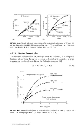
![mass spherical balls at high speeds. In low-velocity drop-weight impact tests,
a relatively heavier weight or ball is dropped from small heights onto the
specimen surface. After the impact test, the specimen is visually as well as
nondestructively inspected for internal and surface damages and then tested
TABLE 4.13
Unnotched Charpy Impact Energies of Various Interply Hybrid Laminates
Impact Energy, kJ=m2
(ft lb=in.2
)
Laminate Ui Up Ut
GY-70=E-glass: (05G=05E)S
a
6.7 (3.2) 419.6 (199.8) 426.3 (203)
T-300=E-glass: (05T=05E)S
a
60.3 (28.7) 374.4 (178.3) 434.7 (207)
GY-70=Kevlar 49: (05G=05K)S
a
7.3 (3.5) 86.9 (41.4) 94.2 (44.9)
GY-70=E-glass: [(0G=0E)5=0G]S
a
13.9 (6.6) 204 (97.2) 217.9 (103.8)
T-300=E-glass: [(0T=0E)5=0T]S
a
59.4 (28.3) 80.2 (38.2) 139.6 (66.5)
Modmor II carbon=E-glass:b
[(0E=(45=90=0=45)M)7=0E=(45=90)M]S
29.4 (14) 264.8 (126) 294.2 (140)
For comparison: All Modmor II carbon:b
[(0=45=90=0=45)7=0=45=90]S
27.3 (13) 56.8 (27) 84.1 (40)
a
From P.K. Mallick and L.J. Broutman, J. Test. Eval., 5, 190, 1977.
b
From J.L. Perry and D.F. Adams, Composites, 7, 166, 1975.
Complete break
Percentage of carbon fiber composite
Delamination and resin cracking
Unnotched
Izod
impact
energy
(J)
80
60
40
20
0
0
5
10
100
FIGURE 4.80 Effect of carbon fiber content on the unnotched Izod impact energy of
08 carbon=E-glass–epoxy interply hybrid laminates. (After Hancox, N.L. and Wells, H.,
The Izod impact properties of carbon fibre=glass fibre sandwich structures, U.K.
Atomic Energy Research Establishment Report AERE-R7016, 1972.)
ß 2007 by Taylor Francis Group, LLC.](https://image.slidesharecdn.com/fiberreinforcedcompositesmaterialsmanufacturinganddesignp1-220510152925-9ef3de0d/85/Fiber_Reinforced_Composites_Materials_Manufacturing_and_Design_P-1-pdf-347-320.jpg)
![in static tension or compression modes to determine its postimpact residual
properties.
Sidey and Bradshaw [73] performed ballistic impact experiments on
both unidirectional 08 and [(0=90)]2S carbon fiber–epoxy composites. Steel
balls, 3 mm in diameter, were impacted on 3 mm thick rectangular specimens.
The impact velocity ranged from 70 to 300 m=s. Failure mode in unidirectional
composites was longitudinal splitting (through-the-thickness cracks running
parallel to the fibers) and subsurface delamination. In cross-ply laminates, the
908 layers prevented the longitudinal cracks from running through the thickness
and restricted them to the surface layers only. Delamination was more pro-
nounced with untreated fibers.
Rhodes et al. [74] performed similar ballistic impact experiments on carbon
fiber–epoxy composites containing various arrangements of 08, 908, and ±458
laminas. Aluminum balls, 12.7 mm in diameter, were impacted on 5–8 mm
thick rectangular specimens at impact velocities ranging from 35 to 125 m=s.
Their experiments showed that, over a threshold velocity, appreciable internal
damage appeared in the impacted area even though the surfaces remained
undamaged. The principal internal damage was delamination, which was pro-
nounced at interfaces between 08 and 908 or 08 and 458 laminas. The damaged
specimens exhibited lower values of critical buckling loads and strains than the
unimpacted specimens.
Ramkumar [75] studied the effects of low-velocity drop-weight impact
tests on the static and fatigue strengths of two multidirectional AS carbon
fiber–epoxy composites. His experiments indicate that impact-induced delami-
nations, with or without visible surface damages, can severely reduce the
static compressive strengths. Static tensile strengths were affected only if dela-
minations were accompanied with surface cracks. Fatigue strengths at 106
cycles were reduced considerably more in compression–compression and
tension–compression fatigue tests than in tension–tension fatigue tests.
The growth of impact-induced delaminations toward the free edges was the
predominant failure mechanism in these fatigue tests.
Morton and Godwin [76] compared the low-velocity impact damage in
carbon fiber-reinforced [02=±45]2S and [±45=03=±45=0]S laminates containing
either a toughened epoxy or PEEK as the matrix. They observed that the
incident impact energy level to produce barely visible impact damage was
approximately equal for both toughened epoxy and PEEK composites; how-
ever, energy to produce perforation was significantly higher in PEEK compos-
ites. Nondestructive inspection of impacted laminates showed that the PEEK
laminates had less damage at or near perforation energy. Both epoxy and
PEEK laminates showed matrix cracking and ply delamination, but the latter
also exhibited local permanent deformation. Morton and Godwin [76] also
observed that the stacking sequence with 458 fibers in the outside layers pro-
vided a higher residual strength after low-energy impact than that with 08 layers
in the outside layers.
ß 2007 by Taylor Francis Group, LLC.](https://image.slidesharecdn.com/fiberreinforcedcompositesmaterialsmanufacturinganddesignp1-220510152925-9ef3de0d/85/Fiber_Reinforced_Composites_Materials_Manufacturing_and_Design_P-1-pdf-348-320.jpg)
![4.3.5 RESIDUAL STRENGTH AFTER IMPACT
If a composite laminate does not completely fail by impact loading, it may still
be able to carry loads even though it has sustained internal as well as surface
damages. The load-carrying capacity of an impact-damaged laminate is meas-
ured by testing it for residual strength in a uniaxial tension test.
The postimpact residual strength as well as the damage growth with
increasing impact velocity is shown schematically in Figure 4.81. For small
impact velocities, no strength degradation is observed (region I). As the damage
appears, the residual tensile strength is reduced with increasing impact velocity
(region II) until a minimum value is reached just before complete perforation
(region III). Higher impact velocities produce complete perforation, and the
hole diameter becomes practically independent of impact velocity (region IV).
The residual strength in this region remains constant and is equal to the
notched tensile strength of the laminate containing a hole of the same diameter
as the impacting ball. Husman et al. [77] proposed the following relationship
between the residual tensile strength in region II and the input kinetic energy:
sR ¼ sU
ffiffiffiffiffiffiffiffiffiffiffiffiffiffiffiffiffiffiffiffiffiffiffi
Us kUKE
Us
s
, (4:39)
where
sR ¼ residual tensile strength after impact
sU ¼ tensile strength of an undamaged laminate
I
II
Residual
strength
Impact velocity
III IV
Damage size
FIGURE 4.81 Schematic representation of the residual static strength in impact-
damagedlaminates.(AfterAwerbuch,J.andHahn,H.T.,J. Compos.Mater.,10,231, 1976.)
ß 2007 by Taylor Francis Group, LLC.](https://image.slidesharecdn.com/fiberreinforcedcompositesmaterialsmanufacturinganddesignp1-220510152925-9ef3de0d/85/Fiber_Reinforced_Composites_Materials_Manufacturing_and_Design_P-1-pdf-349-320.jpg)
![Us ¼ area under the stress–strain curve for an undamaged laminate
UKE ¼ input kinetic energy per unit laminate thickness
k ¼ a constant that depends on the laminate stacking sequence and
boundary conditions (e.g., one end fixed vs. both ends fixed)
Two experiments are required to determine the value of k, namely, a static
tension test on an undamaged specimen and a static tension test on an impact-
damaged specimen. Knowing the preimpact kinetic energy, the value of k can be
calculated usingEquation 4.39. Although the value of k isnot significantly affected
by the laminate thickness, it becomes independent of laminate width only for wide
specimens. Residual strength measurements on [0=90]3S laminates of various
fiber–matrix combinations have shown reasonable agreement with Equation 4.39.
4.3.6 COMPRESSION-AFTER-IMPACT TEST
The compression-after-impact test is used for assessing the nonvisible or barely
visible impact damage in composite laminates. An edge-supported quasi-
isotropic laminated plate, 153 mm 3 102 mm 3 3–5 mm thick, is impacted at
the center with an energy level of 6.7 J=mm (1500 in. lb=in.). After nondestruc-
tively examining the extent of impact damage (e.g., by ultrasonic C-scan), the
plate is compression-tested in a fixture with antibuckling guides (Figure 4.82).
The compressive strength of an impact-damaged laminate is lower than the
undamaged compressive strength. Failure modes observed in compression-
after-impact tests are shear crippling of fibers and ply delamination. In brittle
epoxy laminates, delamination is the predominant failure mode, while in
toughened epoxy matrix composites, significant shear crippling occurs before
failure by ply delamination.
Postimpact compressive strength (PICS) of a laminate can be improved by
reducing the impact-induced delamination. One way of achieving this is by
increasing the interlaminar fracture toughness of the laminate. Figure 4.83
shows that the PICS of carbon fiber-reinforced laminates increases considerably
Fixture with side
grooves to support
the composite plate
against buckling
Composite
plate with
impact
damage at
the center
Impact
damage
FIGURE 4.82 Test fixture for compression test after impact.
ß 2007 by Taylor Francis Group, LLC.](https://image.slidesharecdn.com/fiberreinforcedcompositesmaterialsmanufacturinganddesignp1-220510152925-9ef3de0d/85/Fiber_Reinforced_Composites_Materials_Manufacturing_and_Design_P-1-pdf-350-320.jpg)
![when their interlaminar fracture toughness is increased from 200 to 500 J=m2
;
however, above 1000 J=m2
, PICS is nearly independent of the interlaminar
fracture toughness. In this case, higher interlaminar fracture toughness was
obtained by increasing the fracture toughness of the matrix either by toughening
it or by changing the matrix from the standard epoxy to a thermoplastic. Other
methods of increasing the interlaminar fracture toughness and reducing ply
delamination are discussed in Section 4.7.3.
4.4 OTHER PROPERTIES
4.4.1 PIN-BEARING STRENGTH
Pin-bearing strength is an important design parameter for bolted joints and has
been studied by a number of investigators. It is obtained by tension testing a pin-
loaded hole in a flat specimen (Figure 4.84). The failure mode in pin-bearing tests
depends on a number of geometric variables [78]. Generally, at low w=d ratios,
the failure is by net tension with cracks originating at the hole boundary, and at
low e=d ratios, the failure is by shear-out. The load-carrying capacity of the
laminate is low if either of these failure modes occurs instead of bearing failure.
For bearing failure, relatively high values of w=d and e=d ratios are required.
The minimum values of w=d and e=d ratios needed to develop full bearing
400
300
200
Postimpact
compressive
strength
(MPa)
100
0
0 0.5 1.0 2.0
Interlaminar fracture toughness (kJ/m2
)
Type of carbon fiber indicated
next to each symbol
Standard epoxy
Toughened epoxy
Thermoplastic
3.0 4.0
T300
T300
T300
AS4
AS4
AS4
AS4
AS4
3K70P
AS4
AS6
IM6
IM7
FIGURE 4.83 Postimpact compressive strength of carbon fiber-reinforced laminates as a
function of their interlaminar fracture toughness (impact energy ¼ 6.7 J=mm). (Adapted
from Leach, D., Tough and damage tolerant composites, Symposium on Damage Devel-
opment and Failure Mechanisms in Composite Materials, Leuven, Belgium, 1987.)
ß 2007 by Taylor Francis Group, LLC.](https://image.slidesharecdn.com/fiberreinforcedcompositesmaterialsmanufacturinganddesignp1-220510152925-9ef3de0d/85/Fiber_Reinforced_Composites_Materials_Manufacturing_and_Design_P-1-pdf-351-320.jpg)
![strength depend on the material and fiber orientation as well as on the stacking
sequence. Another geometric variable controlling the bearing strength is the d=h
ratio of the specimen. In general, bearing strength is decreased at higher
d=h ratios, and a tendency toward shear failure is observed at low d=h ratios.
A d=h ratio between 1 and 1.2 is recommended for developing the full bearing
strength. A few representative pin-bearing strengths are given in Table 4.14.
For 08 laminates, failure in pin-bearing tests occurs by longitudinal split-
ting, since such laminates have poor resistance to in-plane transverse stresses at
the loaded hole. The bearing stress at failure for 08 laminates is also quite low.
Inclusion of 908 layers [79], ±458 layers, or ±608 layers [80] at or near the
surfaces improves the bearing strength significantly. However, [±45]S, [±60]S,
or [90=±45]S laminates have lower bearing strengths than [0=±45]S and [0=±60]S
(a) (b) (c) (d)
Pin
Specimen
h
d
e
w
FIGURE 4.84 Pin-bearing test and various failure modes: (a) shear-out, (b) net tension,
(c) cleavage, and (d) bearing failure (accompanied by hole elongation).
ß 2007 by Taylor Francis Group, LLC.](https://image.slidesharecdn.com/fiberreinforcedcompositesmaterialsmanufacturinganddesignp1-220510152925-9ef3de0d/85/Fiber_Reinforced_Composites_Materials_Manufacturing_and_Design_P-1-pdf-352-320.jpg)
![laminates. A number of other observations on the pin-bearing strength of
composite laminates are listed as follows.
1. Stacking sequence has a significant influence on the pin-bearing strength
of composite laminates. Quinn and Matthews [81] have shown that
a [90=±45=0]S layup is nearly 30% stronger in pin-bearing tests than a
[0=90=±45]S layup.
2. The number of ±u layers present in a [0=±u]S laminate has a great effect
on its pin-bearing strength. Collings [80] has shown that a [0=±45]S
laminate attains its maximum pin-bearing strength when the ratio of
08 and 458 layers is 60:40.
3. Fiber type is an important material parameter for developing high pin-
bearing strength in [0=±u]S laminates. Kretsis and Matthews [78] have
shown that for the same specimen geometry, the bearing strength of a
[0=±45]S carbon fiber-reinforced epoxy laminate is nearly 20% higher
than a [0=±45]S E-glass fiber-reinforced epoxy.
4. The pin-bearing strength of a composite laminate can be increased sig-
nificantly by adhesively bonding a metal insert (preferably an aluminum
insert) at the hole boundary [82].
5. Lateral clamping pressure distributed around the hole by washers can
significantly increase the pin-bearing strength of a laminate [83]. The
increase is attributed to the lateral restraint provided by the washers as
well as frictional resistance against slip. The lateral restraint contains the
shear cracks developed at the hole boundary within the washer peri-
meter and allows the delamination to spread over a wider area before
final failure occurs. The increase in pin-bearing strength levels off at
high clamping pressure. If the clamping pressure is too high, causing the
washers to dig into the laminate, the pin-bearing strength may decrease.
TABLE 4.14
Representative Pin-Bearing Strength of Various Laminates
Laminates
Tightening Torque,
N m (in. lb) e=d
Pin-Bearing
Strength, MPa (ksi) References
E-glass–vinyl ester SMC-R50 0 3 325 (47.1) [79]
E-glass–vinyl ester SMC-C40R30 0 3 400 (58) [79]
E-glass–epoxy
[0=90]S 1.85 (16.4) 6 600 (87) [78]
[0=±45]S 1.85 (16.4) 4.5 725 (105.1) [78]
[±45]S 1.85 (16.4) 5 720 (104.4) [78]
HTS carbon–epoxy
[0=90]S 3.40 (30.2) 6 800 (116) [80]
[0=±45]S 3.40 (30.2) 3 900 (130) [80]
[±45]S 3.40 (30.2) 5 820 (118.9) [80]
ß 2007 by Taylor Francis Group, LLC.](https://image.slidesharecdn.com/fiberreinforcedcompositesmaterialsmanufacturinganddesignp1-220510152925-9ef3de0d/85/Fiber_Reinforced_Composites_Materials_Manufacturing_and_Design_P-1-pdf-353-320.jpg)
![4.4.2 DAMPING PROPERTIES
The damping property of a material represents its capacity to reduce the
transmission of vibration caused by mechanical disturbances to a structure.
The measure of damping of a material is its damping factor h. A high value of h
is desirable for reducing the resonance amplitude of vibration in a structure.
Table 4.15 compares the typical damping factors for a number of materials.
Fiber-reinforced composites, in general, have a higher damping factor than
metals. However, its value depends on a number of factors, including fiber and
resin types, fiber orientation angle, and stacking sequence.
4.4.3 COEFFICIENT OF THERMAL EXPANSION
The coefficient of thermal expansion (CTE) represents the change in unit length
of a material due to unit temperature rise or drop. Its value is used for calculating
dimensional changes as well as thermal stresses caused by temperature variation.
The CTE of unreinforced polymers is higher than that of metals. The
addition of fibers to a polymer matrix generally lowers its CTE. Depending
on the fiber type, orientation, and fiber volume fraction, the CTE of fiber-
reinforced polymers can vary over a wide range of values. In unidirectional 08
laminates, the longitudinal CTE, a11, reflects the fiber characteristics. Thus,
both carbon and Kevlar 49 fibers produce a negative CTE, and glass and boron
fibers produce a positive CTE in the longitudinal direction. As in the case of
elastic properties, the CTEs for unidirectional 08 laminates are different in
longitudinal and transverse directions (Table 4.16). Compared with carbon
fiber-reinforced epoxies, Kevlar 49 fiber-reinforced epoxies exhibit a greater
anisotropy in their CTE due to greater anisotropy in the CTE of Kevlar 49
TABLE 4.15
Representative Damping Factors of Various Polymeric Laminates
Material Fiber Orientation Modulus (106
psi) Damping Factor h
Mild steel — 28 0.0017
6061 Al alloy — 10 0.0009
E-glass–epoxy 08 5.1 0.0070
Boron–epoxy 08 26.8 0.0067
Carbon–epoxy 08 27.4 0.0157
22.58 4.7 0.0164
908 1.0 0.0319
[0=22.5=45=90]S 10.0 0.0201
Source: Adapted from Friend, C.A., Poesch, J.G., and Leslie, J.C., Graphite fiber composites fill
engineering needs, Proceedings 27th Annual Technical Conference, Society of the Plastics Industry,
1972.
ß 2007 by Taylor Francis Group, LLC.](https://image.slidesharecdn.com/fiberreinforcedcompositesmaterialsmanufacturinganddesignp1-220510152925-9ef3de0d/85/Fiber_Reinforced_Composites_Materials_Manufacturing_and_Design_P-1-pdf-354-320.jpg)
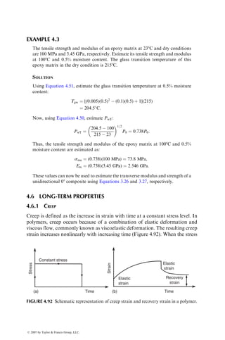
![fibers [84]. The anisotropic nature of the CTE of a unidirectional laminate is
further demonstrated in Table 4.17.
In quasi-isotropic laminates as well as randomly oriented discontinuous
fiber laminates, the CTEs are equal in all directions in the plane of the laminate.
Furthermore, with proper fiber type and lamination configuration, CTE in
the plane of the laminate can be made close to zero. An example is shown in
Figure 4.85, in which the proportions of fibers in 08, 908, and ±458 layers
TABLE 4.17
Coefficients of Thermal Expansion of Various E-Glass–Epoxy Laminates
Laminate
Fiber Volume
Fraction (%)
Direction of
Measurement
Coefficient of Thermal
Expansion, 106
m=m per 8C
(106
in.=in. per 8F)
Unidirectional 63 08 7.13 (3.96)
158 9.45 (5.25)
308 13.23 (7.35)
458 30.65 (12.08)
608 30.65 (17.03)
758 31.57 (17.54)
908 32.63 (18.13)
[±30=90]7S 60 In-plane 15.66 (8.7)
[(0=90=)9=(±45)2]S 71 In-plane 12.6 (7.0)
Source: Adapted from Raghava, R., Polym. Compos., 5, 173, 1984.
2
1
Coeff.
of
thermal
expansion
(10
−5
/°C)
0
0 25 50 75
% ±45°
[0/±45]S
[90/±45]S
% 0°
% 90⬚
100
FIGURE 4.85 Coefficients of thermal expansion of [0=±45]S and [90=±45]S carbon
fiber-epoxy laminates. (After Parker, S.F.H., Chandra, M., Yates, B., Dootson, M.,
and Walters, B.J., Composites, 12, 281, 1981.)
ß 2007 by Taylor Francis Group, LLC.](https://image.slidesharecdn.com/fiberreinforcedcompositesmaterialsmanufacturinganddesignp1-220510152925-9ef3de0d/85/Fiber_Reinforced_Composites_Materials_Manufacturing_and_Design_P-1-pdf-356-320.jpg)
![were controlled to obtain a variety of CTEs in the [0=±45]S and [90=±45]S
laminates [85].
4.4.4 THERMAL CONDUCTIVITY
The thermal conductivity of a material represents its capacity to conduct heat.
Polymers in general have low thermal conductivities, which make them useful
as insulating materials. However, in some circumstances, they may also act as a
heat sink with little ability to dissipate heat efficiently. As a result, there may be
a temperature rise within the material.
The thermal conductivity of a fiber-reinforced polymer depends on the fiber
type, orientation, fiber volume fraction, and lamination configuration. A few
representative values are shown in Table 4.18. With the exception of carbon
fibers, fiber-reinforced polymers in general have low thermal conductivities.
Carbon fiber-reinforced polymers possess relatively high thermal conductivities
due to the highly conductive nature of carbon fibers. For unidirectional 08
composites, the longitudinal thermal conductivity is controlled by the fibers and
the transverse thermal conductivity is controlled by the matrix. This is reflected
in widely different values of thermal conductivities in these two directions.
The electrical conductivities of fiber-reinforced polymers are similar in
nature to their thermal counterparts. For example, E-glass fiber-reinforced
polymers are poor electrical conductors and tend to accumulate static electri-
city. For protection against static charge buildup and the resulting electromag-
netic interference (EMI) or radio frequency interference (RFI), small quantities
of conductive fibers, such as carbon fibers, aluminum flakes, or aluminum-
coated glass fibers, are added to glass fiber composites.
TABLE 4.18
Thermal Conductivities of Various Composite Laminates
Thermal Conductivity, W=m per 8C (Btu=h ft per 8F)
Unidirectional (08)
Material Longitudinal Transverse Quasi-Isotropic
S-glass–epoxy 3.46 (2) 0.35 (0.2) 0.346 (0.2)
Kevlar 49–epoxy 1.73 (1) 0.173 (0.1) 0.173 (0.1)
Carbon–epoxy
High modulus 48.44–60.55 (28–35) 0.865 (0.5) 10.38–20.76 (6–12)
Ultrahigh modulus 121.1–29.75 (70–75) 1.04 (0.6) 24.22–31.14 (14–18)
Boron–epoxy 1.73 (1) 1.04 (0.6) 1.384 (0.8)
Aluminum 138.4–216.25 (80–125)
Steel 15.57–46.71 (9–27)
Epoxy 0.346 (0.2)
Source: Adapted from Freeman, W.T. and Kuebeler, G.C., Composite Materials: Testing and
Design (Third Conference), ASTM STP, 546, 435, 1974.
ß 2007 by Taylor Francis Group, LLC.](https://image.slidesharecdn.com/fiberreinforcedcompositesmaterialsmanufacturinganddesignp1-220510152925-9ef3de0d/85/Fiber_Reinforced_Composites_Materials_Manufacturing_and_Design_P-1-pdf-357-320.jpg)
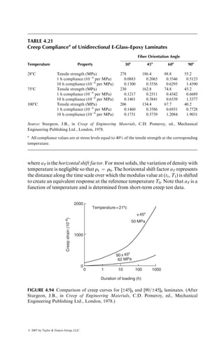
![fiber composite, strength and modulus are reduced in all directions. Reductions
in modulus as a function of increasing test temperature are shown for unidir-
ectional continuous and randomly oriented discontinuous fiber laminates in
Figures 4.86 and 4.87, respectively.
Thermal aging due to long-term exposure to elevated temperatures without
load can cause deterioration in the properties of a polymer matrix composite.
Kerr and Haskins [86] reported the effects of 100–50,000 h of thermal aging on
the tensile strength of AS carbon fiber–epoxy and HTS carbon fiber–polyimide
unidirectional and cross-ply laminates. For the AS carbon–epoxy systems,
thermal aging at 1218C produced no degradation for the first 10,000 h. Matrix
degradation began between 10,000 and 25,000 h and was severe after 50,000 h.
After 5000 h, the matrix was severely embrittled. Longitudinal tensile strength
was considerably reduced for aging times of 5000 h or longer. The HTS
carbon–polyimide systems were aged at higher temperatures but showed less
degradation than the AS carbon–epoxy systems.
Devine [87] reported the effects of thermal aging on the flexural strength
retention in SMC-R laminates containing four different thermoset polyester
resins and a vinyl ester resin. At 1308C, all SMC-R laminates retained 80%
of their respective room temperature flexural strengths even after thermal
aging for 12 months. At 1808C, all SMC-R laminates showed deterioration;
5.0
4.5
4.0
Tensile
modulus
(GPa)
1.5
1.0
0.5
0
20 40 60 80 100
Test temperature (°C)
120 140 160
0°
30°
45°
60° and 90°
Epoxy resin
FIGURE 4.86 Effect of increasing test temperature on the static tensile modulus of
unidirectional E-glass–epoxy laminates. (After Marom, G. and Broutman, L.J.,
J. Adhes., 12, 153, 1981.)
ß 2007 by Taylor Francis Group, LLC.](https://image.slidesharecdn.com/fiberreinforcedcompositesmaterialsmanufacturinganddesignp1-220510152925-9ef3de0d/85/Fiber_Reinforced_Composites_Materials_Manufacturing_and_Design_P-1-pdf-359-320.jpg)
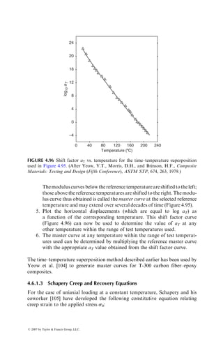
![4.5.2.1 Moisture Concentration
The moisture concentration M, averaged over the thickness, of a composite
laminate at any time during its exposure to humid environment at a given
temperature can be calculated from the following equation [88]:
M ¼ Mi þ G(Mm Mi), (4:40)
2760
0° Specimens 90° Specimens
C(23°C)
C(121°C)
T(121°C)
T(23°C)
T(121°C)
T(23°C)
C(21°C)
C(121°C)
2070
207
138
69
0
0 0.010 0.020
Strain
0.030 0.040
1380
Stress
(MPa)
Stress
(MPa)
690
0
0 0.005 0.010
Strain
(a) (b)
0.015
FIGURE 4.88 Tensile (T) and compressive (C) stress–strain diagrams of 08 and 908
carbonfiber-reinforcedPEEKlaminatesat238Cand1218C.(AfterFisher,J.M.,Palazotto,
A.N., and Sandhu, R.S., J. Compos. Technol. Res., 13, 152, 1991.)
Temperature=24°C (758F) 97% R.H.
75% R.H.
45% R.H.
T-300 carbon fiber–epoxy
4-ply laminate
10
8
6
4
Time (days)1/2
Moisture
content,
percent
weight
2
0
0
0.4
0.8
1.2
1.6
FIGURE 4.89 Moisture absorption in a carbon–epoxy laminate at 248C (758F). (After
Shen, C.H. and Springer, G.S., J. Compos. Mater., 10, 2, 1976.)
ß 2007 by Taylor Francis Group, LLC.](https://image.slidesharecdn.com/fiberreinforcedcompositesmaterialsmanufacturinganddesignp1-220510152925-9ef3de0d/85/Fiber_Reinforced_Composites_Materials_Manufacturing_and_Design_P-1-pdf-361-320.jpg)
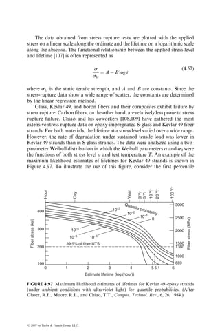
![where
Dz ¼ diffusion coefficient (mm2
=s) of the material in the direction normal to
the surface (moisture diffusion is in the thickness direction)
c ¼ laminate thickness h if both sides of the laminate are exposed to humid
environment; for exposure on one side, c ¼ 2h
t ¼ time (s)
Equation 4.42 is valid at sufficiently large values of t. For shorter times, the
average moisture concentration increases linearly with t1=2
, and the parameter
G can be approximated as
G ¼ 4
Dzt
pc2
1=2
: (4:43)
The diffusion coefficient Dz is related to the matrix diffusion coefficient Dm by
the following equation:
Dz ¼ D11 cos2
f þ D22 sin2
f, (4:44)
where
D11 ¼ Dm (1 vf)
D12 ¼ Dm 1 2
ffiffiffiffi
vf
p
q
)
Assuming fiber diffusivity (Df) matrix
diffusivity (Dm)
f ¼ fiber angle with the z direction (f ¼ 908 for fibers parallel to the
laminate surface)
vf ¼ fiber volume fraction
Equations 4.40 through 4.44 can be used to estimate the moisture concentra-
tion in a polymer matrix composite. However, the following internal and external
parameters may cause deviations from the calculated moisture concentrations.
Void content: The presence of voids has a dramatic effect on increasing the
equilibrium moisture concentration as well as the diffusion coefficient.
Fiber type: Equation 4.44 assumes that the fiber diffusivity is negligible
compared with the matrix diffusivity. This assumption is valid for glass,
carbon, and boron fibers. However, Kevlar 49 fibers are capable of absorbing
and diffusing significant amounts of moisture from the environment. As a
result, Kevlar 49 fiber-reinforced composites absorb much more moisture
than other composites.
Resin type: Moisture absorption in a resin depends on its chemical structure
and the curing agent as well as the degree of cure. Analysis of the water
absorption data of various epoxy resin compositions shows that the weight
gain due to water absorption may differ by a factor of 10 or more between
different resin chemical structures and by a factor of 3 or more for the same
resin that has different curing formulations [90]. For many resin systems,
ß 2007 by Taylor Francis Group, LLC.](https://image.slidesharecdn.com/fiberreinforcedcompositesmaterialsmanufacturinganddesignp1-220510152925-9ef3de0d/85/Fiber_Reinforced_Composites_Materials_Manufacturing_and_Design_P-1-pdf-363-320.jpg)
![the water absorption process may continue for a long time and equilibrium may
not be attained for months or even years.
Temperature: Moisture diffusion in a polymer is an energy-activated
process, and the diffusion coefficient depends strongly on the temperature
(Table 4.20). In general, the temperature dependence can be predicted from
an Arrhenius-type equation:
Dz ¼ Dz0 exp
E
RT
, (4:45)
where
E ¼ activation energy (cal=g mol)
R ¼ universal gas constant ¼ 1.987 cal=(g mol K)
T ¼ absolute temperature (K)
Dz0 ¼ a constant (mm2
=s)
Stress level: Gillat and Broutman [91] have shown that increasing the
applied stress level on a T-300 carbon–epoxy cross-ply laminate produces
higher diffusion coefficients but does not influence the equilibrium moisture
content. Similar experiments by Marom and Broutman [92] show that the
moisture absorption is a function of fiber orientation angle relative to the
loading direction. The maximum effect is observed at u ¼ 908.
Microcracks: The moisture concentration in a laminate may exceed the
equilibrium moisture concentration if microcracks develop in the material.
Moisture absorption is accelerated owing to capillary action at the microcracks
as well as exposed fiber–matrix interfaces at the laminate edges. On the other
TABLE 4.20
Diffusion Coefficients for Absorption and Desorption
in an Epoxy Resin at 100% Relative Humidity
Diffusion Coefficient (108
mm2
=s)
Temperature (8C) Absorption Desorption
0.2 3 3
25 21 17
37 41 40
50 102 88
60 179 152
70 316 282
80 411 489
90 630 661
Source: After Wright, W.W., Composites, 12, 201, 1981.
ß 2007 by Taylor Francis Group, LLC.](https://image.slidesharecdn.com/fiberreinforcedcompositesmaterialsmanufacturinganddesignp1-220510152925-9ef3de0d/85/Fiber_Reinforced_Composites_Materials_Manufacturing_and_Design_P-1-pdf-364-320.jpg)
![hand, there may be an ‘‘apparent’’ reduction in moisture concentration if there
is a loss of material from leaching or cracking.
Thermal spikes: Diffusion characteristics of composite laminates may
alter significantly if they are rapidly heated to high temperatures followed by
rapid cooling to the ambient condition, a process known as thermal spiking.
McKague et al. [93] have shown that the moisture absorption in specimens
exposed to 75% relative humidity at 248C and occasional (twice weekly) thermal
spikes (rapid heating to 1498C followed by rapid cooling to 248C) is twice that of
specimens not exposed to spikes. Additionally, thermally spiked specimens
exhibit a permanent change in their moisture absorption characteristics.
The increased diffusion rate and higher moisture absorption are attributed
to microcracks formed owing to stress gradients caused by thermal cycling and
resin swelling. The service temperature in a spike environment should be limited
to the glass transition temperature Tg of the resin, since spike temperatures
above Tg cause much higher moisture absorption than those below Tg.
Reverse thermal effect: Adamson [94] has observed that cast-epoxy resins
or epoxy-based laminates containing an equilibrium moisture concentration
exhibit a rapid rate of moisture absorption when the ambient temperature
is reduced. For example, an AS carbon fiber-reinforced epoxy laminate
attained an equilibrium moisture concentration of 2.3 wt% after 140 days of
exposure at 748C. When the exposure temperature was reduced to 258C, the
equilibrium moisture concentration increased to 2.6% within 40 days. This
inverse temperature dependence of moisture absorption is called the reverse
thermal effect.
4.5.2.2 Physical Effects of Moisture Absorption
Moisture absorption produces volumetric changes (swelling) in the resin, which
in turn cause dimensional changes in the material. Assuming that the swollen
volume of the resin is equal to the volume of absorbed water, the resulting
volume change can be computed from the following relationship:
DV(t)
V0
¼
rm
rw
M, (4:46)
where
rm ¼ matrix density
rw ¼ water density (1 kg=mm3
)
M ¼ moisture content at time t
The corresponding dilatational (volumetric) strain in the resin is
«m ¼
1
3
DV
V0
¼
1
3
rm
rw
M ¼ bmM, (4:47)
ß 2007 by Taylor Francis Group, LLC.](https://image.slidesharecdn.com/fiberreinforcedcompositesmaterialsmanufacturinganddesignp1-220510152925-9ef3de0d/85/Fiber_Reinforced_Composites_Materials_Manufacturing_and_Design_P-1-pdf-365-320.jpg)
![where
bm ¼
1
3
rm
rw
bm is called the swelling coefficient
In practice, swelling is negligible until a threshold moisture concentration
M0 is exceeded. Therefore, the dilatational strain in the resin is
«m ¼ 0 for M M0,
¼ bm(M M0) for M M0 (4:48)
The threshold moisture concentration M0 represents the amount of water
absorbed in the free volume as well as microvoids present in the resin. For a
variety of cast-epoxy resins, the measured swelling coefficient ranges from 0.26 to
0.33 and the threshold moisture concentration is in the range of 0.3%–0.7% [95].
The dilatational strain in a unidirectional 08 composite laminate due to
moisture absorption can be calculated as
Longitudinal: «mL ¼ 0, (4:49a)
Transverse: «mT ¼ bT(M Mv), (4:49b)
where
bT ¼ (1 þ nm)bm(rm=rc)
rc ¼ composite density
vm ¼ matrix Poisson’s ratio
Mv ¼ vv(rw=rc)
vv ¼ void volume fraction
Another physical effect of moisture absorption is the reduction in
glass transition temperature of the resin (Figure 4.90). Although the room-
temperature performance of a resin may not change with a reduction in Tg, its
elevated-temperature properties are severely affected. For example, the modu-
lus of an epoxy resin at 1508C decreases from 2,070 MPa (300,000 psi) to 20.7
MPa (3,000 psi) as its Tg is reduced from 2158C to 1278C. Similar effects may be
expected for the matrix-dominated properties of a polymer matrix composite.
Finally, the dilatational expansion of the matrix around the fiber reduces
the residual compressive stresses at the fiber–matrix interface caused by curing
shrinkage. As a result, the mechanical interlocking between the fiber and the
matrix may be relieved.
4.5.2.3 Changes in Performance Due to Moisture and Temperature
From the available data on the effects of temperature and moisture content on
the tensile strength and modulus of carbon and boron fiber-reinforced epoxy
laminates [96,97], the following conclusions can be made.
ß 2007 by Taylor Francis Group, LLC.](https://image.slidesharecdn.com/fiberreinforcedcompositesmaterialsmanufacturinganddesignp1-220510152925-9ef3de0d/85/Fiber_Reinforced_Composites_Materials_Manufacturing_and_Design_P-1-pdf-366-320.jpg)
![For 08 and [0=±45=90]S quasi-isotropic laminates, changes in temperature
up to 1078C (2258F) have negligible effects on tensile strength and modulus
values regardless of the moisture concentration in the material. Although the
effect on modulus is negligible up to 1778C (3508F), there may be up to a 20%
decrease in tensile strength as the temperature increases from 1078C (2258F) to
1778C (3508F).
For 08 and [0=±45=90]S laminates, the tensile strength and modulus are not
affected by moisture absorption below 1% moisture concentration. Although
the modulus is not affected by even higher moisture concentration, the tensile
strength may decrease by as much as 20% for moisture concentrations
above 1%.
For 908 laminates, increasing temperature and moisture concentration
reduce both the tensile strength and the modulus by significant amounts.
Depending on the temperature and moisture concentration, the reduction
may range as high as 60%–90% of the room temperature properties under dry
conditions.
The ILSS of composite laminates is also reduced by increasing moisture
absorption. For example, short-beam shear tests of a unidirectional carbon
fiber–epoxy show nearly a 10% reduction in ILSS at a moisture concentration
of 1.2 wt% that was attained after 33 days of exposure to humid air of 95%
relative humidity at 508C. Immersion in boiling water reduced the ILSS by 35%
500
400
300
Glass
transition
temperature
(°F)
200
100
0
2
Moisture content in epoxy (%)
4 6 8
+
+
+ +
+
+
FIGURE 4.90 Variation of glass transition temperature of various epoxy matrices
and their composites with moisture content. (After Shirrell, C.D., Halpin, J.C., and
Browning, C.E., Moisture—an assessment of its impact on the design of resin based
advanced composites, NASA Technical Report, NASA-44-TM-X-3377, April 1976.)
ß 2007 by Taylor Francis Group, LLC.](https://image.slidesharecdn.com/fiberreinforcedcompositesmaterialsmanufacturinganddesignp1-220510152925-9ef3de0d/85/Fiber_Reinforced_Composites_Materials_Manufacturing_and_Design_P-1-pdf-367-320.jpg)
![for the same exposure time [98]. Experiments by Gillat and Broutman [91] on
cross-ply carbon fiber–epoxy show nearly a 25% reduction in ILSS as the
moisture concentration increased by 1.5 wt%.
Jones et al. [99] reported the effect of moisture absorption on the tension–
tension fatigue and flexural fatigue properties of [0=90]S cross-ply epoxy matrix
composites reinforced with E-glass, HTS carbon, and Kevlar 49 fibers. Con-
ditioning treatments included exposure to humid air (65% relative humidity)
and immersion in boiling water. The fatigue resistance of carbon fiber–epoxy
was found to be unaffected by the conditioning treatment. Exposure to humid
air also did not affect the fatigue response of E-glass fiber–epoxy composites;
however, immersion in boiling water reduced the fatigue strength by significant
amounts, principally due to the damage incurred on the glass fibers by boiling
water. On the other hand, the fatigue response of Kevlar 49–epoxy composites
was improved owing to moisture absorption, although at high cycles there
appears to be a rapid deterioration as indicated by the sharp downward
curvature of the S–N curve (Figure 4.91).
Curtis and Moore [100] reported the effect of moisture absorption on the
zero tension and zero compression fatigue performance of two matrix-dominated
laminates, namely, [(90=±30)3]S and [02=452=902=þ452]S layups of carbon
fibers in an epoxy matrix. Conditioning was performed in humid air of 95%
humidity at 708C. Despite the matrix-dominated behavior of these laminates,
moisture absorption had very little effect on their fatigue lives.
Chamis et al. [101] proposed the following empirical equation for estimating
the hygrothermal effect on the matrix properties, which can subsequently be
used in modifying the matrix-dominated properties of a unidirectional lamina:
PwT
P0
¼
Tgw T
Tgd T0
1=2
, (4:50)
where
PwT ¼ matrix property at the use temperature T and moisture content M
P0 ¼ matrix property at a reference temperature T0
Tgd ¼ glass transition temperature in the dry condition
Tgw ¼ glass transition temperature in the wet condition with a moisture
content M
The glass transition temperature in the wet condition, Tgw is calculated
using the following equation:
Tgw ¼ (0:005M2
0:1M þ 1)Tgd for M 10%: (4:51)
Equations 4.50 and 4.51 have been used to estimate the hygrothermal effect on
epoxy matrix composites, but need experimental validation for other polymer
matrix systems.
ß 2007 by Taylor Francis Group, LLC.](https://image.slidesharecdn.com/fiberreinforcedcompositesmaterialsmanufacturinganddesignp1-220510152925-9ef3de0d/85/Fiber_Reinforced_Composites_Materials_Manufacturing_and_Design_P-1-pdf-368-320.jpg)
![0
0
0 2 4 6 8
2 4 6 8
0
(a)
(b)
(c)
1
0.5
0
1.0
0.5
0
0.5
1
4
2 6 8
Dry
65% RH
Boiled
Carbon–epoxy
[0/90]S
E-glass–epoxy
[0/90]S
Kevlar 49–epoxy
[0/90]S
log N
Maximum
tensile
stress
(GPa)
FIGURE 4.91 Effect of moisture absorption on the fatigue behavior of epoxy compo-
sites with (a) carbon, (b) E-glass, and (c) Kevlar 49. (After Jones, C.J., Dickson, R.F.,
Adam, T., Reiter, H., and Harris, B., Composites, 14, 288, 1983.)
ß 2007 by Taylor Francis Group, LLC.](https://image.slidesharecdn.com/fiberreinforcedcompositesmaterialsmanufacturinganddesignp1-220510152925-9ef3de0d/85/Fiber_Reinforced_Composites_Materials_Manufacturing_and_Design_P-1-pdf-369-320.jpg)

¼ 204:5
C:
Now, using Equation 4.50, estimate PwT:
PwT ¼
204:5 100
215 23
1=2
P0 ¼ 0:738P0:
Thus, the tensile strength and modulus of the epoxy matrix at 1008C and 0.5%
moisture content are estimated as:
smu ¼ (0:738)(100 MPa) ¼ 73:8 MPa,
Em ¼ (0:738)(3:45 GPa) ¼ 2:546 GPa:
These values can now be used to estimate the transverse modulus and strength of a
unidirectional 08 composite using Equations 3.26 and 3.27, respectively.
4.6 LONG-TERM PROPERTIES
4.6.1 CREEP
Creep is defined as the increase in strain with time at a constant stress level. In
polymers, creep occurs because of a combination of elastic deformation and
viscous flow, commonly known as viscoelastic deformation. The resulting creep
strain increases nonlinearly with increasing time (Figure 4.92). When the stress
(a) (b)
Strain
Stress
Constant stress
Time Time
Elastic
strain
Elastic
strain
Recovery
strain
FIGURE 4.92 Schematic representation of creep strain and recovery strain in a polymer.
ß 2007 by Taylor Francis Group, LLC.](https://image.slidesharecdn.com/fiberreinforcedcompositesmaterialsmanufacturinganddesignp1-220510152925-9ef3de0d/85/Fiber_Reinforced_Composites_Materials_Manufacturing_and_Design_P-1-pdf-370-320.jpg)
![is released after a period of time, the elastic deformation is immediately recov-
ered. The deformation caused by the viscous flow recovers slowly to an asymp-
totic value called recovery strain.
Creep strain in polymers and polymer matrix composites depends on the
stress level and temperature. Many polymers can exhibit large creep strains at
room temperature and at low stress levels. At elevated temperatures or high
stress levels, the creep phenomenon becomes even more critical. In general,
highly cross-linked thermoset polymers exhibit lower creep strains than
thermoplastic polymers. With the exception of Kevlar 49 fibers, commercial
reinforcing fibers, such as glass, carbon, and boron, do not creep [102].
4.6.1.1 Creep Data
Under uniaxial stress, the creep behavior of a polymer or a polymer matrix
composite is commonly represented by creep compliance, defined as
Creep compliance ¼ D(t) ¼
«(t)
s
, (4:52)
where
s is the constant stress level in a creep experiment
«(t) is the strain measured as a function of time
Figure 4.93 shows typical creep curves for an SMC-R25 laminate at
various stress levels. Creep compliances are determined from the slopes of
these curves. In general, creep compliance increases with time, stress level,
and temperature. For unidirectional fiber-reinforced polymers, it is also a
function of fiber orientation angle u. For u ¼ 08 creep compliance is nearly
constant, which indicates that creep in the longitudinal direction of a unidirec-
tional 08 laminate is negligible. However, at other fiber orientation angles creep
strain can be quite significant.
Fiber orientation angle also influences the temperature dependence of creep
compliance. If the fibers are in the loading direction, creep in the composite is
governed by the creep in fibers. Thus, with the exception of Kevlar 49 fibers,
little temperature dependence is expected in the fiber direction. For other fiber
orientations, creep in the matrix becomes the controlling factor. As a result,
creep compliance for off-axis laminates increases with increasing temperature
(Table 4.21). Creep in SMC-R laminates [103] containing randomly oriented
discontinuous fibers is also largely controlled by the matrix creep.
Creep in multidirectional laminates depends on the laminate construction.
For example, room temperature creep strains of [±45] and [90=±45] laminates
are nearly an order of magnitude different (Figure 4.94), even though the static
mechanical properties of these two laminates are similar. The addition of 908
layers to a ±458 construction tends to restrain the rotational tendency of ±458
fibers toward the loading direction and reduces the creep strain significantly.
ß 2007 by Taylor Francis Group, LLC.](https://image.slidesharecdn.com/fiberreinforcedcompositesmaterialsmanufacturinganddesignp1-220510152925-9ef3de0d/85/Fiber_Reinforced_Composites_Materials_Manufacturing_and_Design_P-1-pdf-371-320.jpg)
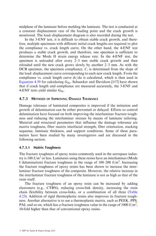
![where aT is the horizontal shift factor. For most solids, the variation of density with
temperature is negligible so that r1 ¼ r0. The horizontal shift factor aT represents
the distance along the time scale over which the modulus value at (t1, T1) is shifted
to create an equivalent response at the reference temperature T0. Note that aT is a
function of temperature and is determined from short-term creep test data.
Temperature=218c
±458
50 MPa
90±458
62 MPa
2000
1000
0
0 10 100 1000
1
Duration of loading (h)
Creep
strain
(10
−6
)
FIGURE 4.94 Comparison of creep curves for [±45]S and [90=±45]S laminates. (After
Sturgeon, J.B., in Creep of Engineering Materials, C.D. Pomeroy, ed., Mechanical
Engineering Publishing Ltd., London, 1978.)
TABLE 4.21
Creep Compliancea
of Unidirectional E-Glass–Epoxy Laminates
Fiber Orientation Angle
Temperature Property 308 458 608 908
288C Tensile strength (MPa) 278 186.4 88.8 55.2
1 h compliance (106
per MPa) 0.0883 0.2065 0.3346 0.5123
10 h compliance (106
per MPa) 0.1300 0.3356 0.6295 1.4390
758C Tensile strength (MPa) 230 162.8 74.8 43.2
1 h compliance (106
per MPa) 0.1217 0.2511 0.4342 0.6689
10 h compliance (106
per MPa) 0.1461 0.3841 0.6539 1.5377
1008C Tensile strength (MPa) 206 134.4 67.7 40.2
1 h compliance (106
per MPa) 0.1460 0.3586 0.6931 0.7728
10 h compliance (106
per MPa) 0.1751 0.5739 1.2084 1.9031
Source: Sturgeon, J.B., in Creep of Engineering Materials, C.D. Pomeroy, ed., Mechanical
Engineering Publishing Ltd., London, 1978.
a
All compliance values are at stress levels equal to 40% of the tensile strength at the corresponding
temperature.
ß 2007 by Taylor Francis Group, LLC.](https://image.slidesharecdn.com/fiberreinforcedcompositesmaterialsmanufacturinganddesignp1-220510152925-9ef3de0d/85/Fiber_Reinforced_Composites_Materials_Manufacturing_and_Design_P-1-pdf-373-320.jpg)
![The procedure for using the time–temperature superposition method is
given as follows.
1. Perform short-term (15 min–1 h) creep tests at various temperatures.
2. Plot creep modulus (or compliance) vs. log (time) for these experiments
(Figure 4.95).
3. Select a reference temperature from among the test temperatures used in
Step 1.
4. Displace the modulus curves at temperatures other than T0 horizontally
and vertically to match these curves with the modulus curve at T0.
20°C
100°C
155°C
180°C
200°C
210°C
[90]8S T-300 carbon fiber–epoxy
2.5
5.0
7.5
12.5
15.0
2.4
2.0
1.6
1.2
0.8
0.4
0
−1 2
1
10.0
Modulus
(Msi)
log Time (min)
Modulus
(GPa)
Part of
the
master
curve
FIGURE 4.95 Creep compliance curves and a portion of the master curve for a T-300
carbon–epoxy laminate. (After Yeow, Y.T., Morris, D.H., and Brinson, H.F., Compo-
site Materials: Testing and Design (Fifth Conference), ASTM STP, 674, 263, 1979.)
ß 2007 by Taylor Francis Group, LLC.](https://image.slidesharecdn.com/fiberreinforcedcompositesmaterialsmanufacturinganddesignp1-220510152925-9ef3de0d/85/Fiber_Reinforced_Composites_Materials_Manufacturing_and_Design_P-1-pdf-374-320.jpg)
![Themoduluscurvesbelow thereferencetemperatureareshiftedtothe left;
those above the reference temperatures are shifted to the right. The modu-
lus curve thus obtained is called the master curve at the selected reference
temperature and may extend over several decades of time (Figure 4.95).
5. Plot the horizontal displacements (which are equal to log aT) as
a function of the corresponding temperature. This shift factor curve
(Figure 4.96) can now be used to determine the value of aT at any
other temperature within the range of test temperatures used.
6. The master curve at any temperature within the range of test temperat-
ures used can be determined by multiplying the reference master curve
with the appropriate aT value obtained from the shift factor curve.
The time–temperature superposition method described earlier has been used by
Yeow et al. [104] to generate master curves for T-300 carbon fiber–epoxy
composites.
4.6.1.3 Schapery Creep and Recovery Equations
For the case of uniaxial loading at a constant temperature, Schapery and his
coworker [105] have developed the following constitutive equation relating
creep strain to the applied stress s0:
0
−4
0
4
8
12
16
20
24
40 80 120
Temperature (8C)
log
10
a
T
160 200 240
FIGURE 4.96 Shift factor aT vs. temperature for the time–temperature superposition
used in Figure 4.95. (After Yeow, Y.T., Morris, D.H., and Brinson, H.F., Composite
Materials: Testing and Design (Fifth Conference), ASTM STP, 674, 263, 1979.)
ß 2007 by Taylor Francis Group, LLC.](https://image.slidesharecdn.com/fiberreinforcedcompositesmaterialsmanufacturinganddesignp1-220510152925-9ef3de0d/85/Fiber_Reinforced_Composites_Materials_Manufacturing_and_Design_P-1-pdf-375-320.jpg)
![«(t) ¼ g0D(0) þ C
g1g2tn
an
s
s0, (4:55)
where
D(0) ¼ initial compliance
g0, g1, g2, as ¼ stress-dependent constants
C, n ¼ constants (independent of stress level)
During recovery after t t1, the recovery strain «r is
«r(t) ¼
D«1
g1
[(1 þ asl)n
(asl)n
], (4:56)
where
D«1 ¼
g1g2Ctn
1
an
s
s0
l ¼
t t1
t1
where t1 is the time at which the stress is released. Detailed derivations
of Equations 4.55 and 4.56 as well as the assumptions involved are given in
Ref. [105].
At low stress levels, the constants g0, g1, g2, and as are equal to unity. Creep
data obtained at low stress levels are used to determine the remaining three
constants D(0), C, and n. At high stress levels, the constants g0 6¼ g1 6¼ g2 6¼ as 6¼ 1;
however, the constants D(0), C, and n do not change.
Determination of g0, g1, g2, and as requires creep and creep recovery tests at
high stress levels. Lou and Schapery [105] have presented a graphical technique
to reduce the high-stress creep data to determine these constants. Computer-
based routines have been developed by Brinson and his coworkers and are
described in Ref. [104]. Tuttle and Brinson [106] have also presented a scheme
for predicting the long-term creep behavior of a general laminate. In this
scheme, the lamination theory (see Chapter 3) and the Schapery theory are
combined to predict the long-term creep compliance of the general laminate
from the long-term creep compliances of individual laminas.
4.6.2 STRESS RUPTURE
Stress rupture is defined as the failure of a material under sustained constant
load. It is usually performed by applying a constant tensile stress to a specimen
until it fractures completely. The time at which the fracture occurs is termed the
lifetime or stress rupture time. The objective of this test is to determine a range
of applied stresses and lifetimes within which the material can be considered
‘‘safe’’ in long-term static load applications.
ß 2007 by Taylor Francis Group, LLC.](https://image.slidesharecdn.com/fiberreinforcedcompositesmaterialsmanufacturinganddesignp1-220510152925-9ef3de0d/85/Fiber_Reinforced_Composites_Materials_Manufacturing_and_Design_P-1-pdf-376-320.jpg)
![The data obtained from stress rupture tests are plotted with the applied
stress on a linear scale along the ordinate and the lifetime on a logarithmic scale
along the abscissa. The functional relationship between the applied stress level
and lifetime [107] is often represented as
s
sU
¼ A B log t
(4:57)
where sU is the static tensile strength, and A and B are constants. Since the
stress-rupture data show a wide range of scatter, the constants are determined
by the linear regression method.
Glass, Kevlar 49, and boron fibers and their composites exhibit failure by
stress rupture. Carbon fibers, on the other hand, are relatively less prone to stress
rupture failure. Chiao and his coworkers [108,109] have gathered the most
extensive stress rupture data on epoxy-impregnated S-glass and Kevlar 49 fiber
strands. For both materials, the lifetime at a stress level varied over a wide range.
However, the rate of degradation under sustained tensile load was lower in
Kevlar 49 strands than in S-glass strands. The data were analyzed using a two-
parameter Weibull distribution in which the Weibull parameters a and s0 were
the functions of both stress level s and test temperature T. An example of the
maximum likelihood estimates of lifetimes for Kevlar 49 strands is shown in
Figure 4.97. To illustrate the use of this figure, consider the first percentile
10−3
10−4
10−5
39.5% of fiber UTS
0
100
200
300
400
Hour
Day
Year
3
Yr
5
Yr
10
Yr
20
Yr
100
Yr
3000
2500
2000
1500
1380
Fiber
stress
(MPa)
Fiber
stress
(ksi)
1000
689
1 2 3
Estimate lifetime (log (hour))
4 5 5.1 6
Quantile probability
10−6
10−2
10−1
0
FIGURE 4.97 Maximum likelihood estimates of lifetimes for Kevlar 49–epoxy strands
(under ambient conditions with ultraviolet light) for quantile probabilities. (After
Glaser, R.E., Moore, R.L., and Chiao, T.T., Compos. Technol. Rev., 6, 26, 1984.)
ß 2007 by Taylor Francis Group, LLC.](https://image.slidesharecdn.com/fiberreinforcedcompositesmaterialsmanufacturinganddesignp1-220510152925-9ef3de0d/85/Fiber_Reinforced_Composites_Materials_Manufacturing_and_Design_P-1-pdf-377-320.jpg)
![lifetime estimate of Kevlar 49 strands at 1380 MPa (200 ksi). Corresponding to
the first percentile (102
) curve, log t ffi 5.1, which gives a maximum likelihood
estimate for the lifetime as 105.1
¼ 126,000 h ¼ 14.4 years.
4.7 FRACTURE BEHAVIOR AND DAMAGE TOLERANCE
The fracture behavior of materials is concerned with the initiation and
growth of critical cracks that may cause premature failure in a structure.
In fiber-reinforced composite materials, such cracks may originate at manufac-
turing defects, such as microvoids, matrix microcracks, and ply overlaps, or at
localized damages caused by in-service loadings, such as subsurface delamina-
tions due to low-energy impacts and hole-edge delaminations due to static or
fatigue loads. The resistance to the growth of cracks that originate at the
localized damage sites is frequently referred to as the damage tolerance of
the material.
4.7.1 CRACK GROWTH RESISTANCE
Many investigators [110–112] have used the linear elastic fracture mechanics
(LEFM) approach for studying the crack growth resistance of fiber-reinforced
composite materials. The LEFM approach, originally developed for metallic
materials, is valid for crack growth with little or no plastic deformation at the
crack tip. It uses the concept of stress intensity factor KI, which is defined as
KI ¼ so
ffiffiffiffiffiffi
pa
p
Y, (4:58)
where
KI ¼ Mode I stress intensity factor (Mode I refers to the opening mode of
crack propagation due to an applied tensile stress normal to the crack
plane)
so ¼ applied stress
a ¼ crack length
Y ¼ geometric function that depends on the crack length, crack location,
and mode of loading
Equation 4.58 shows that the stress intensity factor increases with both
applied stress and crack length. An existing crack in a material may propagate
rapidly in an unstable manner (i.e., with little or no plastic deformation), when
the KI value reaches a critical level. The critical stress intensity factor, KIc, also
called the fracture toughness, indicates the resistance of the material to unstable
crack growth.
The critical stress intensity factor of metals is determined by standard test
methods, such as ASTM E399. No such standard test method is currently
available for fiber-reinforced composite materials. Most investigators have
ß 2007 by Taylor Francis Group, LLC.](https://image.slidesharecdn.com/fiberreinforcedcompositesmaterialsmanufacturinganddesignp1-220510152925-9ef3de0d/85/Fiber_Reinforced_Composites_Materials_Manufacturing_and_Design_P-1-pdf-378-320.jpg)
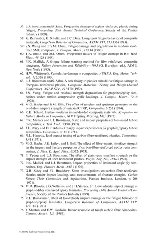
![the vicinity of the notch tip. Since the load–displacement curve deviates from
linearity, it becomes difficult to determine the load at which crack growth
begins in an unstable manner. The critical stress intensity factor calculated on
the basis of the maximum load tends to depend on the notch size, laminate
thickness, and laminate stacking sequence. Instead of using the maximum load,
Harris and Morris [110] calculated the stress intensity factor on the basis of the
load where a line drawn through the origin with 95% of the initial slope (i.e., 5%
offset from the initial slope) intercepts the load–displacement curve. Physically,
this stress intensity factor, denoted as K5, has been associated with the onset of
significant notch tip damage. Harris and Morris found the K5 value to be
relatively insensitive to the geometric variables, such as notch length, laminate
thickness, and laminate stacking sequence (Table 4.22), and called it the frac-
ture toughness of the composite material.
TABLE 4.22
Fracture Toughness of T-300 Carbon
Fiber–Epoxy Laminates
Fracture Toughness, K5 Values
Laminate Type (MPa m1=2
) (ksi in.1=2
)
[0=90=±45]S 37.0 33.7
[0=±45=90]S 33.5 30.5
[±45=0=90]S 31.4 28.6
[0=±45=90]8S 29.8 27.1
[0=±45=90]15S 29.9 27.2
[±45=0]S 32.3 29.4
[0=±45]S 32.0 29.1
[0=±45]10S 32.2 29.3
[0=±45]20S 31.6 28.8
[45=0=45]S 27.5 25.0
[0=90]S 27.8 25.3
[0=90]16S 28.7 26.1
[0=90]30S 26.6 24.2
[±30=90]S 35.7 32.5
[90=±30]S 36.4 33.1
[30=90=30]S 37.6 34.2
[90=±30]16S 28.2 25.7
[60=0=60]S 26.4 24.0
[0=±60]S 33.8 30.8
[±60=0]S 35.9 32.7
[0=±60]S 27.4 24.9
Source: Adapted from Harris, C.E. and Morris, D.H.,
J. Compos. Technol. Res., 7, 77, 1985.
ß 2007 by Taylor Francis Group, LLC.](https://image.slidesharecdn.com/fiberreinforcedcompositesmaterialsmanufacturinganddesignp1-220510152925-9ef3de0d/85/Fiber_Reinforced_Composites_Materials_Manufacturing_and_Design_P-1-pdf-380-320.jpg)
![Harris and Morris [110,113] have also observed that the fracture process in
continuous fiber laminates depends on the laminate type and laminate thickness.
For example, in thin [0=±45]nS laminates, massive delaminations at the crack tip
create uncoupling between the þ458 and 458 plies, which is followed by an
immediate failure of the laminate. The nonlinearity in the load–displacement
diagram of this laminate ensues at or near the maximum load. As the laminate
thickness increases, the thickness constraint provided by the outer layers prevents
ply delaminations at the interior layers and the notched laminate strength is
increased. In contrast, thin [0=±45=90]nS laminates develop minor delaminations
as well as matrix microcracks at the crack tip at lower than the maximum load;
however, the damage developed at the crack tip tends to relieve the stress concent-
ration in its vicinity. As a result, the load–displacement diagram for [0=±45=90]nS
laminates is more nonlinear and their notched laminate strength is also higher
than that of [0=±45]nS laminates. With increasing thickness, the size of the crack
tip damage in [0=±45=90]nS decreases and there is less stress relief in the crack tip
region, which in turn lowers the value of their notched tensile strength.
In laminates containing randomly oriented fibers, crack tip damage con-
tains matrix microcracks, fiber–matrix interfacial debonding, fiber breakage,
and so on. This damage may start accumulating at load levels as low as
50%–60% of the maximum load observed in a fracture toughness test. Thus
the load–displacement diagrams are also nonlinear for these laminates.
From the load–displacement records for various initial crack lengths, Gaggar
and Broutman [112] developed a crack growth resistance curve similar to that
given in Figure 4.100. This curve can be used to predict the stress intensity
factor at the point of unstable crack growth.
Crack growth
resistance curve
Unstable
crack growth
Crack driving
force curves
at three stress
levels
Crack length (a)
Strees
intensity
factor
(K
I
)
s3
s3 s2 s1
s2 s1
FIGURE 4.100 Crack growth resistance curve of a random fiber laminate. (After
Gaggar, S.K. and Broutman, L.J., J. Compos. Mater., 9, 216, 1975.)
ß 2007 by Taylor Francis Group, LLC.](https://image.slidesharecdn.com/fiberreinforcedcompositesmaterialsmanufacturinganddesignp1-220510152925-9ef3de0d/85/Fiber_Reinforced_Composites_Materials_Manufacturing_and_Design_P-1-pdf-381-320.jpg)
![4.7.2 DELAMINATION GROWTH RESISTANCE
Interply delamination is considered the most critical failure mode limiting the
long-term fatigue life of certain composite laminates [114]. In general, delami-
nation develops at the free edges of a laminate where adverse interlaminar
stresses may exist owing to its particular stacking sequence. Once developed,
the delaminated areas may grow steadily with increasing number of cycles,
which in turn reduces the effective modulus of the laminate. The presence of
delamination also causes a redistribution of stresses within the laminate, which
may influence the initiation of fiber breakage in the primary load-bearing plies
and reduce the fatigue life of the laminate. In recognition of this problem, a
number of test methods [115] have been developed to measure the interlaminar
fracture toughness of composite laminates.
The interlaminar fracture toughness, measured in terms of the critical strain
energy release rate, is defined as the amount of strain energy released in
propagating delamination by a unit length. This LEFM parameter is frequently
used for comparing the resistance of various resin systems against the growth of
delamination failure.
Delamination may occur in Mode I (opening mode or tensile mode of crack
propagation), Mode II (sliding mode or in-plane shear mode of crack propa-
gation), Mode III (tearing mode or antiplane shear mode of crack propaga-
tion), or a combination of these modes. The test methods used for determining
the critical strain energy release rate in Mode I and Mode II delaminations are
briefly described here. In Mode I, crack propagation occurs as the crack
surfaces pull apart due to a normal stress perpendicular to the crack plane. In
Mode II, crack propagation occurs as the crack surfaces slide over each other
due to a shear stress parallel to the crack plane. The compliance method is used
in the calculation of the strain energy release rate for each mode, which is
related to the specimen compliance by the following equation:
GI or GII ¼
P2
2w
dC
da
, (4:59)
where
P ¼ applied load
w ¼ specimen width
a ¼ crack length (measured by a traveling microscope during the test)
C ¼ specimen compliance (slope of the load–displacement curve for each
crack length) (see Figure 4.102)
dC
da ¼ slope of the compliance vs. crack length curve
The interlaminar fracture toughness, GIc in Mode I and GIIc in Mode II, are
calculated using the critical load Pc and dC
da corresponding to the crack length at
the onset of delamination propagation.
ß 2007 by Taylor Francis Group, LLC.](https://image.slidesharecdn.com/fiberreinforcedcompositesmaterialsmanufacturinganddesignp1-220510152925-9ef3de0d/85/Fiber_Reinforced_Composites_Materials_Manufacturing_and_Design_P-1-pdf-382-320.jpg)
![4.7.2.1 Mode I Delamination
Two commonly used Mode I interlaminar fracture energy tests are the double-
cantilever beam (DCB) test and the edge delamination tension (EDT) test.
DCB test: The DCB test is used for determining the strain energy release
rate GI for delamination growth under Mode I loading. It commonly uses a
straight-sided 08 unidirectional specimen (Figure 4.101) in which an initial
crack (delamination) is created by inserting a thin Teflon film (typically 0.013
mm thick) at the midplane before molding the laminate. Hinged metal tabs are
bonded at the delaminated end of the specimen. Load is applied through the
metal tabs until the initial crack grows slowly by a predetermined length. The
specimen is unloaded and then reloaded until the new crack in the specimen
grows slowly by another predetermined length. This process is repeated several
times with the same specimen to obtain a series of load–displacement records,
as shown in Figure 4.102. For each crack length, a specimen compliance value
is calculated using the slope of the loading portion of the corresponding load–
displacement record. A typical compliance vs. crack length curve is shown in
Figure 4.103.
EDT test: The EDT test uses a straight-sided 11-ply [(30)2=90=90]S
laminate that exhibits free-edge delaminations at both 308=908 interfaces
under a tensile load. It involves determining the laminate stiffness ELAM and
Initial crack Laminate
Hinged end tab
P
P
FIGURE 4.101 A double-cantilever beam (DCB) specimen.
ß 2007 by Taylor Francis Group, LLC.](https://image.slidesharecdn.com/fiberreinforcedcompositesmaterialsmanufacturinganddesignp1-220510152925-9ef3de0d/85/Fiber_Reinforced_Composites_Materials_Manufacturing_and_Design_P-1-pdf-383-320.jpg)
![the normal strain «c at the onset of delamination from the stress–strain diagram
(Figure 4.104) obtained in a static tension test of the [(30)2=90=90]S laminate.
The critical strain energy release rate at the onset of delamination is then
calculated using the following equation [116]:
Δd
Δd
d
d
ΔP
ΔP Compliance (C) =
a1
a0
a0
a1
a2
a2
P
P
P
FIGURE 4.102 Typical load–displacement records obtained in a DCB test.
dC
da
at crack
length ai
ai
Crack length (mm or in.)
Compliance,
C
(m/N
or
in./lb)
FIGURE 4.103 Schematic representation of compliance vs. crack length in a DCB test.
ß 2007 by Taylor Francis Group, LLC.](https://image.slidesharecdn.com/fiberreinforcedcompositesmaterialsmanufacturinganddesignp1-220510152925-9ef3de0d/85/Fiber_Reinforced_Composites_Materials_Manufacturing_and_Design_P-1-pdf-384-320.jpg)
![GIc ¼
«2
ct
2
(ELAM E*), (4:60)
where
h ¼ specimen thickness
«c ¼ strain at the onset of delamination
ELAM ¼ initial laminate stiffness
E* ¼ [8E(30)þ þ 3E(90)]=11
The E* term in Equation 4.60 represents a simple rule of mixture calcula-
tion for the laminate stiffness after complete delamination has taken place at
both 308=908 interfaces.
Both DCB and EDT tests are useful in qualitatively ranking various matrix
materials for their role in delamination growth resistance of a laminate. Both
tests produce comparable results (Figure 4.105). In general, the delamination
growth resistance increases with increasing fracture toughness of the matrix;
however, improving the fracture toughness of a matrix may not translate into
an equivalent increase in the delamination growth of a laminate.
4.7.2.2 Mode II Delamination
End notched flexure tests are used to determine the interlaminar fracture
toughness in Mode II delamination of [0] unidirectional laminates. There are
two types of end notched flexure tests: (a) 3-point or 3-ENF test and (b) 4-point
or 4-ENF test. The specimen and loading configurations for these two tests are
shown in Figure 4.106. In both specimens, a starter crack is created at one end
of the specimen by placing a thin Teflon film (typically 0.013 mm thick) at the
Extensometer
100 mm (4 in.)
254 mm
(10 in.)
178 mm
(7 in.)
s
s
s
38 mm (1.5 in.)
ec e
ELAM
FIGURE 4.104 An edge delamination tension (EDT) test.
ß 2007 by Taylor Francis Group, LLC.](https://image.slidesharecdn.com/fiberreinforcedcompositesmaterialsmanufacturinganddesignp1-220510152925-9ef3de0d/85/Fiber_Reinforced_Composites_Materials_Manufacturing_and_Design_P-1-pdf-385-320.jpg)
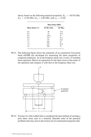
![midplane of the laminate before molding the laminate. The test is conducted at
a constant displacement rate of the loading point and the crack growth is
monitored. The load–displacement diagram is also recorded during the test.
In the 3-ENF test, it is difficult to obtain stable crack growth, and there-
fore, multiple specimens with different initial crack lengths are required to plot
the compliance vs. crack length curve. On the other hand, the 4-ENF test
produces a stable crack growth, and therefore, one specimen is sufficient to
determine the Mode II strain energy release rate. In the 4-ENF test, the
specimen is unloaded after every 2–3 mm stable crack growth and then
reloaded until the new crack grows slowly by another 2–3 mm. As with the
DCB specimen, the specimen compliance, C, is determined from the slope of
the load–displacement curve corresponding to each new crack length. From the
compliance vs. crack length curve dc=da is calculated, which is then used in
Equation 4.59 for calculating GIIc. Schuecker and Davidson [117] have shown
that if crack length and compliance are measured accurately, the 3-ENF and
4-ENF tests yield similar GIIc.
4.7.3 METHODS OF IMPROVING DAMAGE TOLERANCE
Damage tolerance of laminated composites is improved if the initiation and
growth of delamination can be either prevented or delayed. Efforts to control
delamination have focused on both improving the interlaminar fracture tough-
ness and reducing the interlaminar stresses by means of laminate tailoring.
Material and structural parameters that influence the damage tolerance are
matrix toughness, fiber–matrix interfacial strength, fiber orientation, stacking
sequence, laminate thickness, and support conditions. Some of these para-
meters have been studied by many investigators and are discussed in the
following section.
4.7.3.1 Matrix Toughness
The fracture toughness of epoxy resins commonly used in the aerospace indus-
try is 100 J=m2
or less. Laminates using these resins have an interlaminar (Mode
I delamination) fracture toughness in the range of 100–200 J=m2
. Increasing
the fracture toughness of epoxy resins has been shown to increase the inter-
laminar fracture toughness of the composite. However, the relative increase in
the interlaminar fracture toughness of the laminate is not as high as that of the
resin itself.
The fracture toughness of an epoxy resin can be increased by adding
elastomers (e.g., CTBN), reducing cross-link density, increasing the resin
chain flexibility between cross-links, or a combination of all three (Table
4.23). Addition of rigid thermoplastic resins also improves its fracture tough-
ness. Another alternative is to use a thermoplastic matrix, such as PEEK, PPS,
PAI, and so on, which has a fracture toughness value in the range of 1000 J=m2
,
10-fold higher than that of conventional epoxy resins.
ß 2007 by Taylor Francis Group, LLC.](https://image.slidesharecdn.com/fiberreinforcedcompositesmaterialsmanufacturinganddesignp1-220510152925-9ef3de0d/85/Fiber_Reinforced_Composites_Materials_Manufacturing_and_Design_P-1-pdf-387-320.jpg)
![4.7.3.2 Interleaving
A second approach of enhancing the interlaminar fracture toughness is to add a
thin layer of tough, ductile polymer or adhesive between each consecutive plies
in the laminate [118] (Figure 4.107). Although the resin-rich interleaves increase
the interlaminar fracture toughness, fiber-dominated properties, such as tensile
TABLE 4.23
Mode I Interlaminar Fracture Toughness as Influenced by the Matrix
Composition
Matrix Properties Composite Propertiesa
General Feature
of the Base Resin
Tensile
Strain-to-
Failure (%) GIc (J=m2
) vf (%)
Transverse
Tensile Strain-
to-Failure (%) GIc (J=m2
)
Rigid TGMDA=DDS epoxy 1.34 70 76 0.632 190
Moderately cross-linked with
rigid backbone between
cross-links
1.96 167 54 0.699 335
Same as above plus CTBN
rubber particles
3.10 730 60 0.580 1015
69 520
71 615
Epoxy with low cross-link
density and soft backbone
between cross-links
3.24 460 58 0.538 455
Same as above plus CTBN
rubber particles
18.00 5000 57 0.538 1730
Source: Adapted from Jordan, W.M., Bradley, W.L., and Moulton, R.J., J. Compos. Mater., 23,
923, 1989.
a
08 Unidirectional carbon fiber-reinforced epoxy composites.
Adhesive
layers
(a) (b)
FIGURE 4.107 Interleaving with adhesive layers (a) along the whole laminate width and
(b) along the free edges only.
ß 2007 by Taylor Francis Group, LLC.](https://image.slidesharecdn.com/fiberreinforcedcompositesmaterialsmanufacturinganddesignp1-220510152925-9ef3de0d/85/Fiber_Reinforced_Composites_Materials_Manufacturing_and_Design_P-1-pdf-388-320.jpg)
![strength and modulus, may decrease due to a reduction in overall fiber volume
fraction.
4.7.3.3 Stacking Sequence
High interlaminar normal and shear stresses at the free edges of a laminate are
created due to mismatch of Poisson’s ratios and coefficients of mutual influence
between adjacent layers. Changing the ply stacking sequence may change
the interlaminar normal stress from tensile to compressive so that opening
mode delamination can be suppressed. However, the growth of delamination
may require the presence of an interrupted load path. For example, Lee and
Chan [119] used discrete 908 plies at the midplanes of [30=302=30]S
and [±35=0]S laminates to reduce delamination in these laminates. Delamina-
tion was arrested at the boundaries of these discrete plies.
4.7.3.4 Interply Hybridization
This can also be used to reduce the mismatch of Poisson’s ratios and coeffi-
cients of mutual influence between consecutive layers, and thus reduce the
possibility of interply edge delamination. For example, replacing the 908 carbon
fiber–epoxy plies in [±45=02=902]S AS-4 carbon fiber–epoxy laminates with 908
E-glass fiber–epoxy plies increases the stress level for the onset of edge delami-
nation (due to interlaminar normal stress, szz) from 324 to 655 MPa.
The ultimate tensile strength is not affected, since it is controlled mainly by
the 08 plies, which are carbon fiber–epoxy for both laminates [120].
4.7.3.5 Through-the-Thickness Reinforcement
Resistance to interlaminar delamination can be improved by means of through-
the-thickness reinforcement that can be in the form of stitches, metallic wires
and pins, or three-dimensional fabric structures.
Mignery et al. [121] used fine Kevlar thread to stitch the layers in [±30=0]S,
[±30=90]S, and [±45=02=90]S AS-4 carbon fiber–epoxy laminates. Stitches par-
allel to the 08 direction were added after layup with an industrial sewing
machine at a distance of 1.3–2.5 mm from the free edges in 32 mm wide test
specimens. Although stitching did not prevent the occurrence of free-edge
delamination in uniaxial tensile tests, it substantially reduced the rate of
delamination growth into the interior of the latter two laminates. No visible
edge delamination occurred in either unstitched or stitched [±30=0]S laminates
before complete fracture.
Figure 4.108 shows the construction of a three-dimensional composite
containing alternate 0=90 layers in the laminate plane (xy plane) and vertical
through-the-thickness fibers interlocked with the in-plane layers. Gillespie and
his coworkers [122] reported a 10-fold increase in the Mode I interlaminar
ß 2007 by Taylor Francis Group, LLC.](https://image.slidesharecdn.com/fiberreinforcedcompositesmaterialsmanufacturinganddesignp1-220510152925-9ef3de0d/85/Fiber_Reinforced_Composites_Materials_Manufacturing_and_Design_P-1-pdf-389-320.jpg)
![fracture toughness of such three-dimensional composites over the two-dimen-
sional 0=90 laminates; however, the in-plane stiffness properties are decreased.
4.7.3.6 Ply Termination
High interlaminar stresses created by mismatching plies in a narrow region near
the free edge are reduced if they are terminated away from the free edge. Chan
and Ochoa [123] tension tested [±35=0=09]S laminates in which the 908 layers
were terminated at ~3.2 mm away from the free edges of the tension specimen
and found no edge delamination up to the point of laminate failure. The
ultimate tensile strength of the laminate with 908 ply terminations was 36%
higher than the baseline laminate without ply termination. In the baseline
laminate, free-edge delamination between the central 908 layers was observed
at 49% of the ultimate load.
4.7.3.7 Edge Modification
Sun and Chu [124] introduced a series of narrow and shallow (1.6–3.2 mm deep)
notches (Figure 4.109) along the laminate edges and observed a significant
z
908 0⬚
FIGURE 4.108 Construction of a three-dimensional laminate.
Machined notches along
the free edges of a laminate
FIGURE 4.109 Edge notched laminate.
ß 2007 by Taylor Francis Group, LLC.](https://image.slidesharecdn.com/fiberreinforcedcompositesmaterialsmanufacturinganddesignp1-220510152925-9ef3de0d/85/Fiber_Reinforced_Composites_Materials_Manufacturing_and_Design_P-1-pdf-390-320.jpg)
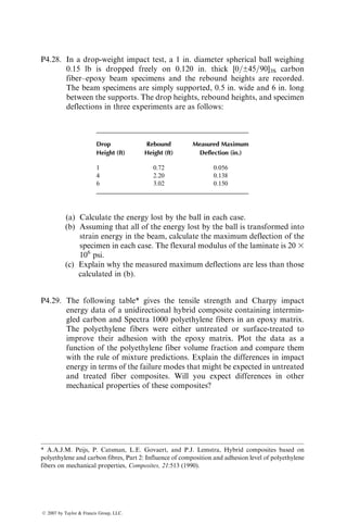
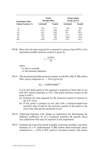
![36. D.W. Wilson, Characterization of the interlaminar shear fatigue properties of
SMC-R50, Technical Report No. 80–05, Center for Composite Materials, Univer-
sity of Delaware, Newark, DE (1980).
37. D.C. Phillips and J.M. Scott, The shear fatigue of unidirectional fibre composites,
Composites, 8:233 (1977).
38. J.D. Conners, J.F. Mandell, and F.J. McGarry, Compressive fatigue in glass and
graphite reinforced composites, Proceedings 34th Annual Technical Conference,
Society of the Plastics Industry (1979).
39. Z. Hashin and A. Rotem, A fatigue failure criterion for fiber reinforced materials,
J. Compos. Mater., 7:448 (1973).
40. K.H. Boller, Fatigue characteristics of RP laminates subjected to axial loading,
Mod. Plast., 41:145 (1964).
41. J.W. Davis, J.A. McCarthy, and J.N. Schrub, The fatigue resistance of reinforced
plastics, Materials in Design Engineering, p. 87 (1964).
42. M.J. Owen and R.G. Rose, Polyester flexibility versus fatigue behavior of RP,
Mod. Plast., 47:130 (1970).
43. T. Tanimoto and S. Amijima, Progressive nature of fatigue damage of glass fiber
reinforced plastics, J. Compos. Mater., 9 (1975).
44. C.K.H. Dharan, Fatigue failure in graphite fibre and glass fibre-polymer compos-
ites, J. Mater. Sci., 10:1665 (1975).
45. K.H. Boller, Effect of tensile mean stresses on fatigue properties of plastic lamin-
ates reinforced with unwoven glass fibers, U.S. Air Force Materials Laboratory,
Report No. ML-TDR-64–86, June (1964).
46. S.V. Ramani and D.P. Williams, Axial fatigue of [0=±30]6S graphite=epoxy, Failure
Mode in Composites III, AIME, p. 115 (1976).
47. T.R. Smith and M.J. Owen, Fatigue properties of RP, Mod. Plast., 46:124
(1969).
48. J.W. Dally and L.J. Broutman, Frequency effects on the fatigue of glass reinforced
plastics, J. Compos. Mater., 1:424 (1967).
49. J.F. Mandell and U. Meier, Effects of stress ratio, frequency, and loading time on
the tensile fatigue of glass-reinforced epoxy, Long-Term Behavior of Composites,
ASTM STP, 813:55 (1983).
50. C.T. Sun and W.S. Chan, Frequency effect on the fatigue life of a laminated
composite, Composite Materials, Testing and Design (Fifth Conference), ASTM
STP, 674:418 (1979).
51. C.R. Saff, Effect of load frequency and lay-up on fatigue life of composites, Long-
Term Behavior of Composites, ASTM STP, 813:78 (1983).
52. K.L. Reifsnider, W.W. Stinchcomb, and T.K. O’Brien, Frequency effects on a
stiffness-based fatigue failure criterion in flawed composite specimens, Fatigue of
Filamentary Composite Materials, ASTM STP, 636: 171 (1977).
53. J.H. Underwood and D.P. Kendall, Fatigue damage in notched glass–epoxy sheet,
Proceedings International Conference on Composite Materials, Vol. 2, AIME,
p. 1122 (1975).
54. C.K.H. Dharan, Fatigue failure mechanisms in a unidirectionally reinforced com-
posite material, Fatigue of Composite Materials, ASTM STP, 569:171 (1975).
55. H.C. Kim and L.J. Ebert, Axial fatigue failure sequence and mechanisms in
unidirectional fiberglass composites, J. Compos. Mater., 12:139 (1978).
56. R. Talreja, Fatigue of composite materials: damage mechanisms and fatigue-life
diagrams, Proc. R. Soc. Lond., A, 378:461 (1981).
ß 2007 by Taylor Francis Group, LLC.](https://image.slidesharecdn.com/fiberreinforcedcompositesmaterialsmanufacturinganddesignp1-220510152925-9ef3de0d/85/Fiber_Reinforced_Composites_Materials_Manufacturing_and_Design_P-1-pdf-393-320.jpg)
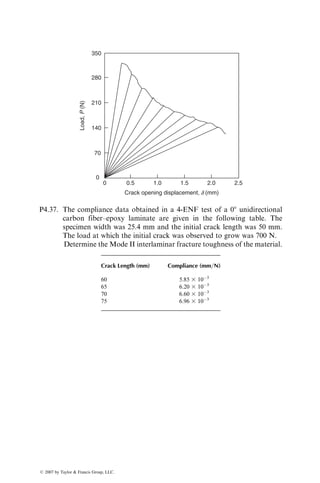
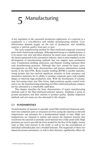
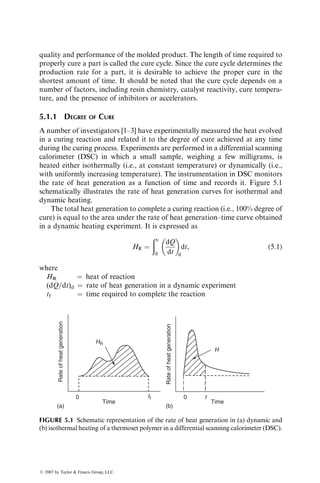
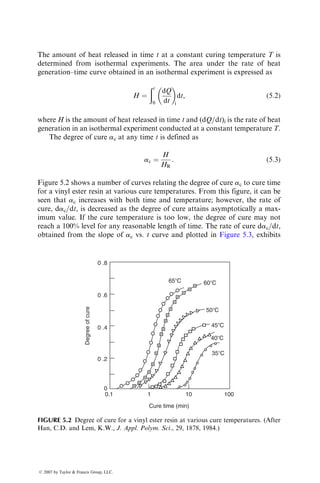
![Using the following material properties, calculate the corrected tensile
modulus values at each L=w and compare them with the theoretical
modulus: E11 ¼ 20 3 106
psi, E22 ¼ 1 3 106
psi, n12 ¼ 0.25, and G12 ¼
0.6 3 106
psi.
P4.3. The following longitudinal tensile strength data (in MPa) were obtained
for a [0=±45=90]S E-glass fiber–epoxy laminate: 520.25, 470.27, 457.60,
541.18, 566.35, 489.82, 524.55, 557.87, 490.00, 498.99, 496.95, 510.84,
and 558.76.
(a) Determine the average tensile strength, the standard deviation, and
coefficient of variation
(b) Determine the Weibull parameters for the given strength distribu-
tion
(c) Using the Weibull parameters in (b), determine the mean strength
for the material
P4.4. The tensile stress–strain diagram for a [(0=90)2=0=90]S E-glass fiber–
epoxy laminate is shown in the figure. Determine the initial modulus,
the stress at the knee point, the secondary modulus, and the failure
strength for the laminate. Compare these experimental values with the
theoretical estimates.
C
B
A
A: 0⬚
C: 90⬚
B: [(0/90)2/0/90]S
Strain
Stress
10
ksi
0.01 in./in.
ß 2007 by Taylor Francis Group, LLC.](https://image.slidesharecdn.com/fiberreinforcedcompositesmaterialsmanufacturinganddesignp1-220510152925-9ef3de0d/85/Fiber_Reinforced_Composites_Materials_Manufacturing_and_Design_P-1-pdf-398-320.jpg)
![P4.5. Tensile stress–strain diagram of a [0=904]S AS-4 carbon fiber–epoxy
laminate is shown in the figure. The longitudinal modulus and trans-
verse modulus of a 08 unidirectional laminate of the same material are
142 and 10.3 GPa, respectively.
1. Determine the initial axial modulus of the [0=904]S laminate and
compare it with the theoretical value. How would this value change
if the 908 layers are at the outside or the laminate construction is
changed to [02=903]S?
2. The knee in the stress–strain diagram is at a strain of 0.005 mm=mm.
However, the ultimate longitudinal and transverse strains of the 08
unidirectional laminate are at 0.0146 and 0.006 mm=mm, respect-
ively. Explain what might have caused a lower strain at the knee
3. Describe the reason for the nonlinear portion of the stress–strain
diagram
0
0
100
200
300
400
500
0.3 0.6 0.9 1.2
Strain (percent)
Stress
(MPa)
1.5 1.8
P4.6. The longitudinal compressive strength of a unidirectional 08 carbon
fiber–epoxy laminate is estimated as 190 ksi. Using the Euler buckling
formula for homogeneous materials, design the minimum thickness of a
Celanese compression specimen that will be required to avoid lateral
buckling.
P4.7. The following compressive strength data were obtained for a 08 uni-
directional surface-treated high-strength carbon fiber–epoxy composite
tested in the longitudinal (fiber) direction.* The composite specimens
failed by shear cracks at 458 to the axis of loading.
* N.L. Hancox, The compression strength of unidirectional carbon fibre reinforced plastic,
J. Mater. Sci., 10:234 (1975).
ß 2007 by Taylor Francis Group, LLC.](https://image.slidesharecdn.com/fiberreinforcedcompositesmaterialsmanufacturinganddesignp1-220510152925-9ef3de0d/85/Fiber_Reinforced_Composites_Materials_Manufacturing_and_Design_P-1-pdf-399-320.jpg)
![vf (%) sLCU (MPa)
10 325
20 525
30 712
40 915
50 1100
60 1250
70 1750
Plot the data and verify that the compressive strength is linear with vf.
Assuming that the rule of mixture applies, determine the longitudinal
compressive strength of the carbon fiber. How may the compressive
strength and failure mode of the composite be affected by matrix
strength and fiber surface treatment?
P4.8. The following tensile stress–strain values were obtained in uniaxial
tensile testing of a [±45]S laminate:
sxx (MPa) «xx (mm=mm) «yy (mm=mm)
27.5 0.001 0.00083
54.4 0.002 0.00170
82.7 0.003 0.00250
96.5 0.004 0.00340
115.7 0.005 0.00700
132.5 0.006 0.00811
161.0 0.007 0.00905
214.0 0.014 0.01242
Plot the data and determine the Exx and nxy of the laminate. In
addition, reduce the data to plot t12 vs. g12 for the material and
determine G12.
P4.9. Using the stress and strain transformation Equations 3.30 and 3.31, verify
Equations 4.16 and 4.17 for the 108 off-axis test shown in Figure 4.28.
P4.10. The following table* gives the stress–strain data for [0=90=±45]S and
[0=90]2S AS-4 carbon fiber–epoxy laminates obtained in a three-rail
shear test. Plot the data and determine the shear modulus for each
laminate. Compare these values with those predicted by the lamination
* S. Tan and R. Kim, Fracture of composite laminates containing cracks due to shear loading, Exp.
Mech., 28:364 (1988).
ß 2007 by Taylor Francis Group, LLC.](https://image.slidesharecdn.com/fiberreinforcedcompositesmaterialsmanufacturinganddesignp1-220510152925-9ef3de0d/85/Fiber_Reinforced_Composites_Materials_Manufacturing_and_Design_P-1-pdf-400-320.jpg)
![theory based on the following material properties: E11 ¼ 143.92 GPa,
E22 ¼ 11.86 GPa, G12 ¼ 6.68 GPa, and n12 ¼ 0.326.
Shear Stress (MPa)
Shear Strain (%) [0=90=±45]S [0=90]2S
0.2 40 13.6
0.4 91 24.5
0.6 128.6 37
0.8 155 47.3
1.0 178 54.5
1.2 208 62
1.4 232 65.4
1.6 260 70
P4.11. The following figure shows the schematic of an asymmetric four-point
bend (AFPB) test developed for measuring the shear properties of
composite laminates. As in the Iosipescu shear test, it uses a V-notched
beam specimen. Derive an expression for the shear stress at the center of
the specimen and compare it with that in the Iosipescu shear test.
V-notched
specimen
w
P
L
a
P4.12. Torsion of a thin-walled tube is considered the best method of creating a
pure shear stress state in a material. Describe some of the practical
problems that may arise in the torsion test of a laminated composite tube.
ß 2007 by Taylor Francis Group, LLC.](https://image.slidesharecdn.com/fiberreinforcedcompositesmaterialsmanufacturinganddesignp1-220510152925-9ef3de0d/85/Fiber_Reinforced_Composites_Materials_Manufacturing_and_Design_P-1-pdf-401-320.jpg)
![P4.18. Some investigators have proposed using a four-point flexure test for
ILSS measurements. Using the homogeneous beam theory, develop
equations for ILSS in a four-point flexure test and discuss the merits
of such a test over a three-point short-beam shear test.
P4.19. Using Table 4.8, compare the fatigue strengths of T-300 carbon–epoxy
and E-glass–epoxy composites at 104
and 107
cycles.
P4.20. The Weibull parameters for the tension–tension fatigue life distribution
of a [0=90=±45]S T-300 carbon fiber–epoxy composite are as follows: at
smax ¼ 340 MPa, L0 ¼ 1,000,000, and af ¼ 1.6. At smax ¼ 410 MPa,
L0 ¼ 40,000, and af ¼ 1.7.
1. Determine the mean fatigue lives at 340 and 410 MPa
2. What is the expected probability of surviving 50,000 cycles at 410 MPa?
P4.21. Fatigue lives (numbers of cycles to failure) of twelve 08 Kevlar 49 fiber-
reinforced composite specimens in tension–tension cycling at 90% UTS,
R ¼ 0.1, 0.5 Hz frequency, and 238C are reported as 1,585; 25; 44,160;
28,240; 74,140; 47; 339,689; 50,807; 320,415; 865; 5,805; and 4,930. Plot
the Weibull distribution curve for these fatigue lives and determine the
Weibull parameters for this distribution.
P4.22. For the major portion of the fatigue life of a composite laminate, the
instantaneous modulus can be modeled as
E ¼ E0(1 c log N)
where
E0 ¼ initial modulus at N ¼ 1
N ¼ number of fatigue cycles
c ¼ an experimentally determined damage-controlling factor
Using this model, determine the number of cycles that a simply sup-
ported centrally loaded beam can endure before its deflection becomes
50% higher than its initial value.
P4.23. For the quasi-isotropic laminate described in Example 4.2, suppose
the loading sequence is 10,000 cycles at 437 MPa followed by cycling
to failure at 382 MPa. Estimate the total life expected in this high–
low stress sequence using (a) the Whitworth model and (b) the
Miner’s rule.
P4.24. The mean fatigue lives of [0=90]S E-glass fiber–epoxy laminates at
maximum stress levels of 56,000 and 35,000 psi are 1,500 and 172,000,
respectively. The static tensile strength of this material is 65,000 psi.
ß 2007 by Taylor Francis Group, LLC.](https://image.slidesharecdn.com/fiberreinforcedcompositesmaterialsmanufacturinganddesignp1-220510152925-9ef3de0d/85/Fiber_Reinforced_Composites_Materials_Manufacturing_and_Design_P-1-pdf-403-320.jpg)
![1. Determine the residual static strength of this material after 50% of
the fatigue life at each stress level
2. After cycling for 50% of the fatigue life at 35,000 psi, the maximum
stress level in a fatigue specimen is increased to 56,000 psi. Estimate
the number of cycles the specimen would survive at 56,000 psi
3. If the first stress level is 56,000 psi, which is then followed by 35,000
psi, estimate the number of cycles at the second stress level
P4.25. Adam et al.* have found that, depending on the fiber type, the post-
fatigue residual strength of [0=90] cross-plied composites may show
either a gradual decrease with increasing number of cycles (usually
after a rapid reduction in the first few cycles) or virtually no change
until they fail catastrophically (sudden death). They proposed the
following empirical equation to predict the residual strength:
sres ¼ smax(sU smax)(1 rx
)1=y
,
where
r ¼
log N log 0:5
log Nf log 0:5
x, y ¼ parameters obtained by fitting the residual strength equation to
the experimental data (both vary with material and environmen-
tal conditions)
Graphically compare the residual strength after fatigue for the follo-
wing [(0=90)2=0=90]S epoxy laminates at smax ¼ 0.9, 0.7, and 0.5 sU:
Fiber sU (MPa) x y
HTS carbon 944 1.8 23.1
E-glass 578 1.5 4.8
Kevlar 49 674 2.1 8.8
P4.26. Poursartip et al.y
have proposed the following empirical equation to
represent the fatigue damage (delamination) growth rate at R ¼ 0.1 in
[±45=90=45=0]S carbon fiber–epoxy laminate:
dD
dN
¼ k1
Ds
sU
k2
,
* T. Adam, R.F. Dickson, C.J. Jones, H. Reiter, and B. Harris, A power law fatigue damage model
for fibre-reinforced plastic laminates, Proc. Inst. Mech. Eng., 200:155 (1986).
y
A. Poursartip, M.F. Ashby, and P.W.R. Beaumont, The fatigue damage mechanics of fibrous
composites, Polymer NDE (K.H.G. Ashbee, ed.), Technomic Pub. Co. (1986).
ß 2007 by Taylor Francis Group, LLC.](https://image.slidesharecdn.com/fiberreinforcedcompositesmaterialsmanufacturinganddesignp1-220510152925-9ef3de0d/85/Fiber_Reinforced_Composites_Materials_Manufacturing_and_Design_P-1-pdf-404-320.jpg)
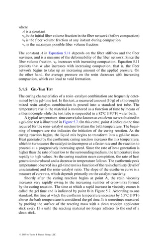
![P4.28. In a drop-weight impact test, a 1 in. diameter spherical ball weighing
0.15 lb is dropped freely on 0.120 in. thick [0=±45=90]3S carbon
fiber–epoxy beam specimens and the rebound heights are recorded.
The beam specimens are simply supported, 0.5 in. wide and 6 in. long
between the supports. The drop heights, rebound heights, and specimen
deflections in three experiments are as follows:
Drop
Height (ft)
Rebound
Height (ft)
Measured Maximum
Deflection (in.)
1 0.72 0.056
4 2.20 0.138
6 3.02 0.150
(a) Calculate the energy lost by the ball in each case.
(b) Assuming that all of the energy lost by the ball is transformed into
strain energy in the beam, calculate the maximum deflection of the
specimen in each case. The flexural modulus of the laminate is 20 3
106
psi.
(c) Explain why the measured maximum deflections are less than those
calculated in (b).
P4.29. The following table* gives the tensile strength and Charpy impact
energy data of a unidirectional hybrid composite containing intermin-
gled carbon and Spectra 1000 polyethylene fibers in an epoxy matrix.
The polyethylene fibers were either untreated or surface-treated to
improve their adhesion with the epoxy matrix. Plot the data as a
function of the polyethylene fiber volume fraction and compare them
with the rule of mixture predictions. Explain the differences in impact
energy in terms of the failure modes that might be expected in untreated
and treated fiber composites. Will you expect differences in other
mechanical properties of these composites?
* A.A.J.M. Peijs, P. Catsman, L.E. Govaert, and P.J. Lemstra, Hybrid composites based on
polyethylene and carbon fibres, Part 2: Influence of composition and adhesion level of polyethylene
fibers on mechanical properties, Composites, 21:513 (1990).
ß 2007 by Taylor Francis Group, LLC.](https://image.slidesharecdn.com/fiberreinforcedcompositesmaterialsmanufacturinganddesignp1-220510152925-9ef3de0d/85/Fiber_Reinforced_Composites_Materials_Manufacturing_and_Design_P-1-pdf-406-320.jpg)
![Polyethylene Fiber
Volume Fraction (%)
Tensile
Strength (MPa)
Charpy Impact
Energy (kJ=m2
)
Untreated Treated Untreated Treated
0 1776 1776 90.8 98.8
20 1623 1666 206 100
40 1367 1384 191 105.1
60 1222 1282 171.2 118.2
80 928 986 140.8 124.8
100 1160 1273 116.7 145.3
P4.30. Show that the time required for a material to attain at least 99.9% of its
maximum possible moisture content is given by
t ¼
0:679c2
Dz
,
where
t is time in seconds
c is the laminate thickness
P4.31. The maximum possible moisture content in a [0=90=±45]S T-300 carbon
fiber–epoxy composite (vf ¼ 0.6) is given by
Mm ¼ 0:000145(RH)1:8
:
A 6.25 mm thick panel of this material is exposed on both sides to air
with 90% relative humidity at 258C. The initial moisture content in the
panel is 0.01%.
(a) Estimate the time required for the moisture content to increase to
the 0.1% level
(b) If the panel is painted on one side with a moisture-impervious
material, what would be the moisture content in the panel at the
end of the time period calculated in (a)?
P4.32. Following Equation 4.43, design an experiment for determining the
diffusion coefficient, Dz of a composite laminate. Be specific about
any calculations that may be required in this experiment.
P4.33. Estimate the transverse tensile strength, transverse modulus, and shear
modulus of a 08 unidirectional T-300 carbon fiber-reinforced epoxy
composite (vf ¼ 0.55) at 508C and 0.1% moisture content. The matrix
ß 2007 by Taylor Francis Group, LLC.](https://image.slidesharecdn.com/fiberreinforcedcompositesmaterialsmanufacturinganddesignp1-220510152925-9ef3de0d/85/Fiber_Reinforced_Composites_Materials_Manufacturing_and_Design_P-1-pdf-407-320.jpg)
![tensile strength, modulus, and Poisson’s ratio at 238C and dry condi-
tions are 56 MPa, 2.2 GPa, and 0.43, respectively; Tgd for the matrix
is 1778C.
P4.34. Shivakumar and Crews* have proposed the following equation for the
bolt clamp-up force Ft between two resin-based laminates:
Ft ¼
F0
1 þ 0:1126(t=ath)0:20
,
where
F0 ¼ initial (elastic) clamp-up force
t ¼ elapsed time (weeks)
ath ¼ a shift factor corresponding to a specific steady-state tempera-
ture or moisture
1. At 238C, the ath values for an epoxy resin are 1, 0.1, 0.01, and 0.001
for 0%, 0.5%, 1%, and 1.5% moisture levels, respectively. Using these
ath values, estimate the time for 20%, 50%, 80%, and 100% relax-
ation in bolt clamp-up force.
2. At 668C and 0.5% moisture level, the bolt clamp-up force relaxes to
80% of its initial value in 3 weeks. Calculate the ath value for this
environmental condition.
P4.35. A quasi-isotropic [0=±45=90]8S panel of T-300 carbon fiber–epoxy
develops a 12 mm long sharp crack at its center. The panel width and
thickness are 200 and 8 mm, respectively. The unnotched tensile
strength of the laminate is 565 MPa. Determine the safe load that can
be applied normal to the crack plane before an unstable fracture occurs.
Describe the possible fracture modes for the cracked panel.
P4.36. The load–displacement record shown in the figure was obtained in a
double-cantilever beam (DCB) test of a unidirectional 08 carbon fiber–
epoxy laminate. The initial crack length was 25 mm and the specimen
was unloaded–reloaded after crack extension of every 5 mm. Plot (a)
compliance vs. crack length and (b) strain energy release rate G1 vs.
crack length for this specimen. What is the Mode I interlaminar fracture
toughness of this material? The specimen width was 25 mm.
* K.N. Shivakumar and J.H. Crews, Jr., Bolt clamp-up relaxation in a graphite=epoxy laminate,
Long-Term Behavior of Composites, ASTM STP, 813:5 (1983).
ß 2007 by Taylor Francis Group, LLC.](https://image.slidesharecdn.com/fiberreinforcedcompositesmaterialsmanufacturinganddesignp1-220510152925-9ef3de0d/85/Fiber_Reinforced_Composites_Materials_Manufacturing_and_Design_P-1-pdf-408-320.jpg)
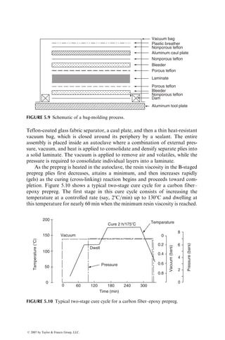
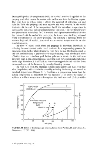
![quality and performance of the molded product. The length of time required to
properly cure a part is called the cure cycle. Since the cure cycle determines the
production rate for a part, it is desirable to achieve the proper cure in the
shortest amount of time. It should be noted that the cure cycle depends on a
number of factors, including resin chemistry, catalyst reactivity, cure tempera-
ture, and the presence of inhibitors or accelerators.
5.1.1 DEGREE OF CURE
A number of investigators [1–3] have experimentally measured the heat evolved
in a curing reaction and related it to the degree of cure achieved at any time
during the curing process. Experiments are performed in a differential scanning
calorimeter (DSC) in which a small sample, weighing a few milligrams, is
heated either isothermally (i.e., at constant temperature) or dynamically (i.e.,
with uniformly increasing temperature). The instrumentation in DSC monitors
the rate of heat generation as a function of time and records it. Figure 5.1
schematically illustrates the rate of heat generation curves for isothermal and
dynamic heating.
The total heat generation to complete a curing reaction (i.e., 100% degree of
cure) is equal to the area under the rate of heat generation–time curve obtained
in a dynamic heating experiment. It is expressed as
HR ¼
ðtf
0
dQ
dt
d
dt, (5:1)
where
HR ¼ heat of reaction
(dQ=dt)d ¼ rate of heat generation in a dynamic experiment
tf ¼ time required to complete the reaction
HR
Rate
of
heat
generation
Rate
of
heat
generation
0
H
(b)
t
Time
0 tf
(a)
Time
FIGURE 5.1 Schematic representation of the rate of heat generation in (a) dynamic and
(b) isothermal heating of a thermoset polymer in a differential scanning calorimeter (DSC).
ß 2007 by Taylor Francis Group, LLC.](https://image.slidesharecdn.com/fiberreinforcedcompositesmaterialsmanufacturinganddesignp1-220510152925-9ef3de0d/85/Fiber_Reinforced_Composites_Materials_Manufacturing_and_Design_P-1-pdf-411-320.jpg)
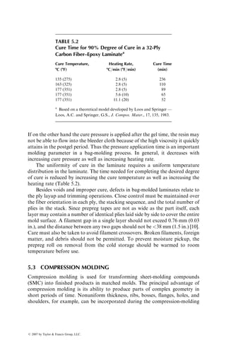
![a maximum value at 10%–40% of the total cure achieved. Higher cure
temperatures increase the rate of cure and produce the maximum degree of
cure in shorter periods of time. On the other hand, the addition of a low-profile
agent, such as a thermoplastic polymer, to a polyester or a vinyl ester resin
decreases the cure rate.
Kamal and Sourour [4] have proposed the following expression for the
isothermal cure rate of a thermoset resin:
dac
dt
¼ (k1 þ k2am
c )(1 ac)n
, (5:4)
where k1 and k2 are reaction rate constants and m and n are constants describ-
ing the order of reaction. The parameters m and n do not vary significantly with
the cure temperature, but k1 and k2 depend strongly on the cure temperature.
With the assumption of a second-order reaction (i.e., m þ n ¼ 2), Equation 5.4
has been used to describe the isothermal cure kinetics of epoxy, unsaturated
polyester, and vinyl ester resins. The values of k1, k2, m, and n are determined
by nonlinear least-squares curve fit to the dac=dt vs. ac data. Typical values of
these constants for a number of resins are listed in Table 5.1.
65⬚C
60⬚C
0.7
0.6
0.5
0.4
0.3
0.2
0.1
0.0
0 0.2 0.4 0.6
Degree of cure (ac)
0.8 1.0
50⬚C
45⬚C
40⬚C
35⬚C
Rate
of
cure
(a
c
)
(per
minute)
FIGURE 5.3 Rate of cure for a vinyl ester resin at various cure temperatures. (After
Han, C.D. and Lem, K.W., J. Appl. Polym. Sci., 29, 1878, 1984.)
ß 2007 by Taylor Francis Group, LLC.](https://image.slidesharecdn.com/fiberreinforcedcompositesmaterialsmanufacturinganddesignp1-220510152925-9ef3de0d/85/Fiber_Reinforced_Composites_Materials_Manufacturing_and_Design_P-1-pdf-413-320.jpg)
![5.1.2 VISCOSITY
Viscosity of a fluid is a measure of its resistance to flow under shear stresses.
Low-molecular-weight fluids, such as water and motor oil, have low viscosities
and flow readily. High-molecular-weight fluids, such as polymer melts, have
high viscosities and flow only under high stresses.
The two most important factors determining the viscosity of a fluid are the
temperature and shear rate. For all fluids, the viscosity decreases with increas-
ing temperature. Shear rate does not have any influence on the viscosity of low-
molecular-weight fluids, whereas it tends to either increase (shear thickening)
or decrease (shear thinning) the viscosity of a high-molecular-weight fluids
(Figure 5.4). Polymer melts, in general, are shear-thinning fluids since their
viscosity decreases with increasing intensity of shearing.
The starting material for a thermoset resin is a low-viscosity fluid. However,
its viscosity increases with curing and approaches a very large value as it
transforms into a solid mass. Variation of viscosity during isothermal curing
of an epoxy resin is shown in Figure 5.5. Similar viscosity–time curves are also
observed for polyester [3] and vinyl ester [5] resins. In all cases, the viscosity
increases with increasing cure time and temperature. The rate of viscosity
increase is low at the early stage of curing. After a threshold degree of cure is
achieved, the resin viscosity increases at a very rapid rate. The time at
which this occurs is called the gel time. The gel time is an important molding
parameter, since the flow of resin in the mold becomes increasingly difficult at
the end of this time period.
A number of important observations can be made from the viscosity data
reported in the literature:
TABLE 5.1
Kinetic Parameters for Various Resin Systems
Resin
Temperature,
8C (8F)
Kinetic Parameters
in Equation 5.4
k1 (per min) k2 (per min) m n
Polyester 45 (113) 0.0131 0.351 0.23 1.77
60 (140) 0.0924 1.57 0.40 1.60
Low-profile polyester
(with 20% polyvinyl
acetate)
45 (113) 0.0084 0.144 0.27 1.73
60 (140) 0.0264 0.282 0.27 1.73
Vinyl ester 45 (113) 0.0073 0.219 0.33 1.76
60 (140) 0.0624 1.59 0.49 1.51
Source: Adapted from Lem, K.W. and Han, C.D., Polym. Eng. Sci., 24, 175, 1984.
ß 2007 by Taylor Francis Group, LLC.](https://image.slidesharecdn.com/fiberreinforcedcompositesmaterialsmanufacturinganddesignp1-220510152925-9ef3de0d/85/Fiber_Reinforced_Composites_Materials_Manufacturing_and_Design_P-1-pdf-414-320.jpg)
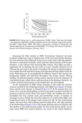
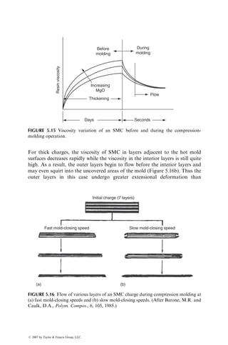
![thermoset polymer is an energy-activated process. Thus, its viscosity as a
function of temperature can be written as
h ¼ ho exp
E
RT
, (5:6)
where
h ¼ viscosity* (Pa s or poise)
E ¼ flow activation energy (cal=g mol)
R ¼ universal gas constant
T ¼ cure temperature (8K)
ho ¼ constant
The activation energy for viscous flow increases with the degree of cure and
approaches a very high value near the gel point.
5.1.3 RESIN FLOW
Proper flow of resin through a dry fiber network (in liquid composite mold-
ing [LCM]) or a prepreg layup (in bag molding) is critical in producing
void-free parts and good fiber wet-out. In thermoset resins, curing may take
place simultaneously with resin flow, and if the resin viscosity rises too rapidly
due to curing, its flow may be inhibited, causing voids and poor interlaminar
adhesion.
Resin flow through fiber network has been modeled using Darcy’s equa-
tion, which was derived for flow of Newtonian fluids through a porous med-
ium. This equation relates the volumetric resin-flow rate q per unit area to the
pressure gradient that causes the flow to occur. For one-dimensional flow in the
x direction,
q ¼
P0
h
dp
dx
, (5:7)
where
q ¼ volumetric flow rate per unit area (m=s) in the x direction
P0 ¼ permeability (m2
)
h ¼ viscosity (N s=m2
)
dp
dx ¼ pressure gradient (N=m3
), which is negative in the direction of flow
(positive x direction)
* Unit of viscosity: 1 Pa s ¼ 1 N s=m2
¼ 10 poise (P) ¼ 1000 centipoise (cP).
ß 2007 by Taylor Francis Group, LLC.](https://image.slidesharecdn.com/fiberreinforcedcompositesmaterialsmanufacturinganddesignp1-220510152925-9ef3de0d/85/Fiber_Reinforced_Composites_Materials_Manufacturing_and_Design_P-1-pdf-417-320.jpg)
![The permeability is determined by the following equation known as the
Kozeny-Carman equation:
P0 ¼
d2
f
16K
(1 vf)3
v2
f
, (5:8)
where
df ¼ fiber diameter
vf ¼ fiber volume fraction
K ¼ Kozeny constant
Equations 5.7 and 5.8, although simplistic, have been used by many investiga-
tors in modeling resin flow from prepregs in bag-molding process and mold
filling in RTM. Equation 5.8 assumes that the porous medium is isotropic, and
the pore size and distribution are uniform. However, fiber networks are non-
isotropic and therefore, the Kozeny constant, K, is not the same in all direc-
tions. For example, for a fiber network with unidirectional fiber orientation,
the Kozeny constant in the transverse direction (K22) is an order of magnitude
higher than the Kozeny constant in the longitudinal direction (K11). This means
that the resin flow in the transverse direction is much lower than that in
the longitudinal direction. Furthermore, the fiber packing in a fiber network
is not uniform, which also affects the Kozeny constant, and therefore the
resin flow.
Equation 5.8 works well for predicting resin flow in the fiber direction.
However, Equation 5.8 is not valid for resin flow in the transverse direction,
since according to this equation resin flow between the fibers does not stop even
when the fiber volume fraction reaches the maximum value at which the fibers
touch each other and there are no gaps between them. Gebart [6] derived the
following permeability equations in the fiber direction and normal to the fiber
direction for unidirectional continuous fiber network with regularly arranged,
parallel fibers.
In the fiber direction: P11 ¼
2d2
f
C1
1 v3
f
v2
f
, (5:9a)
Normal to the fiber direction: P22 ¼ C2
ffiffiffiffiffiffiffiffiffiffiffiffi
vf, max
vf
r
1
5=2
d2
f
4
, (5:9b)
where
C1 ¼ hydraulic radius between the fibers
C2 ¼ a constant
vf,max ¼ maximum fiber volume fraction (i.e., at maximum fiber packing)
ß 2007 by Taylor Francis Group, LLC.](https://image.slidesharecdn.com/fiberreinforcedcompositesmaterialsmanufacturinganddesignp1-220510152925-9ef3de0d/85/Fiber_Reinforced_Composites_Materials_Manufacturing_and_Design_P-1-pdf-418-320.jpg)
![The parameters C1, C2, and vf,max depend on the fiber arrangement in
the network. For a square arrangement of fibers, C1 ¼ 57, C2 ¼ 0.4, and
vf,max ¼ 0.785. For a hexagonal arrangement of fibers (see Problem P2.18),
C1 ¼ 53, C2 ¼ 0.231, and vf,max ¼ 0.906. Note that Equation 5.9a for resin
flow parallel to the fiber direction has the same form as the Kozeny-Carman
equation 5.8. According to Equation 5.9b, which is applicable for resin flow
transverse to the flow direction, P22 ¼ 0 at vf ¼ vf,max, and therefore, the
transverse resin flow stops at the maximum fiber volume fraction.
The permeability equations assume that the fiber distribution is uniform,
the gaps between the fibers are the same throughout the network, the fibers
are perfectly aligned, and all fibers in the network have the same diameter.
These assumptions are not valid in practice, and therefore, the permeability
predictions using Equation 5.8 or 5.9 can only be considered approximate.
5.1.4 CONSOLIDATION
Consolidation of layers in a fiber network or a prepreg layup requires good
resin flow and compaction; otherwise, the resulting composite laminate may
contain a variety of defects, including voids, interply cracks, resin-rich areas, or
resin-poor areas. Good resin flow by itself is not sufficient to produce good
consolidation [7].
Both resin flow and compaction require the application of pressure during
processing in a direction normal to the dry fiber network or prepreg layup. The
pressure is applied to squeeze out the trapped air or volatiles, as the liquid resin
flows through the fiber network or prepreg layup, suppresses voids, and attains
uniform fiber volume fraction. Gutowski et al. [8] developed a model for
consolidation in which it is assumed that the applied pressure is shared by the
fiber network and the resin so that
p ¼ s þ
pr, (5:10)
where
p ¼ applied pressure
s ¼ average effective stress on the fiber network
pr ¼ average pressure on the resin
The average effective pressure on the fiber network increases with increasing
fiber volume fraction and is given by
s ¼ A
1
ffiffiffiffiffi
vf
vo
q
ffiffiffiffiffi
va
vf
q
1
4
, (5:11)
ß 2007 by Taylor Francis Group, LLC.](https://image.slidesharecdn.com/fiberreinforcedcompositesmaterialsmanufacturinganddesignp1-220510152925-9ef3de0d/85/Fiber_Reinforced_Composites_Materials_Manufacturing_and_Design_P-1-pdf-419-320.jpg)
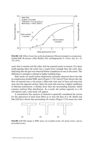
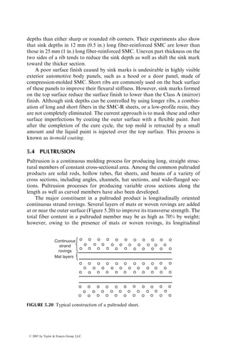
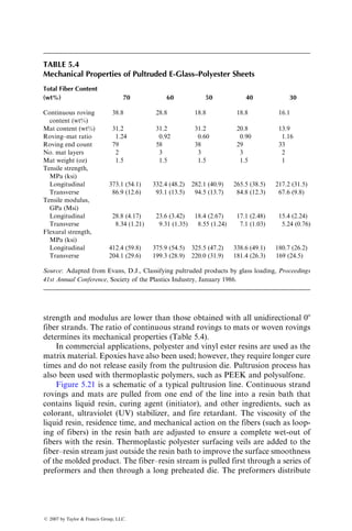
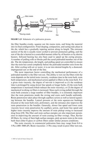
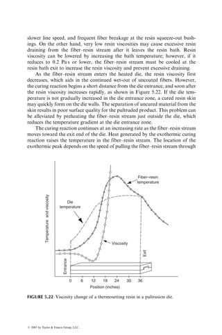
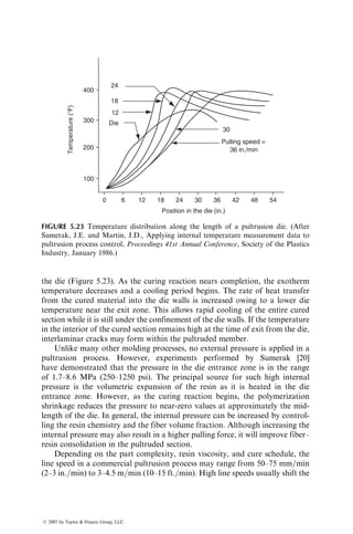
![time for the resin to achieve a low viscosity. A small batch-to-batch variation in
dwell temperature may cause a large variation in gel time, as evidenced in
Figure 5.11.
The cure temperature and pressure are selected to meet the following
requirements:
1. The resin is cured uniformly and attains a specified degree of cure in the
shortest possible time.
2. The temperature at any position inside the prepreg does not exceed a
prescribed limit during the cure.
3. The cure pressure is sufficiently high to squeeze out all of the excess resin
from every ply before the resin gels (increases in viscosity) at any
location inside the prepreg.
Loos and Springer [9] developed a theoretical model for the complex thermo-
mechanical phenomenon that takes place in a vacuum bag-molding process.
Based on their model and experimental works, the following observations can
be made regarding the various molding parameters.
The maximum temperature inside the layup depends on (1) the maximum
cure temperature, (2) the heating rate, and (3) the initial layup thickness. The
maximum cure temperature is usually prescribed by the prepreg manufacturer
for the particular resin–catalyst system used in the prepreg and is determined
from the time–temperature–viscosity characteristics of the resin–catalyst sys-
tem. At low heating rates, the temperature distribution remains uniform within
the layup. At high heating rates and increased layup thickness, the heat gener-
ated by the curing reaction is faster than the heat transferred to the mold
surfaces and a temperature ‘‘overshoot’’ occurs.
Resin flow in the layup depends on the maximum pressure, layup thickness,
and heating rate, as well as the pressure application rate. A cure pressure
sufficient to squeeze out all excess resin from 16 to 32 layups was found to
be inadequate for squeezing out resin from the layers closer to the bottom
surface in a 64-ply layup. Similarly, if the heating rate is very high, the resin
may start to gel before the excess resin is squeezed out from every ply in
the layup.
Loos and Springer [9] have pointed out that the cure cycle recommended by
prepreg manufactures may not be adequate to squeeze out excess resin from
thick layups. Since the compaction and resin flow progress inward from the
top, the plies adjacent to the bottom mold surface may remain uncompacted
and rich in resin, thereby creating weak interlaminar layers in the laminate.
Excess resin must be squeezed out of every ply before the gel point is
reached at any location in the prepreg. Therefore, the maximum cure pressure
should be applied just before the resin viscosity in the top ply becomes suffi-
ciently low for the resin flow to occur. If the cure pressure is applied too early,
excess resin loss would occur owing to very low viscosity in the pregel period.
ß 2007 by Taylor Francis Group, LLC.](https://image.slidesharecdn.com/fiberreinforcedcompositesmaterialsmanufacturinganddesignp1-220510152925-9ef3de0d/85/Fiber_Reinforced_Composites_Materials_Manufacturing_and_Design_P-1-pdf-426-320.jpg)
![If on the other hand the cure pressure is applied after the gel time, the resin may
not be able to flow into the bleeder cloth because of the high viscosity it quickly
attains in the postgel period. Thus the pressure application time is an important
molding parameter in a bag-molding process. In general, it decreases with
increasing cure pressure as well as increasing heating rate.
The uniformity of cure in the laminate requires a uniform temperature
distribution in the laminate. The time needed for completing the desired degree
of cure is reduced by increasing the cure temperature as well as increasing the
heating rate (Table 5.2).
Besides voids and improper cure, defects in bag-molded laminates relate to
the ply layup and trimming operations. Close control must be maintained over
the fiber orientation in each ply, the stacking sequence, and the total number of
plies in the stack. Since prepreg tapes are not as wide as the part itself, each
layer may contain a number of identical plies laid side by side to cover the entire
mold surface. A filament gap in a single layer should not exceed 0.76 mm (0.03
in.), and the distance between any two gaps should not be 38 mm (1.5 in.) [10].
Care must also be taken to avoid filament crossovers. Broken filaments, foreign
matter, and debris should not be permitted. To prevent moisture pickup, the
prepreg roll on removal from the cold storage should be warmed to room
temperature before use.
5.3 COMPRESSION MOLDING
Compression molding is used for transforming sheet-molding compounds
(SMC) into finished products in matched molds. The principal advantage of
compression molding is its ability to produce parts of complex geometry in
short periods of time. Nonuniform thickness, ribs, bosses, flanges, holes, and
shoulders, for example, can be incorporated during the compression-molding
TABLE 5.2
Cure Time for 90% Degree of Cure in a 32-Ply
Carbon Fiber–Epoxy Laminatea
Cure Temperature,
8C (8F)
Heating Rate,
8C=min (8F=min)
Cure Time
(min)
135 (275) 2.8 (5) 236
163 (325) 2.8 (5) 110
177 (351) 2.8 (5) 89
177 (351) 5.6 (10) 65
177 (351) 11.1 (20) 52
a
Based on a theoretical model developed by Loos and Springer —
Loos, A.C. and Springer, G.S., J. Compos. Mater., 17, 135, 1983.
ß 2007 by Taylor Francis Group, LLC.](https://image.slidesharecdn.com/fiberreinforcedcompositesmaterialsmanufacturinganddesignp1-220510152925-9ef3de0d/85/Fiber_Reinforced_Composites_Materials_Manufacturing_and_Design_P-1-pdf-427-320.jpg)
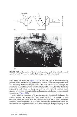
![reasonable degree of cure is achieved under pressure, the mold is opened and
the part is removed, often with the aid of ejector pins.
During molding, a complex heat transfer and a viscous flow phenomenon
take place in the cavity. A review of the current understanding of the flow and
cure characteristics of compression-molded SMC is given in Ref. [11].
Temperature–time curves measured at the outer surface, subsurface, and cen-
terline of thick E-glass fiber-SMC moldings (Figure 5.13) show that the charge
surface temperature quickly attains the mold temperature and remains rela-
tively uniform compared with the centerline temperature. However, owing to
the low thermal conductivity of E-glass fiber-SMC, the centerline temperature
increases slowly until the curing reaction is initiated at the mid-thickness of the
part. Since the SMC material has a relatively low thermal conductivity,
the heat generated by the exothermic curing reaction in the interior of the
SMC charge is not efficiently conducted to the mold surface and the centerline
temperature increases rapidly to a peak value. As the curing reaction nears
completion, the centerline temperature decreases gradually to the mold surface
temperature. For thin parts, the temperature rise is nearly uniform across the
thickness and the maximum temperature in the material seldom exceeds the
mold temperature.
Since the surface temperature first attains the resin gel temperature,
curing begins first at the surface and progresses inward. Curing occurs more
rapidly at higher mold temperatures (Figure 5.14); however, the peak exotherm
temperature may also increase. Since peak exotherm temperature of 2008C or
higher may cause burning and chemical degradation in the resin, high molding
temperatures in thick parts should be avoided.
Temperature
Peak exotherm temperature
Time
Centerline
Mold temperature
Surface
layers
Time to reach reak exotherm
Subsurface layers
FIGURE 5.13 Temperature distribution at various locations across the thickness of an
SMC during the compression-molding operation. (After Mallick, P.K. and Raghupathi,
N., Polym. Eng. Sci., 19, 774, 1979.)
ß 2007 by Taylor Francis Group, LLC.](https://image.slidesharecdn.com/fiberreinforcedcompositesmaterialsmanufacturinganddesignp1-220510152925-9ef3de0d/85/Fiber_Reinforced_Composites_Materials_Manufacturing_and_Design_P-1-pdf-429-320.jpg)
![Increasing the filler content in SMC formulations decreases the peak
exotherm temperature since it replaces part of the resin and thereby decreases
the total amount of heat liberated. It also acts as a heat sink within the material.
The time to reach peak exotherm, which increases almost linearly with the part
thickness, is also reduced with increasing filler content. Thus fillers can play a
significant role in reducing the cure cycle of a part. Another efficient way of
reducing the cure time in the mold is to preheat the charge to pregel temperat-
ures outside the mold and finish curing with high mold-closing speeds inside the
mold. Preheating can be accomplished by dielectric heaters that increase the
temperature rapidly and uniformly throughout the charge volume. During
molding, the thermal gradient remains nearly constant across the thickness of
a preheated charge, which allows uniform curing in the thickness direction. As
a result, residual curing stresses in the molded part are also reduced.
As the temperature of SMC charge increases in the mold, the network
structure created by the thickening reaction with MgO (see Chapter 2) breaks
down and the resin viscosity is reduced (Figure 5.15). If the material does not
attain a low viscosity before gelling, its flow in the mold is severely restricted. If
premature gelation occurs before the mold is filled, the molded part will be
incomplete and may contain voids and interlaminar cracks. A number of
investigators have studied the basic flow behavior of random fiber SMC with
multicolored layers in flat plaque mold cavities [12–14]. At fast mold-closing
speeds, the layers flow with uniform extension (plug flow), with slip occurring
at the mold surface (Figure 5.16a). The charge thickness does not influence this
flow pattern at fast mold-closing speeds. At slow mold-closing speeds, on the
other hand, SMC flow pattern depends very much on the charge thickness.
10
8
6
4
2
0
130 140 150
Mold temperature (⬚C)
Cure
time
(min)
160 175
Thickness (cm)
2.0
1.0
0.25
FIGURE 5.14 Curing time vs. mold temperature of SMC sheets. Note that the shaded
area represents undesirable molding conditions due to the exotherm temperature exceed-
ing 2008C. (After Panter, M.R., The effect to processing variables on curing time and
thermal degradation of compression molded SMC, Proceedings 36th Annual Conference,
Society of the Plastics Industry, February 1981.)
ß 2007 by Taylor Francis Group, LLC.](https://image.slidesharecdn.com/fiberreinforcedcompositesmaterialsmanufacturinganddesignp1-220510152925-9ef3de0d/85/Fiber_Reinforced_Composites_Materials_Manufacturing_and_Design_P-1-pdf-430-320.jpg)
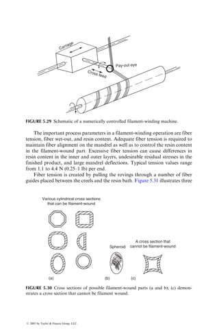
![the interior layers, with slip occurring between the layers as well as at the mold
surface. As the charge thickness is reduced, the extensional deformation
becomes more uniform and approaches the same flow pattern observed at
fast mold-closing speeds. For a good molded part, a rapid mold-closing speed
is desirable since it avoids the possibility of premature gelation and produces
the most uniform flow pattern regardless of the charge thickness [14].
Compression-molded SMC parts may contain a wide variety of surface and
internal defects (Table 5.3). The surface defects usually create a poor surface
appearance or unacceptable surface finish, and the internal defects may affect
performance of the molded part. The origin of some of these defects is discussed
as follows.
Porosity is the result of small internal voids or surface pits (Figure 5.17a)
caused by the entrapment of air or other gases in the molded part. Air is
introduced into the SMC at a number of stages, namely, (1) in the resin paste
during mechanical blending of liquid resin, styrene monomer, and fillers, (2) at
the fiber–resin interface owing to inefficient wetting, (3) in the SMC sheet
during compaction between carrier films, (4) between layers of SMC sheets in
the charge, and (5) in the closed mold. Air entrapped in the SMC before mold
closure is squeezed into small volumes by the pressure exerted during molding.
A substantial amount of these air volumes can be carried away by the material
flowing toward the vents and shear edges. However, if proper venting is not
provided in the mold or the material viscosity is high during its flow, these air
volumes may remain entrapped as voids in the molded part.
Blisters are interlaminar cracks (Figure 5.17b) formed at the end of molding
due to excessive gas pressure in the interior region of the molded part. The
internal gas pressure is generated during molding from unreacted styrene
monomer in undercured parts or from large pockets of entrapped air between
the stacked layers. If this internal pressure is high, interlaminar cracks may form
at the time of mold opening. The delaminated area near the surface may bulge
TABLE 5.3
Common Surface Defects in Compression-Molded SMC
Defect Possible Contributing Factors
Pinhole Coarse filler particles, filler particle agglomeration
Long-range waviness or ripple Resin shrinkage, glass fiber distribution
Craters Poor dispersion of the lubricant (zinc stearate)
Sink marks Resin shrinkage, fiber distribution, fiber length,
fiber orientation
Surface roughness Resin shrinkage, fiber bundle integrity, strand dimensions,
fiber distribution
Dark areas Styrene loss from the surface
Pop-up blisters in painted parts Subsurface voids due to trapped air and volatiles
ß 2007 by Taylor Francis Group, LLC.](https://image.slidesharecdn.com/fiberreinforcedcompositesmaterialsmanufacturinganddesignp1-220510152925-9ef3de0d/85/Fiber_Reinforced_Composites_Materials_Manufacturing_and_Design_P-1-pdf-432-320.jpg)
![into a dome-shaped blister by the entrapped gas pressure. Blisters may also
appear during some postmolding operations, such as high-temperature baking
in a paint oven, which causes expansion of entrapped air or gases.
Griffith and Shanoski [15] suggested two possible ways of reducing blisters:
1. Minimize the entrapped air. The most effective method for minimizing
the entrapped air is vacuum molding, in which air from the mold is
evacuated just as the mold is closed. A second method of reducing the
entrapped air is to allow more radial flow by stacking more plies over a
smaller area instead of stacking fewer plies over a larger area.
2. Increase the interlaminar shear strength by changing the resin type,
using coupling agents, reducing contamination between layers, decreas-
ing the molding temperature, and assuring proper cure before the mold
pressure is released.
In any molding operation involving long flow paths, it is extremely difficult to
control the preferential orientation of fibers. With compression molding of
SMC-R, abrupt changes in thickness, any obstruction in the flow path, or the
Surface
pinholes
Voids
(a)
(c) (d)
(e) (f)
(b)
Fibers oriented
parallel to the edge
Insert
Knit line
Fiber buckling
Blister
Sink mark
Rib
FIGURE 5.17 Various defects in a compression-molded SMC part.
ß 2007 by Taylor Francis Group, LLC.](https://image.slidesharecdn.com/fiberreinforcedcompositesmaterialsmanufacturinganddesignp1-220510152925-9ef3de0d/85/Fiber_Reinforced_Composites_Materials_Manufacturing_and_Design_P-1-pdf-433-320.jpg)
![presence of high shear zones can create fiber orientations that deviate from the
ideal random orientation. As a result, the molded part may become locally
anisotropic with its strength and modulus higher in the direction of flow than
in the transverse direction. In the compression molding of SMC-R, it is common
practice to cover only 60%–70% of the mold surface with the charge, and then use
high normal pressure to spread it over the entire mold cavity. When the flow
front contacts the cavity edges, discontinuous fibers in the SMC-R tend to rotate
normal to the flow direction (Figure 5.17c). This results in strength reduction
normal to the flow direction and makes the edges prone to early cracking.
Compression molding of SMC-CR or XMC containing continuous fibers is
normally performed with 90%–95% initial mold surface coverage. For these
materials, flow is possible only in the transverse direction of fibers. If excessive
transverse flow is allowed, continuous fibers in the surface and subsurface
layers of both SMC-CR and XMC may buckle (bow out) near the end of the
flow path (Figure 5.17d). In addition, the included angle between the
X-patterned fibers in XMC may also increase. As a result, the longitudinal
tensile strengths of SMC-CR and XMC are reduced in areas with fiber mis-
orientation [16]. However, since severe fiber misorientations are generally
restricted to the outer layers, increasing the number of plies improves the
longitudinal strength to the level observed with no misorientation.
Knit lines are linear domains of aligned fiber orientation and are formed at
the joining of two divided flow fronts (Figure 5.17e), such as behind a metal
insert or pin or where two or more separate flow fronts arising from multiple
charge pieces meet. Multiple charge pieces are used for compression molding of
large and complex parts. Since fibers tend to align themselves along the knit
line, the strength of the part in a direction normal to the knit line is reduced.
The formation of knit lines can be reduced by proper charge placement in
the mold. A common location of knit lines in behind a core pin used in forming
molded-in holes. Thus if the holes are in a high-stress area, it is better to drill
them instead of using core pins, since knit lines formed behind such core pins
may extend to the edge and initiate premature cracking.
Warpage is critical in thin-section moldings and is caused by variations in
cooling rate between sections of different thicknesses or different fiber orien-
tations. Differential cooling rates may also lead to complex residual stresses,
which may ultimately reduce the strength of a molded part.
Nonuniform cure is critical in thick-section moldings and can create a
gradient of properties in the thickness direction. Since the curing reaction is
initiated at the surfaces and progresses inward, it is likely that insufficient
molding time will leave the interior undercured. As a result, the interlaminar
shear strength of the molded part is reduced.
The effect of various molding times on the development of through-
thickness properties of a thick-section molding is demonstrated in Figure 5.18.
This figure was developed by sectioning 12 mm (0.5 in.) thick compression-molded
specimens along the center plane and testing each half in flexure, one with the
ß 2007 by Taylor Francis Group, LLC.](https://image.slidesharecdn.com/fiberreinforcedcompositesmaterialsmanufacturinganddesignp1-220510152925-9ef3de0d/85/Fiber_Reinforced_Composites_Materials_Manufacturing_and_Design_P-1-pdf-434-320.jpg)
![outer skin in tension and the other with the exposed center in tension. For short
mold-opening times the center has a much lower strength than the outer skin,
indicating that the part was removed before completion of cure at the center. The
difference in strength is reduced at higher molding times.
Sink marks are small surface depressions normally observed above the ribs
in compression-molded SMC parts (Figure 5.17f). Jutte [17] has shown that the
flow of material into a rib creates a fiber-rich zone near its base and resin-rich
zone near the opposite surface. Since the resin-rich zone has a higher coefficient
of thermal contraction, it shrinks more than the surrounding material, which
contains uniform fiber distribution. As a result, the surface opposite to a rib
will depress and a sink mark will appear.
A nonuniform flow pattern of material is generally considered the reason
for the separation of resin from fibers at or near the base of a rib. Smith and
Suh [18] have shown that protruding rib corners (Figure 5.19) create less sink
40
35
30
2 3 4 5
Mold-opening time (min)
Center section
in tension
Outer surface
in tension
SMC-R50
Thickness=12.7 cm (0.5 in.)
Mold temp.=1498C (300⬚F)
E-glass–vinyl ester
6 7
276
207
Flexural
strength
(MPa)
Flexural
strength
(ksi)
FIGURE 5.18 Effect of cure time on the development of flexural strength in a compression-
molded SMC-R laminate. (After Mallick, P.K. and Raghupathi, N., Polym. Eng. Sci., 19,
774, 1979.)
(a) (b) (c)
FIGURE 5.19 Rib design in SMC parts: (a) rounded corner, (b) sharp corner, and (c)
protruded corner.
ß 2007 by Taylor Francis Group, LLC.](https://image.slidesharecdn.com/fiberreinforcedcompositesmaterialsmanufacturinganddesignp1-220510152925-9ef3de0d/85/Fiber_Reinforced_Composites_Materials_Manufacturing_and_Design_P-1-pdf-435-320.jpg)
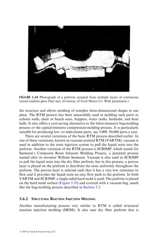
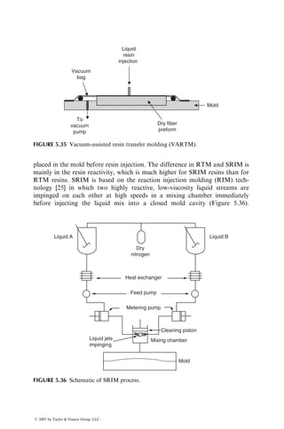
![the fiber bundles evenly, squeeze out the excess resin, and bring the material
into its final configuration. Final shaping, compaction, and curing take place in
the die, which has a gradually tapering section along its length. The entrance
section of the die is usually water cooled to prevent premature gelling, and the
rest of the die is heated in a controlled manner either by oil heaters or by electric
heaters. Infrared heating has also been used to speed up the curing process.
A number of pulling rolls or blocks pull the cured pultruded member out of the
die. The die temperature, die length, and pulling speed are controlled to ensure
that the resin has cured completely before the pultruded member exits from the
die. After cooling with air or water, it is cut into desired lengths by a diamond-
impregnated saw at the end of the line.
The most important factor controlling the mechanical performance of a
pultruded member is the fiber wet-out. The ability to wet out the fibers with the
resin depends on the initial resin viscosity, residence time in the resin bath, resin
bath temperature, and mechanical action applied to fibers in the resin bath. For
a given resin viscosity, the degree of wet-out is improved as (1) the residence
time is prolonged by using slower line speeds or longer baths, (2) the resin bath
temperature is increased (which reduces the resin viscosity), or (3) the degree of
mechanical working on fibers is increased. Since each roving pulled through the
resin bath contains a large number of fiber bundles, it is extremely important
that the resin penetrates inside the roving and coats each bundle uniformly.
Resin penetration takes place through capillary action as well as lateral squeez-
ing between the bundles. Lateral pressure at the resin squeeze-out bushings
(located at the resin bath exit), preformers, and die entrance also improves the
resin penetration in the bundles. Generally, slower line speed and lower resin
viscosity favor resin penetration by capillary action, and faster line speed and
higher resin viscosity improve the amount of resin pickup owing to increased
drag force [19]. The fiber and resin surface energies are also important param-
eters in improving the amount of resin coating on fiber rovings. Thus, Kevlar
49 fibers, by virtue of their high surface energies, pick up more resin in the resin
bath than either E-glass or carbon fibers under similar process conditions.
The resin viscosity in commercial pultrusion lines may range from 0.4 to
5 Pa s (400–5000 cP). Resin viscosities 5 Pa s may result in poor fiber wet-out,
Mat creels
Resin bath
Surfacing veil Cut-off
saw
Guide
Roving creels
Preformer
Die
Pull blocks
FIGURE 5.21 Schematic of a pultrusion process.
ß 2007 by Taylor Francis Group, LLC.](https://image.slidesharecdn.com/fiberreinforcedcompositesmaterialsmanufacturinganddesignp1-220510152925-9ef3de0d/85/Fiber_Reinforced_Composites_Materials_Manufacturing_and_Design_P-1-pdf-438-320.jpg)
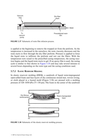
![the die (Figure 5.23). As the curing reaction nears completion, the exotherm
temperature decreases and a cooling period begins. The rate of heat transfer
from the cured material into the die walls is increased owing to a lower die
temperature near the exit zone. This allows rapid cooling of the entire cured
section while it is still under the confinement of the die walls. If the temperature
in the interior of the cured section remains high at the time of exit from the die,
interlaminar cracks may form within the pultruded member.
Unlike many other molding processes, no external pressure is applied in a
pultrusion process. However, experiments performed by Sumerak [20]
have demonstrated that the pressure in the die entrance zone is in the range
of 1.7–8.6 MPa (250–1250 psi). The principal source for such high internal
pressure is the volumetric expansion of the resin as it is heated in the die
entrance zone. However, as the curing reaction begins, the polymerization
shrinkage reduces the pressure to near-zero values at approximately the mid-
length of the die. In general, the internal pressure can be increased by control-
ling the resin chemistry and the fiber volume fraction. Although increasing the
internal pressure may also result in a higher pulling force, it will improve fiber–
resin consolidation in the pultruded section.
Depending on the part complexity, resin viscosity, and cure schedule, the
line speed in a commercial pultrusion process may range from 50–75 mm=min
(2–3 in.=min) to 3–4.5 m=min (10–15 ft.=min). High line speeds usually shift the
24
18
12
Die
30
Pulling speed =
36 in./min
Position in the die (in.)
0 6 12 18 24 30 36 42 48 54
100
200
300
400
Temperature
(⬚F)
FIGURE 5.23 Temperature distribution along the length of a pultrusion die. (After
Sumerak, J.E. and Martin, J.D., Applying internal temperature measurement data to
pultrusion process control, Proceedings 41st Annual Conference, Society of the Plastics
Industry, January 1986.)
ß 2007 by Taylor Francis Group, LLC.](https://image.slidesharecdn.com/fiberreinforcedcompositesmaterialsmanufacturinganddesignp1-220510152925-9ef3de0d/85/Fiber_Reinforced_Composites_Materials_Manufacturing_and_Design_P-1-pdf-440-320.jpg)
![location of the peak exotherm temperature toward the exit end of the die and
increase the pulling force. Although the production rate is increased at high line
speeds, the product quality may deteriorate owing to poor fiber wet-out,
unfinished curing, and roving migration within the cross section. If high output
is desired, it is often better to use multiple dies instead of high line speeds.
The pulling force applied to the pulling mechanism at the end of the pultru-
sion line must overcome the combined effects of (1) the frictional force of fibers
sliding against the die wall, (2) the shear viscous force between a very thin layer
of resin and the die wall, and (3) the backflow force or drag resistance between
the fibers and the backflowing resin at the die entrance. The contribution from
each of these forces to the total pulling force varies along the length of the die.
For example, the shear viscous force and the backflow force have larger contri-
butions near the die entrance. As curing progresses along the die length and the
liquid resin transforms into a solid mass, the frictional force becomes more
predominant. The theoretical model developed by Bibbo and Gutowski [21]
shows that the pulling force increases with increasing fiber volume fraction,
resin viscosity, line speed, and compaction ratio (i.e., the ratio of the die
entrance opening to the die exit opening). However, contributions from each
of these parameters on the frictional force, shear viscous force, and backflow
force are not uniform. Control of the pulling force and the design of the fiber
guidance system are extremely important since they influence the fiber align-
ment as well as fiber wet-out. Some of the defects found in pultruded products,
such as fiber bunching, fiber shifting, wrinkles, and folding of mats or woven
rovings, are related to these factors.
5.5 FILAMENT WINDING
In a filament-winding process, a band of continuous resin-impregnated rovings
or monofilaments is wrapped around a rotating mandrel and cured to produce
axisymmetric hollow parts. Among the applications of filament winding are
automotive drive shafts, helicopter blades, oxygen tanks, pipelines, spherical
pressure vessels, conical rocket motor cases, and large underground gasoline
storage tanks. The filament-winding process is also used to manufacture prepreg
sheets or continuous fiber-reinforced sheet-molding compounds, such as XMC.
The sheet is formed by slitting the wound shape parallel to the mandrel axis.
Figure 5.24 shows the schematic of a basic filament-winding process.
A large number of fiber rovings are pulled from a series of creels into a liquid
resin bath containing liquid resin, catalyst, and other ingredients, such as
pigments and UV absorbers. Fiber tension is controlled using the fiber guides
or scissor bars located between each creel and the resin bath. Just before
entering the resin bath, the rovings are usually gathered into a band by passing
them through a textile thread board or a stainless steel comb.
At the end of the resin tank, the resin-impregnated rovings are pulled
through a wiping device that removes the excess resin from the rovings and
ß 2007 by Taylor Francis Group, LLC.](https://image.slidesharecdn.com/fiberreinforcedcompositesmaterialsmanufacturinganddesignp1-220510152925-9ef3de0d/85/Fiber_Reinforced_Composites_Materials_Manufacturing_and_Design_P-1-pdf-441-320.jpg)
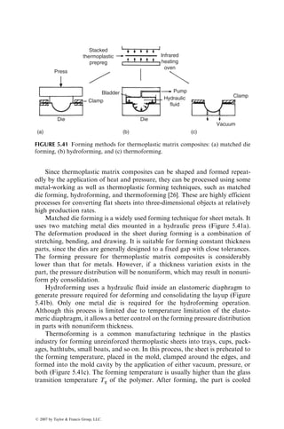
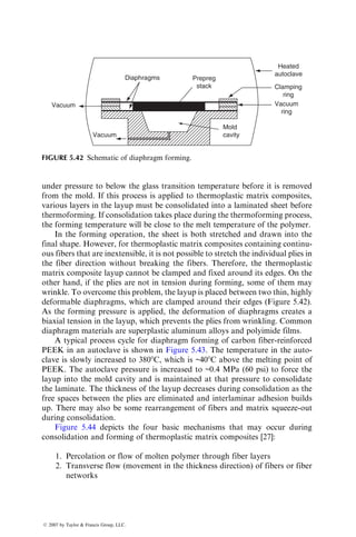
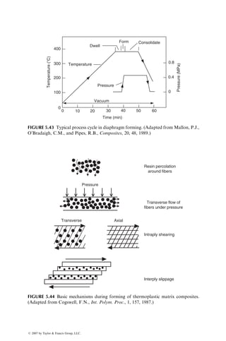
![circular mandrel rotating with a constant rotational speed of N revolutions per
minute and a constant carriage feed of V, the wind angle is given by
u ¼
2pNr
V
, (5:12)
where r is the radius of the mandrel. Equation 5.12 shows that a constant wind
angle can be maintained in a thick part only if the ratio N=V is adjusted from
layer to layer. Winding with the conventional machine also requires the
carriage to travel extra lengths on both sides of the mandrel.
The versatility of filament-winding process is improved tremendously if
numerical controls are added to the filament-winding machine [22,23]. In
numerically controlled machines, independent drives are used for the mandrel
as well as for the carriage. In addition, a cross (transverse) feed mechanism and
a rotating pay-out eye (Figure 5.29) allow an unequal fiber placement on the
mandrel. The cross feed mechanism is mounted on the carriage and can move in
and out radially; the pay-out eye can be controlled to rotate about a horizontal
axis. The combination of these two motions prevents fiber slippage as well as
fiber bunching on mandrels of irregular shape. Although each mechanism is
driven by its own hydraulic motor, their movements are related to the mandrel
rotation by numerical controls. Since no mechanical connections are involved,
wind angles can be varied without much manual operation. With conventional
filament-winding machines, the shapes that can be created are limited to
surfaces of revolution, such as cylinders of various cross sections, cones, box
beams, or spheroids (Figure 5.30). The computer-controlled multiaxis machines
can wind irregular and complex shapes with no axis of symmetry, such as the
aerodynamic shape of a helicopter blade.
Head
stock
and
control
gear
box
Sprocket
Spindle
Mandrel
Carriage
Tail
stock
Secondary chain drive
Primary
chain drive
FIGURE 5.28 Schematic of a conventional filament-winding machine.
ß 2007 by Taylor Francis Group, LLC.](https://image.slidesharecdn.com/fiberreinforcedcompositesmaterialsmanufacturinganddesignp1-220510152925-9ef3de0d/85/Fiber_Reinforced_Composites_Materials_Manufacturing_and_Design_P-1-pdf-445-320.jpg)
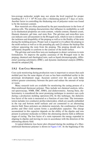
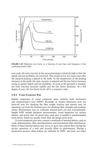
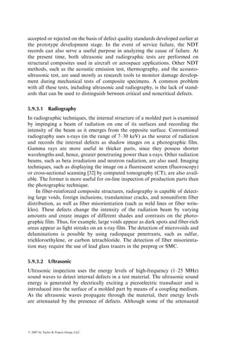
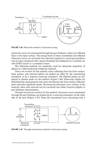
![continuous fiber rovings, are sprayed onto a preshaped screen. Vacuum applied
to the rear side of the screen holds the fibers securely on the screen. A binder
sprayed with the fibers keeps them in place and maintains the preformed shape.
Continuous strand mats containing random fibers can be preformed by a
stamping operation using a simple press and a preshaped die (Figure 5.34).
Both thermoplastic and thermoset binders are available for retaining the
formed shape after stamping. With woven fabric containing bidirectional
fibers, a ‘‘cut and sew’’ method is used in which various patterns are first cut
from the fabric and then stitched together by polyester, glass, or Kevlar sewing
threads into the shape of the part that is being produced. Braiding and textile
weaving processes have also been used to produce two- or three-dimensional
preforms [24]. Braiding is particularly suitable for producing tubular preforms.
Compared with the compression-molding process, RTM has a very low
tooling cost and simple mold clamping requirements. In some cases, a ratchet
clamp or a series of nuts and bolts can be used to hold the two mold halves
together. RTM is a low-pressure process, and therefore parts can be resin
transfer molded in low-tonnage presses. A second advantage of the RTM
process is its ability to encapsulate metal inserts, stiffeners, washers, and so
on within the molded laminate. It is also possible to encapsulate a foam core
between the top and bottom preforms of a hollow part, which adds stiffness to
Fiber mat
rolls
Preforms made
in a preform press
Foam
Preforms placed in the
mold with foam core in
this example
Mold closed and
liquid resin injected
Molded part
FIGURE 5.33 Schematic of RTM process.
ß 2007 by Taylor Francis Group, LLC.](https://image.slidesharecdn.com/fiberreinforcedcompositesmaterialsmanufacturinganddesignp1-220510152925-9ef3de0d/85/Fiber_Reinforced_Composites_Materials_Manufacturing_and_Design_P-1-pdf-450-320.jpg)
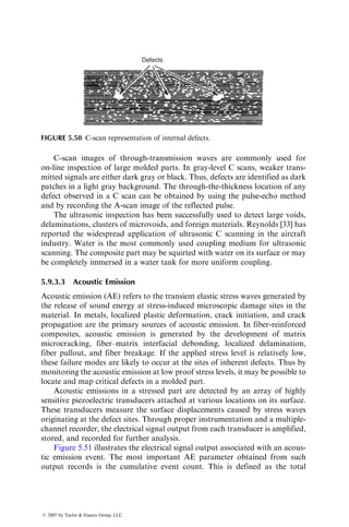
![placed in the mold before resin injection. The difference in RTM and SRIM is
mainly in the resin reactivity, which is much higher for SRIM resins than for
RTM resins. SRIM is based on the reaction injection molding (RIM) tech-
nology [25] in which two highly reactive, low-viscosity liquid streams are
impinged on each other at high speeds in a mixing chamber immediately
before injecting the liquid mix into a closed mold cavity (Figure 5.36).
Dry fiber
preform
Liquid
resin
injection
Mold
To
vacuum
pump
Vacuum
bag
FIGURE 5.35 Vacuum-assisted resin transfer molding (VARTM).
Liquid A
Dry
nitrogen
Heat exchanger
Feed pump
Metering pump
Cleaning piston
Mixing chamber
Mold
Liquid jets
impinging
Liquid B
FIGURE 5.36 Schematic of SRIM process.
ß 2007 by Taylor Francis Group, LLC.](https://image.slidesharecdn.com/fiberreinforcedcompositesmaterialsmanufacturinganddesignp1-220510152925-9ef3de0d/85/Fiber_Reinforced_Composites_Materials_Manufacturing_and_Design_P-1-pdf-452-320.jpg)
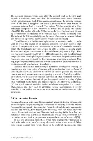
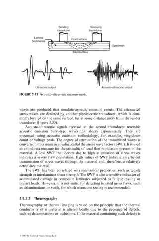
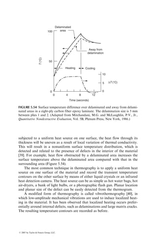
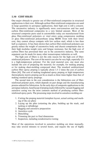
![Since thermoplastic matrix composites can be shaped and formed repeat-
edly by the application of heat and pressure, they can be processed using some
metal-working as well as thermoplastic forming techniques, such as matched
die forming, hydroforming, and thermoforming [26]. These are highly efficient
processes for converting flat sheets into three-dimensional objects at relatively
high production rates.
Matched die forming is a widely used forming technique for sheet metals. It
uses two matching metal dies mounted in a hydraulic press (Figure 5.41a).
The deformation produced in the sheet during forming is a combination of
stretching, bending, and drawing. It is suitable for forming constant thickness
parts, since the dies are generally designed to a fixed gap with close tolerances.
The forming pressure for thermoplastic matrix composites is considerably
lower than that for metals. However, if a thickness variation exists in the
part, the pressure distribution will be nonuniform, which may result in nonuni-
form ply consolidation.
Hydroforming uses a hydraulic fluid inside an elastomeric diaphragm to
generate pressure required for deforming and consolidating the layup (Figure
5.41b). Only one metal die is required for the hydroforming operation.
Although this process is limited due to temperature limitation of the elasto-
meric diaphragm, it allows a better control on the forming pressure distribution
in parts with nonuniform thickness.
Thermoforming is a common manufacturing technique in the plastics
industry for forming unreinforced thermoplastic sheets into trays, cups, pack-
ages, bathtubs, small boats, and so on. In this process, the sheet is preheated to
the forming temperature, placed in the mold, clamped around the edges, and
formed into the mold cavity by the application of either vacuum, pressure, or
both (Figure 5.41c). The forming temperature is usually higher than the glass
transition temperature Tg of the polymer. After forming, the part is cooled
Stacked
thermoplastic
prepreg
Clamp
Bladder
Hydraulic
fluid
Pump
Clamp
Vacuum
Press
Die
(b) (c)
(a)
Die
Infrared
heating
oven
FIGURE 5.41 Forming methods for thermoplastic matrix composites: (a) matched die
forming, (b) hydroforming, and (c) thermoforming.
ß 2007 by Taylor Francis Group, LLC.](https://image.slidesharecdn.com/fiberreinforcedcompositesmaterialsmanufacturinganddesignp1-220510152925-9ef3de0d/85/Fiber_Reinforced_Composites_Materials_Manufacturing_and_Design_P-1-pdf-457-320.jpg)
![under pressure to below the glass transition temperature before it is removed
from the mold. If this process is applied to thermoplastic matrix composites,
various layers in the layup must be consolidated into a laminated sheet before
thermoforming. If consolidation takes place during the thermoforming process,
the forming temperature will be close to the melt temperature of the polymer.
In the forming operation, the sheet is both stretched and drawn into the
final shape. However, for thermoplastic matrix composites containing continu-
ous fibers that are inextensible, it is not possible to stretch the individual plies in
the fiber direction without breaking the fibers. Therefore, the thermoplastic
matrix composite layup cannot be clamped and fixed around its edges. On the
other hand, if the plies are not in tension during forming, some of them may
wrinkle. To overcome this problem, the layup is placed between two thin, highly
deformable diaphragms, which are clamped around their edges (Figure 5.42).
As the forming pressure is applied, the deformation of diaphragms creates a
biaxial tension in the layup, which prevents the plies from wrinkling. Common
diaphragm materials are superplastic aluminum alloys and polyimide films.
A typical process cycle for diaphragm forming of carbon fiber-reinforced
PEEK in an autoclave is shown in Figure 5.43. The temperature in the auto-
clave is slowly increased to 3808C, which is ~408C above the melting point of
PEEK. The autoclave pressure is increased to ~0.4 MPa (60 psi) to force the
layup into the mold cavity and is maintained at that pressure to consolidate
the laminate. The thickness of the layup decreases during consolidation as the
free spaces between the plies are eliminated and interlaminar adhesion builds
up. There may also be some rearrangement of fibers and matrix squeeze-out
during consolidation.
Figure 5.44 depicts the four basic mechanisms that may occur during
consolidation and forming of thermoplastic matrix composites [27]:
1. Percolation or flow of molten polymer through fiber layers
2. Transverse flow (movement in the thickness direction) of fibers or fiber
networks
Heated
autoclave
Clamping
ring
Vacuum
ring
Mold
cavity
Prepreg
stack
Diaphragms
Vacuum
Vacuum
FIGURE 5.42 Schematic of diaphragm forming.
ß 2007 by Taylor Francis Group, LLC.](https://image.slidesharecdn.com/fiberreinforcedcompositesmaterialsmanufacturinganddesignp1-220510152925-9ef3de0d/85/Fiber_Reinforced_Composites_Materials_Manufacturing_and_Design_P-1-pdf-458-320.jpg)
![3. Intraply shearing which allows fibers within each ply to move relative to
each other in the axial as well as in the transverse direction
4. Interply slip, by which plies slide over each other while conforming to
the shape of the die
The first two mechanisms are essential for good consolidation, since they help
reduce the gaps and voids that exist between the plies as well as within each ply
and create good interlaminar adhesion. The other two mechanisms help in
forming contoured shapes without fiber wrinkling, splitting, or local thinning.
5.9 QUALITY INSPECTION METHODS
The mechanical properties of a molded part and their variations from part to
part depend on many factors, including the quality of raw materials, the degree
of cure, and the presence of molding defects in the part. Many of the molding
defects can be either eliminated or reduced by proper part and mold designs as
well as by controlling the various process parameters described in the earlier
sections. Since complete elimination of all molding defects is not possible, it is
important that the quality of the molded parts be inspected regularly for critical
defects that can cause premature failure in a part during its service. The
criticality of a defect or a group of defects is established through extensive
testing at the prototype development stage. The quality inspection techniques
and the part acceptance criteria are also established at the prototype develop-
ment stage.
5.9.1 RAW MATERIALS
Among the raw materials, the two most important candidates for close quality
inspection are fibers and resin. Measurements of tensile strength and modulus
are the primary screening methods for continuous fibers. For the resin, curing
agents, or diluents, the standard quality inspection items are the density,
viscosity, color, and moisture content. Additional tests recommended for the
incoming resin and other components [28] are (1) wet chemical analysis to
determine the amount of functional groups (such as epoxide groups in epoxies
or acid numbers in polyesters) in the material, (2) infrared (IR) spectroscopy or
nuclear magnetic resonance (NMR) spectroscopy to fingerprint the chemical
structure and impurities, and (3) liquid chromatography or gel permeation
chromatography (GPC) to determine the weight-average molecular weight
and molecular weight distribution of the resin molecules.
The average molecular weight and molecular weight distribution are
two very important characteristics of a resin that control its viscosity and
mechanical properties. Burns et al. [29] have shown that high fractions of
low-molecular-weight molecules in a polyester resin reduce the rate of thicken-
ing (viscosity increase) in SMC sheets. The viscosity of a polyester resin with
ß 2007 by Taylor Francis Group, LLC.](https://image.slidesharecdn.com/fiberreinforcedcompositesmaterialsmanufacturinganddesignp1-220510152925-9ef3de0d/85/Fiber_Reinforced_Composites_Materials_Manufacturing_and_Design_P-1-pdf-460-320.jpg)
![low-average molecular weight may not attain the level required for proper
handling (0.5–1.3 3 106
P) even after a thickening period of 7 days or more.
Another factor in controlling the thickening rate of polyester resins was found
to be the moisture content.
Raw materials are often purchased by the part manufacturer in the form of
prepreg rolls. The prepreg characteristics that influence its moldability as well
as its mechanical properties are resin content, volatile content, filament count,
filament diameter, gel time, and resin flow. The gel-time and resin-flow tests
can indicate cure advancement in the B-staged resin, which in turn is related to
the tackiness and drapability of the prepreg as well as to the fluidity of the resin
during the molding process. Proper tack is required to (1) adhere the prepreg to
the mold surface as well as to the preceding ply and (2) release the backup film
without separating the resin from the prepreg. The prepreg should also be
sufficiently drapable to conform to the contour of the mold surface.
The gel-time and resin-flow tests are inadequate to detect variations in resin
formulation. To improve the quality assurance of the B-staged resin in the
prepreg, chemical and rheological tests, such as liquid chromatography, differ-
ential scanning calorimetry (DSC), and dynamic mechanical analysis (DMA),
should be adopted [30].
5.9.2 CURE CYCLE MONITORING
Cure cycle monitoring during production runs is important to ensure that each
molded part has the same degree of cure as has been established earlier in the
prototype development stage. Accurate control over the cure cycle helps
achieve greater consistency between the parts and reduce the amount of scrap
or waste.
Many research tools are available for monitoring the curing process of a
fiber-reinforced thermoset polymer. They include wet chemical analysis, infra-
red spectroscopy, NMR, DSC, DMA, and dielectrometry. Among these, die-
lectrometry is considered the most promising technique to monitor cure cycle
during a production molding operation [31]. In this technique, the dielectric
loss factor of the resin is measured as a function of cure time. The instrumen-
tation includes two conductor probes (electrodes), which are usually embedded
in the top and bottom mold surfaces and are connected to an alternating
electric field. Since polymers are dielectric materials, the combination of these
probes and fiber–resin system forms a parallel-plate capacitor. The charge
accumulated in this capacitor depends on the ability of the dipoles and ions
present in polymer molecules to follow the alternating electric field at different
stages of curing. The loss factor of a resin represents the energy expended in
aligning its dipoles and moving its ions in accordance with the direction of the
alternating electric field.
A typical dielectric loss factor plot obtained during the molding of a fiber-
reinforced thermoset polymer is shown in Figure 5.45. At the beginning of the
ß 2007 by Taylor Francis Group, LLC.](https://image.slidesharecdn.com/fiberreinforcedcompositesmaterialsmanufacturinganddesignp1-220510152925-9ef3de0d/85/Fiber_Reinforced_Composites_Materials_Manufacturing_and_Design_P-1-pdf-461-320.jpg)
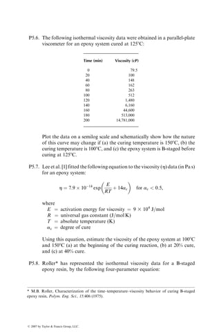
![accepted or rejected on the basis of defect quality standards developed earlier at
the prototype development stage. In the event of service failure, the NDT
records can also serve a useful purpose in analyzing the cause of failure. At
the present time, both ultrasonic and radiographic tests are performed on
structural composites used in aircraft or aerospace applications. Other NDT
methods, such as the acoustic emission test, thermography, and the acousto-
ultrasonic test, are used mostly as research tools to monitor damage develop-
ment during mechanical tests of composite specimens. A common problem
with all these tests, including ultrasonic and radiography, is the lack of stand-
ards that can be used to distinguish between critical and noncritical defects.
5.9.3.1 Radiography
In radiographic techniques, the internal structure of a molded part is examined
by impinging a beam of radiation on one of its surfaces and recording the
intensity of the beam as it emerges from the opposite surface. Conventional
radiography uses x-rays (in the range of 7–30 keV) as the source of radiation
and records the internal defects as shadow images on a photographic film.
Gamma rays are more useful in thicker parts, since they possess shorter
wavelengths and, hence, greater penetrating power than x-rays. Other radiation
beams, such as beta irradiation and neutron radiation, are also used. Imaging
techniques, such as displaying the image on a fluorescent screen (fluoroscopy)
or cross-sectional scanning [32] by computed tomography (CT), are also avail-
able. The former is more useful for on-line inspection of production parts than
the photographic technique.
In fiber-reinforced composite structures, radiography is capable of detect-
ing large voids, foreign inclusions, translaminar cracks, and nonuniform fiber
distribution, as well as fiber misorientation (such as weld lines or fiber wrin-
kles). These defects change the intensity of the radiation beam by varying
amounts and create images of different shades and contrasts on the photo-
graphic film. Thus, for example, large voids appear as dark spots and fiber-rich
areas appear as light streaks on an x-ray film. The detection of microvoids and
delaminations is possible by using radiopaque penetrants, such as sulfur,
trichloroethylene, or carbon tetrachloride. The detection of fiber misorienta-
tion may require the use of lead glass tracers in the prepreg or SMC.
5.9.3.2 Ultrasonic
Ultrasonic inspection uses the energy levels of high-frequency (1–25 MHz)
sound waves to detect internal defects in a test material. The ultrasonic sound
energy is generated by electrically exciting a piezoelectric transducer and is
introduced into the surface of a molded part by means of a coupling medium.
As the ultrasonic waves propagate through the material, their energy levels
are attenuated by the presence of defects. Although some of the attenuated
ß 2007 by Taylor Francis Group, LLC.](https://image.slidesharecdn.com/fiberreinforcedcompositesmaterialsmanufacturinganddesignp1-220510152925-9ef3de0d/85/Fiber_Reinforced_Composites_Materials_Manufacturing_and_Design_P-1-pdf-463-320.jpg)
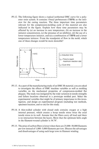
![C-scan images of through-transmission waves are commonly used for
on-line inspection of large molded parts. In gray-level C scans, weaker trans-
mitted signals are either dark gray or black. Thus, defects are identified as dark
patches in a light gray background. The through-the-thickness location of any
defect observed in a C scan can be obtained by using the pulse-echo method
and by recording the A-scan image of the reflected pulse.
The ultrasonic inspection has been successfully used to detect large voids,
delaminations, clusters of microvoids, and foreign materials. Reynolds [33] has
reported the widespread application of ultrasonic C scanning in the aircraft
industry. Water is the most commonly used coupling medium for ultrasonic
scanning. The composite part may be squirted with water on its surface or may
be completely immersed in a water tank for more uniform coupling.
5.9.3.3 Acoustic Emission
Acoustic emission (AE) refers to the transient elastic stress waves generated by
the release of sound energy at stress-induced microscopic damage sites in the
material. In metals, localized plastic deformation, crack initiation, and crack
propagation are the primary sources of acoustic emission. In fiber-reinforced
composites, acoustic emission is generated by the development of matrix
microcracking, fiber–matrix interfacial debonding, localized delamination,
fiber pullout, and fiber breakage. If the applied stress level is relatively low,
these failure modes are likely to occur at the sites of inherent defects. Thus by
monitoring the acoustic emission at low proof stress levels, it may be possible to
locate and map critical defects in a molded part.
Acoustic emissions in a stressed part are detected by an array of highly
sensitive piezoelectric transducers attached at various locations on its surface.
These transducers measure the surface displacements caused by stress waves
originating at the defect sites. Through proper instrumentation and a multiple-
channel recorder, the electrical signal output from each transducer is amplified,
stored, and recorded for further analysis.
Figure 5.51 illustrates the electrical signal output associated with an acous-
tic emission event. The most important AE parameter obtained from such
output records is the cumulative event count. This is defined as the total
Defects
FIGURE 5.50 C-scan representation of internal defects.
ß 2007 by Taylor Francis Group, LLC.](https://image.slidesharecdn.com/fiberreinforcedcompositesmaterialsmanufacturinganddesignp1-220510152925-9ef3de0d/85/Fiber_Reinforced_Composites_Materials_Manufacturing_and_Design_P-1-pdf-466-320.jpg)
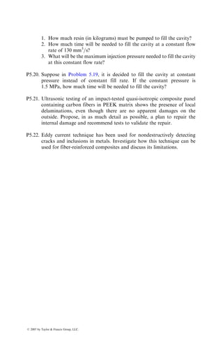
![The acoustic emission begins only after the applied load in the first cycle
exceeds a minimum value, and then the cumulative event count increases
rapidly with increasing load. If the specimen is unloaded, the acoustic emission
stops. If the load is reapplied, the acoustic emission occurs even before the
previous maximum load is reached. This unique AE characteristic of a fiber-
reinforced composite is not observed in metals and is called the felicity
effect [34]. The load at which the AE begins on the (n þ 1)th load cycle divided
by the maximum load reached on the nth load cycle is termed the felicity ratio.
The value of the felicity ratio indicates the extent of damage in the material and
can be used as a potential acceptance or rejection criterion [35].
The difference in arrival times of a given event at various transducers can be
used to locate the source of an acoustic emission. However, since a fiber-
reinforced composite structure emits numerous bursts of emission in successive
order, the transducers may not always be able to isolate a specific event.
Furthermore, signal attenuation in fiber-reinforced polymers is high. Since
low-frequency waves (typically 20–111 kHz) attenuate less and therefore travel
longer distances than high-frequency waves, transducers designed to detect this
frequency range are preferred for fiber-reinforced composite structures. Usu-
ally, high-frequency transducers are used in local areas of probable emission in
conjunction with low-frequency transducers.
Acoustic emission has been used by a number of investigators to study the
development and progression of damage with increasing time or stress. Some of
these studies have also included the effects of various process and material
parameters, such as cure temperature, cooling rate, matrix flexibility, and fiber
orientation, on the acoustic emission activities of fiber-reinforced polymers.
Standard practices have been developed for acoustic emission testing of glass
fiber-reinforced plastic tanks and pressure vessels [36]. However, as Hamstad
[37] has noted, acoustic emission in fiber-reinforced composites is a complex
phenomenon and may lead to erroneous source identification if proper
attention is not paid to the nature of wave attenuation and extraneous noise
generation.
5.9.3.4 Acousto-Ultrasonic
Acousto-ultrasonic testing combines aspects of ultrasonic testing with acoustic
emission signal analysis techniques to measure the severity of subtle internal
flaws and inhomogeneity in a material. Examples of such flaws in a composite
material are porosity, fiber breaks, fiber bunching, resin-rich zones, improper
curing, fiber misorientations, and fiber–matrix debonding. While these flaws are
not always considered as critical as delaminations or large voids, collectively they
can reduce the mechanical properties or structural response of a material [38].
In acousto-ultrasonic method, a broad-band piezoelectric transducer is
used to introduce a series of repeating ultrasonic pulses in the material. When
these pulses interact with various flaws in the material, spontaneous stress
ß 2007 by Taylor Francis Group, LLC.](https://image.slidesharecdn.com/fiberreinforcedcompositesmaterialsmanufacturinganddesignp1-220510152925-9ef3de0d/85/Fiber_Reinforced_Composites_Materials_Manufacturing_and_Design_P-1-pdf-468-320.jpg)
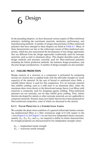
![subjected to a uniform heat source on one surface, the heat flow through its
thickness will be uneven as a result of local variation of thermal conductivity.
This will result in a nonuniform surface temperature distribution, which is
detected and related to the presence of defects in the interior of the material
[39]. For example, heat flow obstructed by a delaminated area increases the
surface temperature above the delaminated area compared with that in the
surrounding area (Figure 5.54).
The most common technique in thermography is to apply a uniform heat
source on one surface of the material and record the transient temperature
contours on the other surface by means of either liquid crystals or an infrared
heat detection camera. The heat source can be as simple as hot water bags, hot
air-dryers, a bank of light bulbs, or a photographic flash gun. Planar location
and planar size of the defect can be easily detected from the thermogram.
A modified form of thermography is called vibrothermography [40], in
which low-amplitude mechanical vibrations are used to induce localized heat-
ing in the material. It has been observed that localized heating occurs prefer-
entially around internal defects, such as delaminations and large matrix cracks.
The resulting temperature contours are recorded as before.
0
0
50
ΔT (⬚C)
T
(⬚C)
100
4
Time (seconds)
Heating Cooling
Away from
delamination
Delaminated
area
8 12
10
5
0
FIGURE 5.54 Surface temperature difference over delaminated and away from delami-
nated areas in a eight-ply carbon fiber–epoxy laminate. The delamination size is 5 mm
between plies 1 and 2. (Adapted from Mirchandani, M.G. and McLaughlin, P.V., Jr.,
Quantitative Nondestructive Evaluation, Vol. 5B, Plenum Press, New York, 1986.)
ß 2007 by Taylor Francis Group, LLC.](https://image.slidesharecdn.com/fiberreinforcedcompositesmaterialsmanufacturinganddesignp1-220510152925-9ef3de0d/85/Fiber_Reinforced_Composites_Materials_Manufacturing_and_Design_P-1-pdf-470-320.jpg)
![5.10 COST ISSUES
One major obstacle to greater use of fiber-reinforced composites in structural
applications is their cost. Although carbon fiber-reinforced composites are used
in large quantities in aerospace applications, their high cost is still a concern.
The automotive industry is significantly more cost-conscious and has used
carbon fiber-reinforced composites in a very limited amount. Most of the
structural composite parts used in automobiles today are manufactured from
glass fiber-reinforced polyesters or vinyl esters using compression molding
or glass fiber-reinforced polyurethane using SRIM. Even with their lower
cost, they cannot always compete with low carbon steel, which is less than
half as expensive. It has been shown that carbon fiber-reinforced polymers can
greatly reduce the weight of automotive body and chassis components due to
their high modulus–weight ratio and fatigue resistance, but the high cost of
carbon fibers has prevented their use in the automotive industry. The same
argument can be made for many other nonaerospace industries as well.
The high cost of fibers is not the only reason for the high cost of fiber-
reinforced polymers. The cost of the matrix can also be very high, especially if it
is a high-temperature polymer. For the total material cost, one must also
include the cost of preparing the material, for example, for making prepreg
or for making sheet-molding compound sheet. The standard unidirectional
carbon fiber–epoxy prepreg is typically about 1.5–2 times the cost of carbon
fibers [41]. The cost of making toughened epoxy prepreg or high temperature
thermoplastic matrix prepreg can be as much as three times higher than that of
making standard epoxy prepregs.
The second item in the cost consideration is the fabrication cost of fiber-
reinforced polymer parts, which depends on part design and the manufacturing
process selected for fabrication. In the early days of composite applications in the
aerospace industry, hand layup of prepreg stacks followedby vacuum bagging and
autoclave curing was the most common method of producing carbon fiber-
reinforced epoxy parts. The processing steps involved in autoclave molding are
1. Cutting the prepreg material (template layout, actual cutting and mark-
ing of the cut plies)
2. Laying up the plies (orienting the plies, building up the stack, and
tacking or debulking)
3. Bagging and autoclave preparation
4. Autoclave cycle
5. Demolding
6. Trimming the part to final dimensions
7. Inspection, including nondestructive testing
Most of the operations involved in autoclave molding are done manually,
may take several minutes to several hours, and require the use of highly
ß 2007 by Taylor Francis Group, LLC.](https://image.slidesharecdn.com/fiberreinforcedcompositesmaterialsmanufacturinganddesignp1-220510152925-9ef3de0d/85/Fiber_Reinforced_Composites_Materials_Manufacturing_and_Design_P-1-pdf-471-320.jpg)
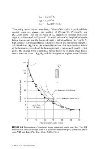
![technique for many of these defects is the through-transmission ultrasonic
testing. Depending on the part complexity and the level as well as frequency
of inspection needed, the cost of quality inspection can be in the range of 25%–
100% of the fabrication cost [41].
REFERENCES
1. W.I. Lee, A.C. Loos, and G.S. Springer, Heat of reaction, degree of cure, and
viscosity of Hercules 3501-6 resin, J. Compos. Mater., 16:510 (1982).
2. K.W. Lem and C.D. Han, Thermokinetics of unsaturated polyester and vinyl ester
resins, Polym. Eng. Sci., 24:175 (1984).
3. D.S. Lee and C.D. Han, Chemorheology and curing behavior of low-profile poly-
ester resin, Proceedings 40th Annual Technical Conference, Society of the Plastics
Industry, January (1985).
4. M.R. Kamal and S. Sourour, Kinetics and thermal characterization of thermoset
cure, Polym. Eng, Sci., 13:59 (1973).
5. M.R. Kamal, Thermoset characterization for moldability analysis, Polym. Eng. Sci.,
14:231 (1974).
6. B.R. Gebart, Permeability of unidirectional reinforcements in RTM, J. Compos.
Mater., 26:1100 (1992).
7. P. Hubert and A. Poursartip, A review of flow and compaction modelling relevant
to thermoset matrix laminate processing, J. Reinf. Plast. Compos., 17:286 (1998).
8. T.G. Gutowski, T. Morgaki, and Z. Cai, The consolidation of laminate composites,
J. Compos. Mater., 21:172 (1987).
9. A.C. Loos and G.S. Springer, Curing of epoxy matrix composites, J. Compos.
Mater., 17:135 (1983).
10. Structural Composites Fabrication Guide, Vol. 1, Manufacturing Technology Divi-
sion, U.S. Air Force Materials Laboratory (1982).
11. P.K. Mallick, Compression molding, Composite Materials Technology (P.K.
Mallick and S. Newman, eds.), Hanser Publishers, New York (1990).
12. L.F. Marker and B. Ford, Flow and curing behavior of SMC during molding, Mod.
Plast., 54:64 (1977).
13. P.J. Costigan, B.C. Fisher, and M. Kanagendra, The rheology of SMC during
compression molding and resultant material properties, Proceedings 40th Annual
Conference, Society of the Plastics Industry, January (1985).
14. M.R. Barone and D.A. Caulk, Kinematics of flow in sheet molding compounds,
Polym. Compos., 6:105 (1985).
15. R.M. Griffith and H. Shanoski, Reducing blistering in SMC molding, Plast. Des.
Process., 17:10 (1977).
16. P.K. Mallick, Effect of fiber misorientation on the tensile strength of compression
molded continuous fiber composites, Polym. Compos., 7:14 (1986).
17. R.B. Jutte, SMC-sink mechanisms and techniques of minimizing sing, International
Automotive Engineering Congress, Detroit, Paper No. 730171, Society of Automo-
tive Engineers (1973).
18. K.L. Smith and N.P. Suh, An approach towards the reduction of sink marks in
sheet molding compound, Polym. Eng. Sci., 19:829 (1979).
ß 2007 by Taylor Francis Group, LLC.](https://image.slidesharecdn.com/fiberreinforcedcompositesmaterialsmanufacturinganddesignp1-220510152925-9ef3de0d/85/Fiber_Reinforced_Composites_Materials_Manufacturing_and_Design_P-1-pdf-473-320.jpg)
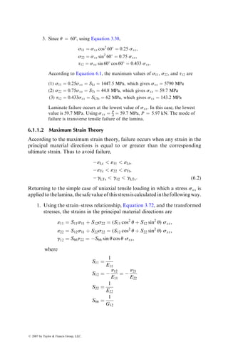
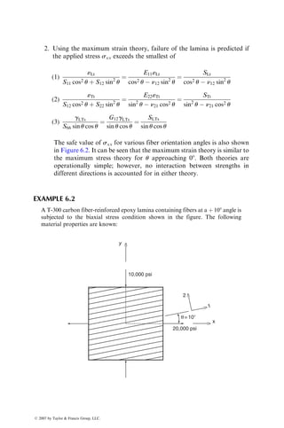
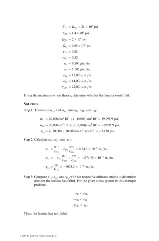
![P5.6. The following isothermal viscosity data were obtained in a parallel-plate
viscometer for an epoxy system cured at 1258C:
Time (min) Viscosity (cP)
0 79.5
20 100
40 148
60 162
80 263
100 512
120 1,480
140 6,160
160 44,600
180 513,000
200 14,781,000
Plot the data on a semilog scale and schematically show how the nature
of this curve may change if (a) the curing temperature is 1508C, (b) the
curing temperature is 1008C, and (c) the epoxy system is B-staged before
curing at 1258C.
P5.7. Lee et al. [1] fitted the following equation to the viscosity (h) data (in Pa s)
for an epoxy system:
h ¼ 7:9 1014
exp
E
RT
þ 14ac
for ac 0:5,
where
E ¼ activation energy for viscosity ¼ 9 3 104
J=mol
R ¼ universal gas constant (J=mol K)
T ¼ absolute temperature (K)
ac ¼ degree of cure
Using this equation, estimate the viscosity of the epoxy system at 1008C
and 1508C (a) at the beginning of the curing reaction, (b) at 20% cure,
and (c) at 40% cure.
P5.8. Roller* has represented the isothermal viscosity data for a B-staged
epoxy resin, by the following four-parameter equation:
* M.B. Roller, Characterization of the time–temperature–viscosity behavior of curing B-staged
epoxy resin, Polym. Eng. Sci., 15:406 (1975).
ß 2007 by Taylor Francis Group, LLC.](https://image.slidesharecdn.com/fiberreinforcedcompositesmaterialsmanufacturinganddesignp1-220510152925-9ef3de0d/85/Fiber_Reinforced_Composites_Materials_Manufacturing_and_Design_P-1-pdf-477-320.jpg)
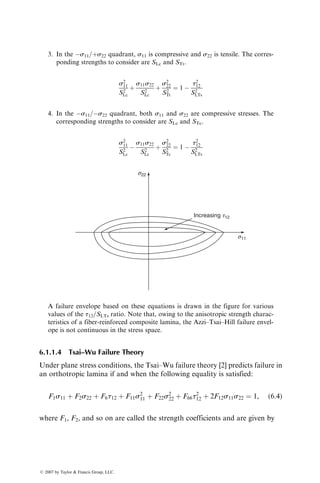
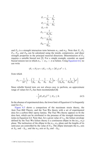
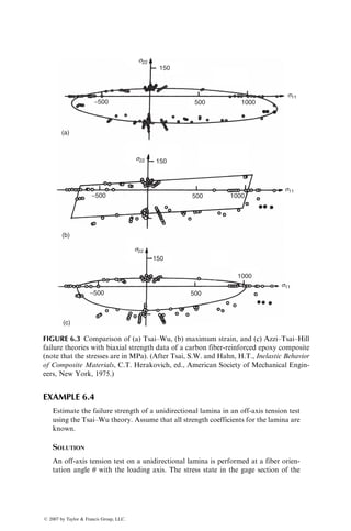
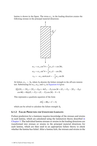
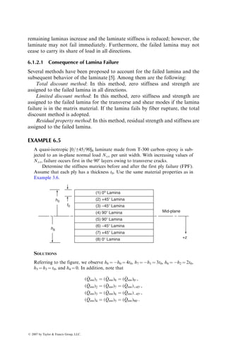
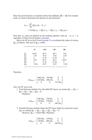
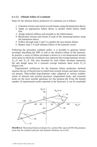
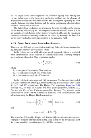
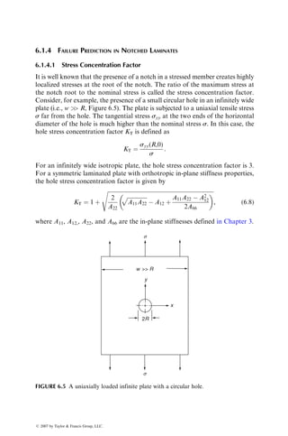
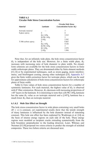
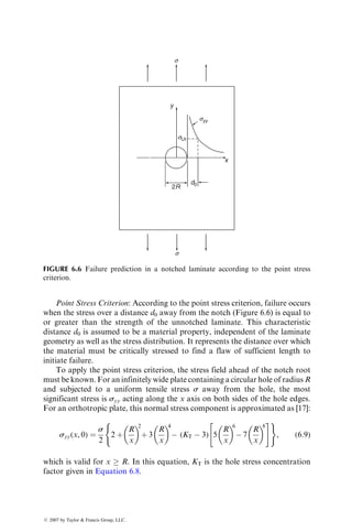
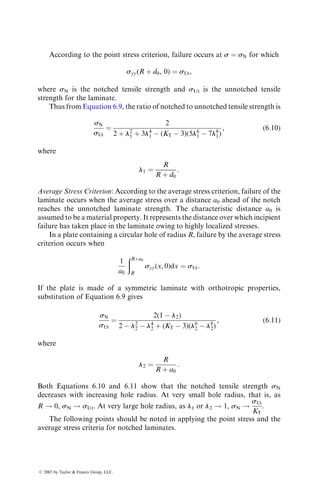
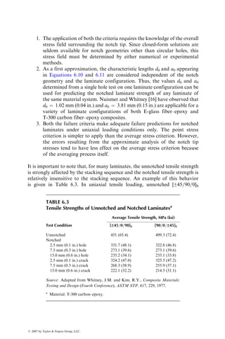
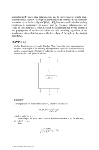
![6.1.1.3 Azzi–Tsai–Hill Theory
Following Hill’s anisotropic yield criterion for metals, Azzi and Tsai [1]
proposed that failure occurs in an orthotropic lamina if and when the following
equality is satisfied:
s2
11
S2
Lt
s11s22
S2
Lt
þ
s2
22
S2
Tt
þ
t2
12
S2
LTs
¼ 1, (6:3)
where s11 and s22 are both tensile (positive) stresses. When s11 and s22 are
compressive, the corresponding compressive strengths are used in Equation 6.3.
For the uniaxial tensile stress situation considered earlier, failure is
predicted if
sxx
1
cos4
u
S2
Lt
sin2
u cos2
u
S2
Lt
þ
sin4
u
S2
Tt
þ
sin2
u cos2
u
S2
Lts
1=2
:
This equation, plotted in Figure 6.2, indicates a better match with experimental
data than the maximum stress or the maximum strain theories.
EXAMPLE 6.3
Determine and draw the failure envelope for a general orthotropic lamina using
Azzi–Tsai–Hill theory.
SOLUTION
A failure envelope is a graphic representation of failure theory in the stress
coordinate system and forms a boundary between the safe and unsafe design
spaces. Selecting s11 and s22 as the coordinate axes and rearranging Equation
6.3, we can represent the Azzi–Tsai–Hill failure theory by the following equations.
1. In the þs11=þs22 quadrant, both s11 and s22 are tensile stresses. The corre-
sponding strengths to consider are SLt and STt.
s2
11
S2
Lt
s11s22
S2
Lt
þ
s2
22
S2
Tt
¼ 1
t2
12
S2
LTs
2. In the þs11=s22 quadrant, s11 is tensile and s22 is compressive. The corres-
ponding strengths to consider are SLt and STc.
s2
11
S2
Lt
þ
s11s22
S2
Lt
þ
s2
22
S2
Tc
¼ 1
t2
12
S2
LTs
ß 2007 by Taylor Francis Group, LLC.](https://image.slidesharecdn.com/fiberreinforcedcompositesmaterialsmanufacturinganddesignp1-220510152925-9ef3de0d/85/Fiber_Reinforced_Composites_Materials_Manufacturing_and_Design_P-1-pdf-492-320.jpg)
![3. In the s11=þs22 quadrant, s11 is compressive and s22 is tensile. The corres-
ponding strengths to consider are SLc and STt.
s2
11
S2
Lc
þ
s11s22
S2
Lc
þ
s2
22
S2
Tt
¼ 1
t2
12
S2
LTs
4. In the s11=s22 quadrant, both s11 and s22 are compressive stresses. The
corresponding strengths to consider are SLc and STc.
s2
11
S2
Lc
s11s22
S2
Lc
þ
s2
22
S2
Tc
¼ 1
t2
12
S2
LTs
s22
s11
Increasing t12
A failure envelope based on these equations is drawn in the figure for various
values of the t12=SLTs ratio. Note that, owing to the anisotropic strength charac-
teristics of a fiber-reinforced composite lamina, the Azzi–Tsai–Hill failure envel-
ope is not continuous in the stress space.
6.1.1.4 Tsai–Wu Failure Theory
Under plane stress conditions, the Tsai–Wu failure theory [2] predicts failure in
an orthotropic lamina if and when the following equality is satisfied:
F1s11 þ F2s22 þ F6t12 þ F11s2
11 þ F22s2
22 þ F66t2
12 þ 2F12s11s22 ¼ 1, (6:4)
where F1, F2, and so on are called the strength coefficients and are given by
ß 2007 by Taylor Francis Group, LLC.](https://image.slidesharecdn.com/fiberreinforcedcompositesmaterialsmanufacturinganddesignp1-220510152925-9ef3de0d/85/Fiber_Reinforced_Composites_Materials_Manufacturing_and_Design_P-1-pdf-493-320.jpg)
![F1 ¼
1
SLt
1
SLc
F2 ¼
1
STt
1
STc
F6 ¼ 0
F11 ¼
1
SLtSLc
F22 ¼
1
STtSTc
F66 ¼
1
S2
LTs
and F12 is a strength interaction term between s11 and s22. Note that F1, F2,
F11, F22, and F66 can be calculated using the tensile, compressive, and shear
strength properties in the principal material directions. Determination of F12
requires a suitable biaxial test [3]. For a simple example, consider an equal
biaxial tension test in which s11 ¼ s12 ¼ s at failure. Using Equation 6.4, we
can write
(F1 þ F2) s þ (F11 þ F22 þ 2F12) s2
¼ 1,
from which
F12 ¼
1
2s2
1
1
SLt
1
SLc
þ
1
STt
1
STc
s
1
SLtSLc
þ
1
STtSTc
s2
:
Since reliable biaxial tests are not always easy to perform, an approximate
range of values for F12 has been recommended [4]:
1
2
(F11F22)1=2
F12 0: (6:5)
In the absence of experimental data, the lower limit of Equation 6.5 is frequently
used for F12.
Figure 6.3 shows a comparison of the maximum strain theory, the
Azzi–Tsai–Hill Theory, and the Tsai–Wu theory with a set of experimental
data for a carbon fiber–epoxy lamina. The Tsai–Wu theory appears to fit the
data best, which can be attributed to the presence of the strength interaction
terms in Equation 6.4. Note that, for a given value of t12, the failure envelope
defined by the Tsai–Wu failure theory is a continuous ellipse in the (s11, s22)
plane. The inclination of the ellipse in the s11, s22 plane and the lengths of its
semi-axes are controlled by the value of F12. The ellipse intercepts the s11 axis
at SLt and SLc, and the s22 axis at STt and STc.
ß 2007 by Taylor Francis Group, LLC.](https://image.slidesharecdn.com/fiberreinforcedcompositesmaterialsmanufacturinganddesignp1-220510152925-9ef3de0d/85/Fiber_Reinforced_Composites_Materials_Manufacturing_and_Design_P-1-pdf-494-320.jpg)
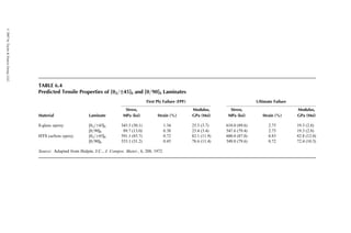
![lamina is shown in the figure. The stress sxx in the loading direction creates the
following stresses in the principal material directions:
q
s11 ¼ sxx cos2
u ¼
1
2
sxx(1 þ cos 2u),
s22 ¼ sxx sin2
u ¼
1
2
sxx(1 cos 2u),
t12 ¼ sxx sin u cos u ¼
1
2
sxx sin 2u:
At failure, sxx ¼ Su, where Su denotes the failure strength in the off-axis tension
test. Substituting for s11, s22, and t12 in Equation 6.4 gives
S2
u[(3F11 þ 3F22 þ 2F12 þ F66) þ 4(F11 F22) cos 2u þ (F11 þ F22 2F12 F66)
cos 4u] þ 4Su[(F1 þ F2) þ (F1 F2) cos 2u] 8 ¼ 0:
This represents a quadratic equation of the form
AS2
u þ BSu þ C ¼ 0,
which can be solved to calculate the failure strength Su.
6.1.2 FAILURE PREDICTION FOR UNNOTCHED LAMINATES
Failure prediction for a laminate requires knowledge of the stresses and strains
in each lamina, which are calculated using the lamination theory described in
Chapter 3. The individual lamina stresses or strains in the loading directions are
transformed into stresses or strains in the principal material directions for
each lamina, which are then used in an appropriate failure theory to check
whether the lamina has failed. After a lamina fails, the stresses and strains in the
ß 2007 by Taylor Francis Group, LLC.](https://image.slidesharecdn.com/fiberreinforcedcompositesmaterialsmanufacturinganddesignp1-220510152925-9ef3de0d/85/Fiber_Reinforced_Composites_Materials_Manufacturing_and_Design_P-1-pdf-496-320.jpg)
![remaining laminas increase and the laminate stiffness is reduced; however, the
laminate may not fail immediately. Furthermore, the failed lamina may not
cease to carry its share of load in all directions.
6.1.2.1 Consequence of Lamina Failure
Several methods have been proposed to account for the failed lamina and the
subsequent behavior of the laminate [5]. Among them are the following:
Total discount method: In this method, zero stiffness and strength are
assigned to the failed lamina in all directions.
Limited discount method: In this method, zero stiffness and strength are
assigned to the failed lamina for the transverse and shear modes if the lamina
failure is in the matrix material. If the lamina fails by fiber rupture, the total
discount method is adopted.
Residual property method: In this method, residual strength and stiffness are
assigned to the failed lamina.
EXAMPLE 6.5
A quasi-isotropic [0=±45=90]S laminate made from T-300 carbon–epoxy is sub-
jected to an in-plane normal load Nxx per unit width. With increasing values of
Nxx, failure occurs first in the 908 layers owing to transverse cracks.
Determine the stiffness matrices before and after the first ply failure (FPF).
Assume that each ply has a thickness t0. Use the same material properties as in
Example 3.6.
h0
(1) 0o
Lamina
(8) 0⬚ Lamina
(2) +45⬚ Lamina
(7) +45⬚ Lamina
(3) −45⬚ Lamina
(6) −45⬚ Lamina
(4) 90⬚ Lamina Mid-plane
+z
(5) 90⬚ Lamina
h8
t0
SOLUTIONS
Referring to the figure, we observe h8 ¼ h0 ¼ 4t0, h7 ¼ h1 ¼ 3t0, h6 ¼ h2 ¼ 2t0,
h5 ¼ h3 ¼ t0, and h4 ¼ 0. In addition, note that
(
Qmn)1 ¼ (
Qmn)8 ¼ (
Qmn)0 ,
(
Qmn)2 ¼ (
Qmn)7 ¼ (
Qmn)þ45 ,
(
Qmn)3 ¼ (
Qmn)6 ¼ (
Qmn)45 ,
(
Qmn)4 ¼ (
Qmn)5 ¼ (
Qmn)90 :
ß 2007 by Taylor Francis Group, LLC.](https://image.slidesharecdn.com/fiberreinforcedcompositesmaterialsmanufacturinganddesignp1-220510152925-9ef3de0d/85/Fiber_Reinforced_Composites_Materials_Manufacturing_and_Design_P-1-pdf-497-320.jpg)
![Since the given laminate is symmetric about the midplane, [B] ¼ [0]. For in-plane
loads, we need to determine the elements in the [A] matrix.
Amn ¼
X
8
j¼1
(
Qmn)j(hj hj1)
¼ 2t0[(
Qmn)0 þ (
Qmn)þ45 þ (
Qmn)45 þ (Qmn)90 ]:
Note that Amn does not depend on the stacking sequence, since (hj hj1) ¼ t0
regardless of where the jth lamina is located.
Before the 908 layers fail: From Example 3.6, we tabulate the values of various
Qmn as follows. The unit of
Qmn is GPa.
08 1458 458 908
Q11 134.03 40.11 40.11 8.82
Q12 2.29 33.61 33.61 2.29
Q16 0 31.30 31.30 0
Q22 8.82 40.11 40.11 134.03
Q26 0 31.30 31.30 0
Q66 3.254 34.57 34.57 3.254
Therefore,
[A]before ¼
446:14t0 143:60t0 0
143:60t0 446:14t0 0
0 0 151:30t0
2
4
3
5:
After the 908 layers fail:
1. Total discount method: For the failed 908 layers, we assume
Q11 ¼
Q12 ¼
Q16 ¼
Q22 ¼
Q26 ¼
Q66 ¼ 0.
Therefore,
[A]after ¼
428:50t0 139:02t0 0
139:02t0 178:08t0 0
0 0 144:79t0
2
4
3
5
2. Limited discount method: Since the 908 layers failed by transverse crack-
ing, we assume
Q11 ¼
Q12 ¼
Q16 ¼
Q26 ¼
Q66 ¼ 0:
However,
Q22 ¼ 134:03 GPa. Therefore,
[A]after ¼
428:50t0 139:02t0 0
139:02t0 446:14t0 0
0 0 144:79t0
2
4
3
5
ß 2007 by Taylor Francis Group, LLC.](https://image.slidesharecdn.com/fiberreinforcedcompositesmaterialsmanufacturinganddesignp1-220510152925-9ef3de0d/85/Fiber_Reinforced_Composites_Materials_Manufacturing_and_Design_P-1-pdf-498-320.jpg)
![6.1.2.2 Ultimate Failure of a Laminate
Steps for the ultimate failure prediction of a laminate are as follows.
1. Calculate stresses and strains in each lamina using the lamination theory
2. Apply an appropriate failure theory to predict which lamina failed
first
3. Assign reduced stiffness and strength to the failed lamina
4. Recalculate stresses and strains in each of the remaining laminas using
the lamination theory
5. Follow through steps 2 and 3 to predict the next lamina failure
6. Repeat steps 2–4 until ultimate failure of the laminate occurs
Following the procedure outlined earlier, it is possible to generate failure
envelopes describing the FPF as well as the ultimate failure of the laminate.
In practice, a series of failure envelopes is drawn in a two-dimensional normal
stress space in which the coordinate axes represent the average laminate stresses
Nxx=h and Nyy=h. The area bounded by each failure envelope represents
the safe design space for a constant average laminate shear stress Nxy=h
(Figure 6.4).
Experimental verification for the laminate failure prediction methods
requires the use of biaxial tests in which both normal stresses and shear stresses
are present. Thin-walled large-diameter tubes subjected to various combin-
ations of internal and external pressures, longitudinal loads, and torsional
loads are the most suitable specimens for this purpose [6]. From the limited
number of experimental results reported in the literature, it can be concluded
Nyy /h
Nxx /h
Nxy /h=0
−100 −75 75
10
10
100
20
20
50
50
−50
−50
25
25
−25
−25
FIGURE 6.4 Theoretical failure envelopes for a carbon fiber–epoxy [0=90±45]S laminate
(note that the in-plane loads per unit laminate thickness are in ksi).
ß 2007 by Taylor Francis Group, LLC.](https://image.slidesharecdn.com/fiberreinforcedcompositesmaterialsmanufacturinganddesignp1-220510152925-9ef3de0d/85/Fiber_Reinforced_Composites_Materials_Manufacturing_and_Design_P-1-pdf-499-320.jpg)
![that no single failure theory represents all laminates equally well. Among the
various deficiencies in the theoretical prediction methods are the absence of
interlaminar stresses and nonlinear effects. The assumption regarding the load
transfer between the failed laminas and the active laminas can also introduce
errors in the theoretical analyses.
The failure load prediction for a laminate depends strongly on the lamina
failure theory selected [7]. In the composite material industry, there is little
agreement on which lamina failure theory works best, although the maximum
strain theory is more commonly used than the others [8]. Recently, the Tsai–Wu
failure theory is finding more applications in the academic field.
6.1.3 FAILURE PREDICTION IN RANDOM FIBER LAMINATES
There are two different approaches for predicting failure in laminates contain-
ing randomly oriented discontinuous fibers.
In the Hahn’s approach [9], which is a simple approach, failure is predicted
when the maximum tensile stress in the laminate equals the following strength
averaged over all possible fiber orientation angles:
Sr ¼
4
p
ffiffiffiffiffiffiffiffiffiffiffiffiffi
SLtSTt
p
, (6:6)
where
Sr ¼ strength of the random fiber laminate
SLt ¼ longitudinal strength of a 08 laminate
STt ¼ transverse strength of a 08 laminate
In the Halpin–Kardos approach [10], the random fiber laminate is modeled
as a quasi-isotropic [0=±45=90]S laminate containing discontinuous fibers in the
08, ±458, and 908 orientations. The Halpin–Tsai equations, Equations 3.49
through 3.53, are used to calculate the basic elastic properties, namely, E11,
E22, n12, and G12, of the 08 discontinuous fiber laminas. The ultimate strain
allowables for the 08 and 908 laminas are estimated from the continuous fiber
allowables using the Halpin–Kardos equations:
«Lt(d) ¼ «Lt
Ef
Em
0:87
þ 0:50
#
for lf lc (6:7)
and
«Td(d) ¼ «Tt 1 1:21v
2=3
f
:
The procedure followed by Halpin and Kardos [10] for estimating the ultimate
strength of random fiber laminates is the same as the ply-by-ply analysis used
for continuous fiber quasi-isotropic [0=±45=90]S laminates.
ß 2007 by Taylor Francis Group, LLC.](https://image.slidesharecdn.com/fiberreinforcedcompositesmaterialsmanufacturinganddesignp1-220510152925-9ef3de0d/85/Fiber_Reinforced_Composites_Materials_Manufacturing_and_Design_P-1-pdf-500-320.jpg)
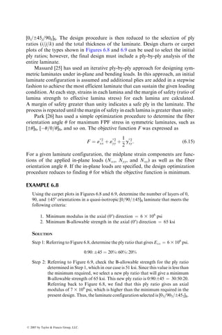
![Note that, for an infinitely wide plate, the hole stress concentration factor
KT is independent of the hole size. However, for a finite width plate, KT
increases with increasing ratio of hole diameter to plate width. No closed-
form solutions are available for the hole stress concentration factors in finite
width orthotropic plates. They are determined either by finite element methods
[11,12] or by experimental techniques, such as strain gaging, moire interfero-
metry, and birefringent coating, among other techniques [13]. Appendix A.7
gives the finite width correction factor for isotropic plates, which can be used
for approximate calculation of hole stress concentration factors for orthotropic
plates of finite width.
Table 6.2 lists values of hole stress concentration factors for a number of
symmetric laminates. For each material, the highest value of KT is observed
with 08 fiber orientation. However, KT decreases with increasing proportions of
±458 layers in the laminate. It is interesting to note that a [0=90=±45]S laminate
has the same KT value as an isotropic material and a [±458]S laminate has a
much lower KT than an isotropic material.
6.1.4.2 Hole Size Effect on Strength
The hole stress concentration factor in wide plates containing very small holes
(R w) is constant, yet experimental results show that the tensile strength
of many laminates is influenced by the hole diameter instead of remaining
constant. This hole size effect has been explained by Waddoups et al. [14] on
the basis of intense energy regions on each side of the hole. These energy
regions were modeled as incipient cracks extending symmetrically from the
hole boundary perpendicular to the loading direction. Later, Whitney and
Nuismer [15,16] proposed two stress criteria to predict the strength of notched
composites. These two failure criteria are discussed next.
TABLE 6.2
Circular Hole Stress Concentration Factors
Material Laminate
Circular Hole Stress
Concentration Factor (KT)
Isotropic material — 3
S-glass–epoxy 0 4
[02=±45]S 3.313
[0=90=±45]S 3
[±45]S 2.382
T-300 carbon–epoxy 0 6.863
[04=±45]S 4.126
[0=90=±45]S 3
[0=±45]S 2.979
[±45]S 1.984
ß 2007 by Taylor Francis Group, LLC.](https://image.slidesharecdn.com/fiberreinforcedcompositesmaterialsmanufacturinganddesignp1-220510152925-9ef3de0d/85/Fiber_Reinforced_Composites_Materials_Manufacturing_and_Design_P-1-pdf-502-320.jpg)
![Point Stress Criterion: According to the point stress criterion, failure occurs
when the stress over a distance d0 away from the notch (Figure 6.6) is equal to
or greater than the strength of the unnotched laminate. This characteristic
distance d0 is assumed to be a material property, independent of the laminate
geometry as well as the stress distribution. It represents the distance over which
the material must be critically stressed to find a flaw of sufficient length to
initiate failure.
To apply the point stress criterion, the stress field ahead of the notch root
must be known. For an infinitely wide plate containing a circular hole of radius R
and subjected to a uniform tensile stress s away from the hole, the most
significant stress is syy acting along the x axis on both sides of the hole edges.
For an orthotropic plate, this normal stress component is approximated as [17]:
syy(x, 0) ¼
s
2
2 þ
R
x
2
þ 3
R
x
4
(KT 3) 5
R
x
6
7
R
x
8
#
( )
, (6:9)
which is valid for x R. In this equation, KT is the hole stress concentration
factor given in Equation 6.8.
2R
d0
x
y
sUt
syy
s
s
FIGURE 6.6 Failure prediction in a notched laminate according to the point stress
criterion.
ß 2007 by Taylor Francis Group, LLC.](https://image.slidesharecdn.com/fiberreinforcedcompositesmaterialsmanufacturinganddesignp1-220510152925-9ef3de0d/85/Fiber_Reinforced_Composites_Materials_Manufacturing_and_Design_P-1-pdf-503-320.jpg)
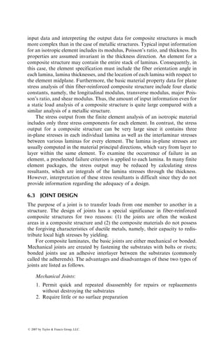
![1. The application of both the criteria requires the knowledge of the overall
stress field surrounding the notch tip. Since closed-form solutions are
seldom available for notch geometries other than circular holes, this
stress field must be determined by either numerical or experimental
methods.
2. As a first approximation, the characteristic lengths d0 and a0 appearing
in Equations 6.10 and 6.11 are considered independent of the notch
geometry and the laminate configuration. Thus, the values d0 and a0
determined from a single hole test on one laminate configuration can be
used for predicting the notched laminate strength of any laminate of
the same material system. Nuismer and Whitney [16] have observed that
d0 ¼ 1.02 mm (0.04 in.) and a0 ¼ 3.81 mm (0.15 in.) are applicable for a
variety of laminate configurations of both E-glass fiber–epoxy and
T-300 carbon fiber–epoxy composites.
3. Both the failure criteria make adequate failure predictions for notched
laminates under uniaxial loading conditions only. The point stress
criterion is simpler to apply than the average stress criterion. However,
the errors resulting from the approximate analysis of the notch tip
stresses tend to have less effect on the average stress criterion because
of the averaging process itself.
It is important to note that, for many laminates, the unnotched tensile strength
is strongly affected by the stacking sequence and the notched tensile strength is
relatively insensitive to the stacking sequence. An example of this behavior
is given in Table 6.3. In uniaxial tensile loading, unnotched [±45=90=0]S
TABLE 6.3
Tensile Strengths of Unnotched and Notched Laminatesa
Average Tensile Strength, MPa (ksi)
Test Condition [±45=0=90]S [90=0=±45]S
Unnotched 451 (65.4) 499.3 (72.4)
Notched
2.5 mm (0.1 in.) hole 331.7 (48.1) 322.8 (46.8)
7.5 mm (0.3 in.) hole 273.1 (39.6) 273.1 (39.6)
15.0 mm (0.6 in.) hole 235.2 (34.1) 233.1 (33.8)
2.5 mm (0.1 in.) crack 324.2 (47.0) 325.5 (47.2)
7.5 mm (0.3 in.) crack 268.3 (38.9) 255.9 (37.1)
15.0 mm (0.6 in.) crack 222.1 (32.2) 214.5 (31.1)
Source: Adapted from Whitney, J.M. and Kim, R.Y., Composite Materials:
Testing and Design (Fourth Conference), ASTM STP, 617, 229, 1977.
a
Material: T-300 carbon–epoxy.
ß 2007 by Taylor Francis Group, LLC.](https://image.slidesharecdn.com/fiberreinforcedcompositesmaterialsmanufacturinganddesignp1-220510152925-9ef3de0d/85/Fiber_Reinforced_Composites_Materials_Manufacturing_and_Design_P-1-pdf-505-320.jpg)
![laminates fail by gross edge delaminations due to the presence of tensile inter-
laminar normal stress szz throughout the thickness. In contrast, the interlaminar
normal stress at the free edges of [90=0=±45]S laminates under similar loading
conditions is compressive in nature and no free-edge delaminations are
found in these laminates. When notched, both laminates fail by the initiation
and propagation of tensile cracks from the hole boundary, regardless of the
interlaminar stress distributions at the free edges of the hole or the straight
boundaries.
EXAMPLE 6.6
Failure Prediction in a Centrally Cracked Plate. Using the point stress criterion,
estimate the strength of an infinitely wide symmetric laminated plate containing a
central straight crack of length 2c subjected to a uniform tensile stress applied
normal to the crack plane at infinity.
s
y
x
2c
s
SOLUTION
The expression for the normal stress syy ahead of the crack is
syy(x, 0) ¼
x
ffiffiffiffiffiffiffiffiffiffiffiffiffiffiffi
x2 c2
p s,
which is valid for x c.
According to the point stress criterion, failure occurs at s ¼ sN for which syy
(c þ d0, 0) ¼ sUt.
Thus,
(c þ d0)sN
ffiffiffiffiffiffiffiffiffiffiffiffiffiffiffiffiffiffiffiffiffiffiffiffiffiffiffiffi
(c þ d0)2
c2
p ¼ sUt
ß 2007 by Taylor Francis Group, LLC.](https://image.slidesharecdn.com/fiberreinforcedcompositesmaterialsmanufacturinganddesignp1-220510152925-9ef3de0d/85/Fiber_Reinforced_Composites_Materials_Manufacturing_and_Design_P-1-pdf-506-320.jpg)
![or
sN ¼ sUt
ffiffiffiffiffiffiffiffiffiffiffiffiffi
1 l2
3
q
,
where
l3 ¼
c
c þ d0
:
The mode I stress intensity factor for this condition can be written as
K1 ¼ sN
ffiffiffiffiffiffi
pc
p
¼ sUt
ffiffiffiffiffiffiffiffiffiffiffiffiffiffiffiffiffiffiffiffiffiffi
pc(1 l2
3)
q
:
6.1.5 FAILURE PREDICTION FOR DELAMINATION INITIATION
Delamination or ply separation due to interlaminar stresses is a critical failure
mode in many composite laminates. It can reduce the failure strength of some
laminates well below that predicted by the in-plane failure theories discussed in
Section 6.1.1.
Brewer and Lagace [18] as well as Zhou and Sun [19] proposed the following
quadratic failure criterion to predict the initiation of delamination at the free
edges:
s2
zz
S2
zt
þ
t2
xz
S2
xz
þ
t2
yz
S2
yz
¼ 1, (6:12)
where
Szt ¼ tensile strength in the thickness direction
Sxz, Syz ¼ interlaminar shear strengths
szz,
txz, and
tyz are the average interlaminar stresses defined by
(
szz,
txz,
tyz) ¼
1
xc
ðxc
0
(szz, txz, tyz)dx,
where xc is the critical distance over which the interlaminar stresses are
averaged.
Since the interlaminar strength data are not usually available, Zhou and
Sun [19] have suggested using Sxz ¼ Syz ¼ SLTs and Szt ¼ STt.. They also
recommend using xc equal to twice the ply thickness.
EXAMPLE 6.7
The average interlaminar shear stresses in a [±45]2S laminate under an in-plane
tensile force Nxx ¼ 410 kN=m are given as:
ß 2007 by Taylor Francis Group, LLC.](https://image.slidesharecdn.com/fiberreinforcedcompositesmaterialsmanufacturinganddesignp1-220510152925-9ef3de0d/85/Fiber_Reinforced_Composites_Materials_Manufacturing_and_Design_P-1-pdf-507-320.jpg)
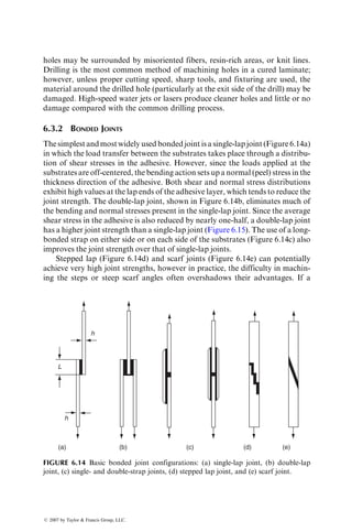
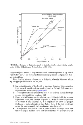
![TABLE 6.4
Predicted Tensile Properties of [02=±45]S and [0=90]S Laminates
First Ply Failure (FPF) Ultimate Failure
Material Laminate
Stress,
MPa (ksi) Strain (%)
Modulus,
GPa (Msi)
Stress,
MPa (ksi) Strain (%)
Modulus,
GPa (Msi)
S-glass–epoxy [02=±45]S 345.5 (50.1) 1.34 25.5 (3.7) 618.0 (89.6) 2.75 19.3 (2.8)
[0=90]S 89.7 (13.0) 0.38 23.4 (3.4) 547.6 (79.4) 2.75 19.3 (2.8)
HTS carbon–epoxy [02=±45]S 591.1 (85.7) 0.72 82.1 (11.9) 600.0 (87.0) 0.83 82.8 (12.0)
[0=90]S 353.1 (51.2) 0.45 78.6 (11.4) 549.0 (79.6) 0.72 72.4 (10.5)
Source: Adapted from Halpin, J.C., J. Compos. Mater., 6, 208, 1972.
ß
2007
by
Taylor
Francis
Group,
LLC.](https://image.slidesharecdn.com/fiberreinforcedcompositesmaterialsmanufacturinganddesignp1-220510152925-9ef3de0d/85/Fiber_Reinforced_Composites_Materials_Manufacturing_and_Design_P-1-pdf-510-320.jpg)
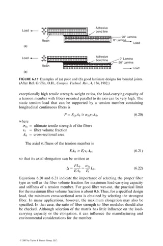
![the lamination theory along with a ply-level material property database.
Considering the wide variety of lamination possibilities with a given fiber–
resin combination, the second method is preferred by many designers since it
has the flexibility of creating new design allowables without recourse to extensive
testing.
The ply-level database is generated by testing unnotched unidirectional
specimens in the tension, compression, and shear modes. The basic character-
istics of the lamina, such as its longitudinal, transverse, and shear moduli,
Poisson’s ratios, and longitudinal, transverse, and shear strengths, as well as
strains-to-failure, are determined by the various static test procedures described
in Chapter 4. These tests are usually performed at room temperature; however,
the actual application environment should also be included in the test program.
The lamination theory combined with a failure criterion and a definition of
failure is then used to predict the design allowables for the selected lamination
configuration. This approach is particularly advantageous in generating design
charts (also called carpet plots) for a family of laminates with the same basic ply
orientations. Two of these charts for the [0=±45=90]S family of a carbon fiber–
epoxy composite are shown in Figures 6.8 and 6.9. Such charts are very useful
in selecting the proportions of the various ply orientations required to meet the
particular design criteria involved [20].
Owing to the statistical nature of the ultimate properties, the design
allowable strengths and strains are usually presented on one of the follow-
ing bases:
y
x
100
80
60
50
40
30
20
10
70
90
0
0
69
138
207
0
0
10
20
30
20 40 60 80 100
Percent ±458 plies
Percent 0⬚ plies
08
Tensile
modulus,
E
xx
(Msi)
E
xx
(GPa)
FIGURE 6.8 Carpet plot for tensile modulus Exx of a carbon fiber–epoxy [0=90=±45]S
laminate family. Note that the percentage of 908 plies is equal to 100 (percentage of 08
plies) (percentage of ±458 plies).
ß 2007 by Taylor Francis Group, LLC.](https://image.slidesharecdn.com/fiberreinforcedcompositesmaterialsmanufacturinganddesignp1-220510152925-9ef3de0d/85/Fiber_Reinforced_Composites_Materials_Manufacturing_and_Design_P-1-pdf-512-320.jpg)
![1. A basis: Designed on the A-basis strength or strain, a component has at
least a 99% probability of survival with a confidence level of 95%.
2. B basis: Designed on the B-basis strength or strain, a component has at
least a 90% probability of survival with a confidence level of 95%.
Statistical methods to generate A- and B-basis design allowables are briefly
described in Appendix A.8. The B-basis design allowables are commonly used
for fiber-reinforced composite laminates, since the failure of one or more plies
in these materials does not always result in the loss of structural integrity.
Ekvall and Griffin [21] have described a step-by-step procedure of formulating
the B-basis design allowables for T-300 carbon fiber–epoxy unidirectional and
multidirectional laminates. Their approach also takes into account the effects
of a 4.76 mm (0.1875 in.) diameter hole on the design allowable static strengths
of these laminates.
In establishing the fatigue strength allowables for composite helicopter
structures, Rich and Maass [22] used the mean fatigue strength minus 3 stand-
ard deviations. They observed that extrapolating the tension–tension fatigue
data to the tension–compression or compression–compression mode may not
be applicable for composite materials since significant fatigue strength reduc-
tions are possible in these two modes. Ply-level static and fatigue tests in their
program were conducted under a room-temperature dry (RTD) as well as at an
elevated-temperature wet (ETW) condition. The ETW condition selected was
more severe than the actual design environment for helicopters. However, this
y
1035
690
345
0
0
100
80
60
40
20
0
0
50
100
150
Allowable
tensile
strength
(ksi)
Percent ±458 plies
(MPa)
x
08
100
90
80
70
60
50
40
30
20
10
Percent
08 plies
FIGURE 6.9 Carpet plot for tensile strength sxx of a carbon fiber–epoxy [0=90=±45]S
laminate family.
ß 2007 by Taylor Francis Group, LLC.](https://image.slidesharecdn.com/fiberreinforcedcompositesmaterialsmanufacturinganddesignp1-220510152925-9ef3de0d/85/Fiber_Reinforced_Composites_Materials_Manufacturing_and_Design_P-1-pdf-513-320.jpg)
![procedure of testing at an ETW exceeding the design condition allows the
designer to determine the allowable values for a variety of environmental
conditions within the range investigated by interpolation rather than by
extrapolation (Figure 6.10).
6.2.4 GENERAL DESIGN GUIDELINES
The principal steps in designing a composite laminate are
1. Selection of fiber, resin, and fiber volume fraction
2. Selection of the optimum fiber orientation in each ply and the lamina
stacking sequence
3. Selection of the number of plies needed in each orientation, which also
determines the final thickness of the part
Considering these variables, it is obvious that a large variety of laminates may
be created even if the ply orientations are restricted to a single family, such as a
[0=±45=90]S family. Thus in most cases there is no straightforward method of
designing a composite laminate unless the problem involves a simple structure,
such as a rod or a column, and the loading is uniaxial.
From the standpoint of design as well as analytic simplicity, symmetric
laminates are commonly preferred over unsymmetric laminates. This eliminates
the extension–bending coupling represented by the [B] matrix. The presence of
Dry
Design
condition
Wet
Elevated
Test temperature
Room
A
or
B
allowable
strength
Interpolated line
FIGURE 6.10 Linear interpolation method for determining design allowables.
ß 2007 by Taylor Francis Group, LLC.](https://image.slidesharecdn.com/fiberreinforcedcompositesmaterialsmanufacturinganddesignp1-220510152925-9ef3de0d/85/Fiber_Reinforced_Composites_Materials_Manufacturing_and_Design_P-1-pdf-514-320.jpg)
![extension–bending coupling is also undesirable from the stiffness standpoint,
since it reduces the effective stiffness of the laminate and thereby increases its
deflection, reduces the critical buckling loads, and decreases the natural fre-
quency of vibration. Similar but lesser effects are observed if the laminate has
bending–twisting coupling due to the presence of D16 and D26 terms. However,
unless the fibers are at 0, 90, or 0=90 combinations, a symmetric laminate
cannot be designed with D16 ¼ D26 ¼ 0.
The deleterious free-edge effects in a laminate can be reduced through
proper selection of lamina stacking sequence. If angle-ply laminates are used,
the layers with þu and u orientations should be alternated instead of in a
clustered configuration [23]. Thus, for example, an eight-layer laminate with
four layers of þu orientations and four layers of u orientations should be
designed as [þu=u=þu=u]S instead of [u=u=u=u]S or [u=u=þu=þu]S.
However, if a laminate contains 0, 90, and ±u layers, adjacent þu and u layers
shouldbeavoided.Forexample,inthequasi-isotropiclaminatefamilycontaining
0, 90, and ±45 layers, a [45=0=90=45]S configuration is preferred over a
[90=þ45=45=0]S or a [0=þ45=45=90]S configuration.
6.2.4.1 Laminate Design for Strength
When the state of stress in a structure is known and does not change during the
course of its service operation, the lamina orientations may be selected in the
following way [24].
Using the standard Mohr’s circle technique, determine the principal normal
loads and the principal directions. Analytically, the principal normal loads are
N1 ¼
1
2
(Nxx þ Nyy) þ
Nxx Nyy
2
2
þ N2
xy
#1=2
,
N2 ¼
1
2
(Nxx þ Nyy)
Nxx Nyy
2
2
þ N2
xy
#1=2
, (6:13)
and the principal direction with respect to the x axis is
tan 2u ¼
2Nxy
Nxx Nyy
: (6:14)
Select a [0i=90j]S cross-ply configuration with the 08 layers aligned in the
direction of the maximum principal load N1 and the 908 layers aligned in
the direction of the minimum principal load N2. Thus with respect to the x
axis, the laminate configuration is [ui=(90 þ u)j]S. The ratio of 08 to 908 plies, i=j,
is equal to the principal load ratio N1=N2.
When the stress state in a structure varies in direction or is unknown, a
common approach in laminate design is to make it quasi-isotropic, for example,
ß 2007 by Taylor Francis Group, LLC.](https://image.slidesharecdn.com/fiberreinforcedcompositesmaterialsmanufacturinganddesignp1-220510152925-9ef3de0d/85/Fiber_Reinforced_Composites_Materials_Manufacturing_and_Design_P-1-pdf-515-320.jpg)
![[0i=±45j=90k]S. The design procedure is then reduced to the selection of ply
ratios (i=j=k) and the total thickness of the laminate. Design charts or carpet
plots of the types shown in Figures 6.8 and 6.9 can be used to select the initial
ply ratios; however, the final design must include a ply-by-ply analysis of the
entire laminate.
Massard [25] has used an iterative ply-by-ply approach for designing sym-
metric laminates under in-plane and bending loads. In this approach, an initial
laminate configuration is assumed and additional plies are added in a stepwise
fashion to achieve the most efficient laminate that can sustain the given loading
condition. At each step, strains in each lamina and the margin of safety (ratio of
lamina strength to effective lamina stress) for each lamina are calculated.
A margin of safety greater than unity indicates a safe ply in the laminate. The
process is repeated until the margin of safety in each lamina is greater than unity.
Park [26] has used a simple optimization procedure to determine the fiber
orientation angle u for maximum FPF stress in symmetric laminates, such as
[±u]S, [u=0=u]S, and so on. The objective function F was expressed as
F ¼ «
2
xx þ «
2
yy þ
1
2
g
2
xy: (6:15)
For a given laminate configuration, the midplane strain components are func-
tions of the applied in-plane loads (Nxx, Nyy, and Nxy) as well as the fiber
orientation angle u. If the in-plane loads are specified, the design optimization
procedure reduces to finding u for which the objective function is minimum.
EXAMPLE 6.8
Using the carpet plots in Figures 6.8 and 6.9, determine the number of layers of 0,
90, and ±458 orientations in a quasi-isotropic [0=90=±45]S laminate that meets the
following criteria:
1. Minimum modulus in the axial (08) direction ¼ 6 3 106
psi
2. Minimum B-allowable strength in the axial (08) direction ¼ 65 ksi
SOLUTION
Step 1: Referring to Figure 6.8, determine the ply ratio that gives Exx ¼ 6 3 106
psi.
0:90: 45 ¼ 20%: 60%: 20%
Step 2: Referring to Figure 6.9, check the B-allowable strength for the ply ratio
determined in Step 1, which in our case is 51 ksi. Since this value is less than
the minimum required, we select a new ply ratio that will give a minimum
B-allowable strength of 65 ksi. This new ply ratio is 0:90:±45 ¼ 30:50:20.
Referring back to Figure 6.8, we find that this ply ratio gives an axial
modulus of 7 3 106
psi, which is higher than the minimum required in the
present design. Thus, the laminate configuration selected is [03=905=±452]S.
ß 2007 by Taylor Francis Group, LLC.](https://image.slidesharecdn.com/fiberreinforcedcompositesmaterialsmanufacturinganddesignp1-220510152925-9ef3de0d/85/Fiber_Reinforced_Composites_Materials_Manufacturing_and_Design_P-1-pdf-516-320.jpg)
![Step 3: Assuming that the ply thickness is 0.005 in., we determine the ply thickness
for each fiber orientation as
0
: 6 0:005 in: ¼ 0:03 in:
90
: 10 0:005 in: ¼ 0:05 in:
þ45
: 4 0:005 in: ¼ 0:02 in:
45
: 4 0:005 in: ¼ 0:02 in:
Thus, the total laminate thickness is 0.12 in.
6.2.4.2 Laminate Design for Stiffness
The stiffness of a member is a measure of its resistance to deformation or
deflection owing to applied loads. If the member is made of an isotropic
material, its stiffnesses are given by
Axial stiffness ¼ EA0,
Bending stiffness ¼ EIc,
Torsional stiffness ¼ GJc, (6:16)
where
E ¼ modulus of elasticity
G ¼ shear modulus
A0 ¼ cross-sectional area
Ic ¼ moment of inertia of the cross section about the neutral axis
Jc ¼ polar moment of inertia of the cross section
The stiffness equations for composite members are in general more involved
than those given in Equation 6.16. If the composite member is made of a
symmetric laminate, its stiffness against the in-plane loads is related to the
elements in the [A] matrix, whereas its stiffness against bending, buckling, and
torsional loads is related to the elements in the [D] matrix. The elements in both
[A] and [D] matrices are functions of the fiber type, fiber volume fraction, fiber
orientation angles, lamina thicknesses, and the number of layers of each orien-
tation. In addition, the elements in the [D] matrix depend strongly on the
lamina stacking sequence.
Except for 0, 90, and 0=90 combinations, the [D] matrix for all symmetric
laminates contains nonzero D16 and D26 terms. Closed-form solutions for
bending deflections, buckling loads, and vibrational frequencies of general
symmetric laminates are not available. The following closed-form solutions
[27,28] are valid for the special class of laminates for which D16 ¼ D26 ¼ 0
and the elements in the [B] matrix are negligible:
ß 2007 by Taylor Francis Group, LLC.](https://image.slidesharecdn.com/fiberreinforcedcompositesmaterialsmanufacturinganddesignp1-220510152925-9ef3de0d/85/Fiber_Reinforced_Composites_Materials_Manufacturing_and_Design_P-1-pdf-517-320.jpg)
![1. Center deflection of a simply supported rectangular plate carrying a
uniformly distributed load p0:
w ffi
16p0R4
b4
p6
1
D11 þ 2(D12 þ 2D66)R2 þ D22R4
(6:17)
2. Critical buckling load for a rectangular plate with pinned edges at the
ends of its long dimension:
Ncr ffi
p2
[D11 þ 2(D12 þ 2D66)R2
þ D22R4
]
b2R2
(6:18)
3. Fundamental frequency of vibration for a simply supported rectangular
plate:
f 2
ffi
p4
rR4b4
[D11 þ 2(D12 þ 2D66)R2
þ D22R4
] (6:19)
where
a ¼ plate length
b ¼ plate width
R ¼ plate aspect ratio ¼ a=b
r ¼ density of the plate material
A few closed-form solutions are also available in the literature for unsym-
metric laminates with a nonzero [B] matrix [27,28]. However, it has been shown
that the coupling effect of the [B] matrix becomes small when the laminate
contains more than six to eight layers [29]. Therefore, for most practical lamin-
ates, Equations 6.17 through 6.19 can be used for initial design purposes.
6.2.5 FINITE ELEMENT ANALYSIS
Design analysis of a laminated composite structure almost invariably requires
the use of computers to calculate stresses and strains in each ply and to inves-
tigate whether the structure is ‘‘safe.’’ For simple structures, such as a plate or a
beam, the design analysis can be performed relatively easily. If the structure and
the loading are complex, it may be necessary to perform the design analysis
using finite element analysis. Commercially available finite element softwares,
such as MSC-NASTRAN, ANSYS, ABAQUS, and LS-DYNA, have the cap-
ability of combining the lamination theory with the finite element codes. Many
of these packages are capable of calculating in-plane as well as interlaminar
stresses, incorporate more than one failure criterion, and contain a library of
plate, shell, or solid elements with orthotropic material properties [30].
Although finite element analyses for both isotropic materials and laminated
composite materials follow the same procedure, the problem of preparing the
ß 2007 by Taylor Francis Group, LLC.](https://image.slidesharecdn.com/fiberreinforcedcompositesmaterialsmanufacturinganddesignp1-220510152925-9ef3de0d/85/Fiber_Reinforced_Composites_Materials_Manufacturing_and_Design_P-1-pdf-518-320.jpg)
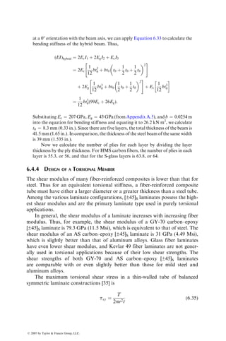
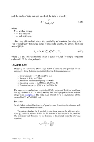
![differs from a pinned joint, since in the former the clamping torque is an
added factor contributing to the joint strength. The edge distance needed to
reduce shear-out failure can be reduced by increasing the laminate thickness at
the edge or by inserting metal shims between various composite layers near the
bolted area.
The strength of a mechanical joint can be improved significantly by reliev-
ing the stress concentrations surrounding the joint. The following are some of
the methods used for relieving stress concentrations.
Softening strips of lower modulus material are used in the bolt bearing area.
For example, strips made of E-glass fiber plies can be used to replace some of
the carbon fiber plies aligned with the loading direction in a carbon fiber-
reinforced laminate.
Laminate tailoring method [31] divides the bolt hole area of structure into two
regions, namely, a primary region and a bearing region. This is demonstrated
in Figure 6.12 for a structure made of a [02=±45]2S laminate. In the bearing
region surrounding the bolt hole, the 08 plies in the laminate are replaced by
±458 plies. Thus, the lower modulus bearing region is bounded on both sides
by the primary region of [02=±45] laminate containing 20%–60% 08 plies. The
majority of the axial load in the joint is carried by the high-modulus primary
region, which is free of fastener holes. The combination of low axial stress in
the bearing region and the relatively low notch sensitivity of the [±45] lamin-
ate delays the onset of the net tension failure commonly observed in non-
tailored [02=±45]S laminates.
(a) (b) (c) (d)
FIGURE 6.11 Basic failure modes in bolted laminates: (a) shear-out, (b) net tension
failure, (c) cleavage, and (d) bearing failure. Combinations of these failure modes are
possible.
ß 2007 by Taylor Francis Group, LLC.](https://image.slidesharecdn.com/fiberreinforcedcompositesmaterialsmanufacturinganddesignp1-220510152925-9ef3de0d/85/Fiber_Reinforced_Composites_Materials_Manufacturing_and_Design_P-1-pdf-521-320.jpg)
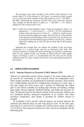
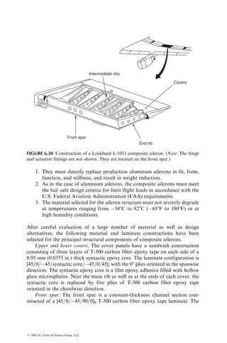
![stepped lap joint is used, it may often be easier and less expensive to lay up the
steps before cure. This eliminates the machining operation and prevents dam-
age to the fibers.
The following points are important in designing a bonded joint and select-
ing an appropriate adhesive for the joint.
1. Increasing the ratio of lap length to substrate thickness h improves the
joint strength significantly at small L=h ratios. At high L=h ratios, the
improvement is marginal (Figure 6.16).
2. Tapering the substrate ends at the ends of the overlap reduces the high
normal stresses at these locations [32].
3. Equal axial stiffnesses for the substrates are highly desirable for achiev-
ing the maximum joint strength (Figure 6.16). Since stiffness is a product
of modulus E and thickness h, it is important to select the proper
thickness of each substrate so that E1h1 ¼ E2h2. If the two substrates
are of the same material, their thicknesses must be equal.
4. The important characteristics of a good adhesive are high shear and
tensile strengths but low shear and tensile moduli. An efficient way of
Double lap
Aluminum
failure
Boron–epoxy to aluminum joints
(0/45/−45/0)
Adhesive: epoxy
Single lap
Scarf
S
t
e
p
p
e
d
l
a
p
Length of joint, L (in.)
Adhesive
joint
strength
(ksi)
14
12
10
6
4
2
0
0 0.5 1.0 1.5 2.0 2.5
8
FIGURE 6.15 Increase in the joint strength of single-lap bonded joints with lap length.
(After Griffin, O.H., Compos. Technol. Rev., 4, 136, 1982.)
ß 2007 by Taylor Francis Group, LLC.](https://image.slidesharecdn.com/fiberreinforcedcompositesmaterialsmanufacturinganddesignp1-220510152925-9ef3de0d/85/Fiber_Reinforced_Composites_Materials_Manufacturing_and_Design_P-1-pdf-524-320.jpg)
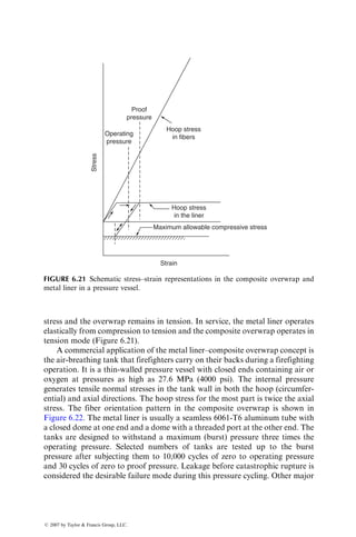
![For most 08 continuous fiber composites, the fatigue strength in tension–
tension cycling can be approximated as
S ¼ SLt(1 b log N), (6:23)
where the value of the constant b depends primarily on the fiber type
(Table 6.5). If the tension member is exposed to tension–tension fatigue, its
design should be based on the fatigue strength of the material at the desired
number of cycles. It should be noted that ranking of the fibers based on the
fatigue strength can be different from that based on the fiber tensile strength.
The most critical design issue for a tension member involves the joints or
connections at its ends. A few joint design ideas other than the simple bolted or
bonded joints are shown in Figure 6.18.
6.4.2 DESIGN OF A COMPRESSION MEMBER
Tubular compression members made from fiber-reinforced polymeric materials
are finding applications in many aerospace structures, such as satellite trusses,
support struts, and flight control rods. Since these compression members are
mostly slender tubes, their design is usually based on preventing overall column
buckling as well as local buckling [33].
The compressive stress on a thin tube of radius r and wall thickness t is
s ¼
P
A0
¼
P
2prt
, (6:24)
where P is the axial compressive load.
For a pin-ended column, the overall buckling stress is given by
scol ¼
2L2
p2Exxr2
þ
2
Gxy
1
, (6:25)
TABLE 6.5
Tensile Fatigue Strength Coefficient b for
Various 08 Laminates
Fiber Type b
Ultrahigh-modulus carbon 0.021
High-modulus carbon 0.035
High-strength carbon 0.05
Kevlar 49 0.035
S-glass 0.088
E-glass 0.093
ß 2007 by Taylor Francis Group, LLC.](https://image.slidesharecdn.com/fiberreinforcedcompositesmaterialsmanufacturinganddesignp1-220510152925-9ef3de0d/85/Fiber_Reinforced_Composites_Materials_Manufacturing_and_Design_P-1-pdf-527-320.jpg)
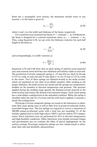
![Using Equations 6.24 through 6.26, Maass [33] developed the following
optimum stress equation for a compression tube design:
s3
opt
4
pExxb0(P=L2)
þ sopt
2
Gxy
¼ 1: (6:27)
Neglecting the shear term, an approximate sopt can be calculated as
sopt ¼
pExxb0(P=L2
)
4
1=3
, (6:28)
where (P=L2
) is called the loading index.
Knowing sopt from either Equation 6.27 or 6.28, the actual tube dimensions
can be determined from the following equations:
ropt ¼
Pb0
2ps2
opt
!
1=2
,
topt ¼
sopt
b0
ropt: (6:29)
Equations 6.27 through 6.29 show that the optimum design of a compression
tube depends very much on the laminate configuration. Maass [33] used these
equations to determine the optimum stress and the corresponding ply ratio for
various [0=±u]S tubes made of high-strength carbon–epoxy laminates. For a
unit loading index, the highest optimum stress occurs for a [03=±45]S tube,
although a [±15]S tube with no 08 fibers exhibits approximately the same
optimum stress. The optimum design with increasing off-axis angle u is
obtained with increasing percentages of 08 layers in the tube.
6.4.3 DESIGN OF A BEAM
Beams are slender structural members designed principally to resist transverse
loads. In general, the stress state at any point in the beam consists of an axial
normal stress sxx and a transverse shear stress txz. Both these stresses are
nonuniformly distributed across the thickness (depth) of the beam. In an
isotropic homogeneous beam, these stress distributions are continuous with
the maximum and minimum normal stresses occurring at the outermost surfaces
and the maximum shear stress occurring at the neutral axis. In laminated
beams, the normal stress and shear stress distributions are not only nonuniform,
but also they are discontinuous at the interfaces of dissimilar laminas.
Depending on the lamination configuration, it is possible to create maximum
normal stresses in the interior of the beam thickness and the maximum shear
ß 2007 by Taylor Francis Group, LLC.](https://image.slidesharecdn.com/fiberreinforcedcompositesmaterialsmanufacturinganddesignp1-220510152925-9ef3de0d/85/Fiber_Reinforced_Composites_Materials_Manufacturing_and_Design_P-1-pdf-529-320.jpg)
![stress away from the midplane of the beam. For this reason, the actual stress
distribution in a laminated composite beam should always be calculated using
the lamination theory instead of the homogeneous beam theory.
Except all 0, all 90, and 0=90 combinations for which D16 ¼ D26 ¼ 0, there
will be a bending–twisting coupling in all symmetric beams. This means that
a bending moment will create not only bending deformations, but also tend
to twist the beam. Whitney et al. [34] have shown that the deflection equation for
a symmetric beam has the same form as that for a homogeneous beam, namely,
d2
w
dx2
¼
bMxx
EbI
, (6:30)
where
w ¼ beam deflection
b ¼ beam width
Mxx ¼ bending moment per unit width
I ¼ moment of inertia of the cross section about the midplane
Eb ¼ effective bending modulus of the beam
The effective bending modulus Eb is defined as
Eb ¼
12
h3D11
*
, (6:31)
where
h is the beam thickness
D11
* is the first element in the inverse [D] matrix (see Example 3.13)
Equation 6.31 neglects the effect due to transverse shear, which can be
significant for beams with small span-to-thickness ratio. For long beams, for
which the effect of the transverse shear is negligible, the maximum deflection can
be calculated by replacing the isotropic modulus E with the effective bending
modulus Eb in the deflection formulas for homogeneous beams. From Equation
6.31, the effective bending stiffness for a laminated beam can be written as
EbI ¼
b
D11
*
: (6:32)
For a symmetric beam containing isotropic layers or specially orthotropic
layers (such as all 08, all 908, or combinations of 08 and 908 layers), the effective
bending stiffness becomes
(EI)b ¼ S(E11)jIj, (6:33)
ß 2007 by Taylor Francis Group, LLC.](https://image.slidesharecdn.com/fiberreinforcedcompositesmaterialsmanufacturinganddesignp1-220510152925-9ef3de0d/85/Fiber_Reinforced_Composites_Materials_Manufacturing_and_Design_P-1-pdf-530-320.jpg)
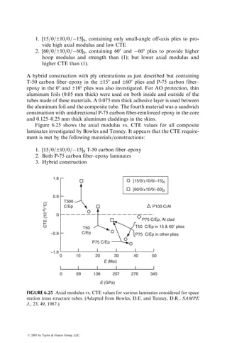
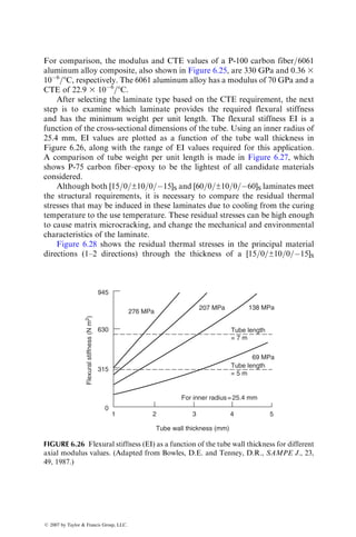
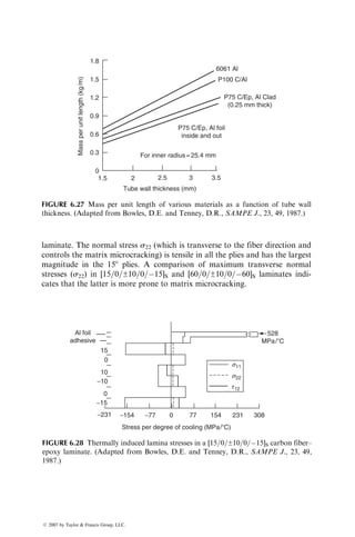
![at a 08 orientation with the beam axis, we can apply Equation 6.33 to calculate the
bending stiffness of the hybrid beam. Thus,
(EI)hybrid ¼ 2EcI1 þ 2EgI2 þ EcI3
¼ 2Ec
1
12
bt3
0 þ bt0 t0 þ
1
2
t0 þ
1
2
t0
2
#
þ 2Eg
1
12
bt3
0 þ bt0
1
2
t0 þ
1
2
t0
2
#
þ Ec
1
12
bt3
0
¼
1
12
bt3
0(99Ec þ 26Eg):
Substituting Ec ¼ 207 GPa, Eg ¼ 43 GPa (from Appendix A.5), and b ¼ 0.0254 m
into the equation for bending stiffness and equating it to 26.2 kN m2
, we calculate
t0 ¼ 8.3 mm (0.33 in.). Since there are five layers, the total thickness of the beam is
41.5 mm (1.65 in.). In comparison, the thickness of the steel beam of the same width
is 39 mm (1.535 in.).
Now we calculate the number of plies for each layer by dividing the layer
thickness by the ply thickness. For HMS carbon fibers, the number of plies in each
layer is 55.3, or 56, and that for the S-glass layers is 63.8, or 64.
6.4.4 DESIGN OF A TORSIONAL MEMBER
The shear modulus of many fiber-reinforced composites is lower than that for
steel. Thus for an equivalent torsional stiffness, a fiber-reinforced composite
tube must have either a larger diameter or a greater thickness than a steel tube.
Among the various laminate configurations, [±45]S laminates possess the high-
est shear modulus and are the primary laminate type used in purely torsional
applications.
In general, the shear modulus of a laminate increases with increasing fiber
modulus. Thus, for example, the shear modulus of a GY-70 carbon–epoxy
[±45]S laminate is 79.3 GPa (11.5 Msi), which is equivalent to that of steel. The
shear modulus of an AS carbon–epoxy [±45]S laminate is 31 GPa (4.49 Msi),
which is slightly better than that of aluminum alloys. Glass fiber laminates
have even lower shear modulus, and Kevlar 49 fiber laminates are not gener-
ally used in torsional applications because of their low shear strengths. The
shear strengths of both GY-70 and AS carbon–epoxy [±45]S laminates
are comparable with or even slightly better than those for mild steel and
aluminum alloys.
The maximum torsional shear stress in a thin-walled tube of balanced
symmetric laminate constructions [35] is
txy ¼
T
2pr2t
(6:35)
ß 2007 by Taylor Francis Group, LLC.](https://image.slidesharecdn.com/fiberreinforcedcompositesmaterialsmanufacturinganddesignp1-220510152925-9ef3de0d/85/Fiber_Reinforced_Composites_Materials_Manufacturing_and_Design_P-1-pdf-534-320.jpg)
![and the angle of twist per unit length of the tube is given by
f ¼
T
2pGxyr3t
, (6:36)
where
T ¼ applied torque
r ¼ mean radius
t ¼ wall thickness
For very thin-walled tubes, the possibility of torsional buckling exists.
For symmetrically laminated tubes of moderate lengths, the critical buckling
torque [36] is
Tcr ¼ 24:4CD
5=8
22 A
3=8
11 r5=4
L1=2
, (6:37)
where C is end-fixity coefficient, which is equal to 0.925 for simply supported
ends and 1.03 for clamped ends.
EXAMPLE 6.10
Design of an Automotive Drive Shaft. Select a laminate configuration for an
automotive drive shaft that meets the following design requirements:
1. Outer diameter ¼ 95.25 mm (3.75 in.)
2. Length ¼ 1.905 m (75 in.)
3. Minimum resonance frequency ¼ 90 Hz
4. Operating torque ¼ 2,822 N m (25,000 in. lb)
5. Overload torque ¼ 3,386 N m (30,000 in. lb)
Use a carbon–epoxy laminate containing 60% by volume of T-300 carbon fibers.
The ply thickness is 0.1524 mm (0.006 in.). The elastic properties of the material
are given in Example 3.6. The static shear strength for a [±45]S laminate of this
material is 455 MPa (66,000 psi).
SOLUTION
Step 1: Select an initial laminate configuration, and determine the minimum wall
thickness for the drive shaft.
The primary load on the drive shaft is a torsional moment for which we select
a [±45]kS laminate, where k stands for the number of ±458 layers in the laminate.
The minimum wall thickness for the laminate is determined from the following
equation:
tall ¼
Sxys
n
¼
Tmax
2pr2t
,
ß 2007 by Taylor Francis Group, LLC.](https://image.slidesharecdn.com/fiberreinforcedcompositesmaterialsmanufacturinganddesignp1-220510152925-9ef3de0d/85/Fiber_Reinforced_Composites_Materials_Manufacturing_and_Design_P-1-pdf-535-320.jpg)
![where
Tmax ¼ maximum torque ¼ 3386 N m
r ¼ mean radius ¼ 0.048 m
t ¼ wall thickness
Sxys ¼ static shear strength ¼ 455 3 106
N=m2
n ¼ factor of safety ¼ 2.2 (assumed)
Using this equation, we calculate t ¼ 0.001131 m ¼ 1.131 mm. Since each ply
is 0.1524 mm thick, the minimum number of 458 plies is (1.131=0.1524) ¼ 7.42.
Assume eight plies, so that the initial laminate configuration is [±45]2S.
Step 2: Check for the minimum resonance frequency. The fundamental resonance
frequency corresponding to the critical speed of a rotating shaft is
fcr ¼
1
2p
p2
L2
ffiffiffiffiffiffiffiffiffiffiffi
ExxIc
rA0
s
#
,
where
Exx ¼ axial modulus
A0 ¼ 2prt
Ic ¼ pr3
t
r ¼ density
Substituting for A0 and Ic, we obtain
fcr ¼
p
2
r
L2
ffiffiffiffiffiffiffiffi
Exx
2r
s
:
To meet the minimum resonance frequency, the shaft must have an adequate axial
modulus. Since the axial modulus of a [±45]2S laminate is rather low, we add four
plies of 08 layers to the previous ±458 layers so that the new laminate configur-
ation is [±45=02=±45]S. The two 458 layers are placed in the outer diameter instead
of the 08 layers to resist the maximum shear stress due to the torsional moment.
Using the lamination theory, we calculate Exx as 53.39 GPa. Since the ply material
contains 60% by volume of T-300 carbon fibers, its density is calculated as 1556
kg=m3
. Using these values, we calculate the resonance frequency as 86 Hz, which
is less than the minimum value required.
To improve the resonance frequency, we add two more layers of 08 plies,
which brings the laminate configuration to [±45=03=±45]S. Using the lamination
theory, we recalculate Exx as 65.10 GPa. The resonance frequency of this new
shaft is 95 Hz, which exceeds the minimum value required.
Step 3: Check for the maximum torsional shear stress. We need to check for
the maximum torsional shear stress since the laminate configuration is
different from that assumed in Step 1. The [±45=03=±45]S laminate
contains 14 plies with a wall thickness of 14 3 0.1524 mm ¼ 2.13 mm.
The maximum torsional shear stress is calculated as 109.8 MPa.
ß 2007 by Taylor Francis Group, LLC.](https://image.slidesharecdn.com/fiberreinforcedcompositesmaterialsmanufacturinganddesignp1-220510152925-9ef3de0d/85/Fiber_Reinforced_Composites_Materials_Manufacturing_and_Design_P-1-pdf-536-320.jpg)
![The maximum static shear strength of the [±45=03=±45]S laminate is not
known. Since 57% of this laminate is ±458 layers, we estimate its shear strength
as 57% of the static shear strength of the [±45]S laminate, or 0.57 3 455 MPa ¼
260 MPa. Comparing the maximum torsional shear stress with this estimated
shear strength, we find the factor of safety as n ¼ 260=109.8 ¼ 2.37, which is
adequate for the torsional shear stress.
Step 4: Check the critical buckling torque. Using the lamination theory, we
calculate D22 ¼ 71.48 N m and A11 ¼ 1714.59 3 105
N=m. Substitution
of these values into Equation 6.37 gives Tcr ¼ 6420 N m, which is nearly
twice the maximum application torque. Thus the [±45=03=±45]S laminate
is safe against torsional buckling. If this were not the case, the easiest way
to increase the critical buckling torque would be to increase D22, which is
achieved by adding one or more 908 plies on both sides of the laminate
midplane.
Although this example does not address the problem of the end fitting
attachments, it is a critical design issue for an automotive drive shaft. The
common methods of attaching the metal end fittings are bonded or interference
joints for low applied torques and bonded or bolted joints for high applied
torques. If bolting is used, it is recommended that the joint area be locally
reinforced either by using a tubular metal insert or by using additional layers in
the laminate.
6.5 APPLICATION EXAMPLES
6.5.1 INBOARD AILERONS ON LOCKHEED L-1011 AIRCRAFT [37]
Ailerons are adjustable control surfaces hinged to the wing trailing edges of
an aircraft for controlling its roll (rotation about the longitudinal axis).
Their angular positions are manipulated by hydraulic actuators. Each aileron
has a wedge-shaped one-cell box configuration consisting of a front spar, a
rear spar, upper and lower covers, and a number of reinforcing ribs. Other
parts in the aileron assembly are leading edge shrouds, end fairings, trailing
edge wedge, shroud supports, feedback fittings, and hinge and actuator fit-
tings. The primary load on the aileron surfaces is the air pressure. Ailerons are
not considered primary structural components in an aircraft. Like other
secondary components, their design is governed by stiffness instead of
strength.
In Lockheed L-1011 aircraft, inboard ailerons are located between the
outboard and inboard flaps on each wing (Figure 6.20). At the front spar,
each aileron is 2.34 m (92 in.) in length and ~250 mm (10 in.) deep. Its width is
1.27 m (50 in.). The composite ailerons in L-1011 aircraft are designed with the
following goals.
ß 2007 by Taylor Francis Group, LLC.](https://image.slidesharecdn.com/fiberreinforcedcompositesmaterialsmanufacturinganddesignp1-220510152925-9ef3de0d/85/Fiber_Reinforced_Composites_Materials_Manufacturing_and_Design_P-1-pdf-537-320.jpg)
![1. They must directly replace production aluminum ailerons in fit, form,
function, and stiffness, and result in weight reduction.
2. As in the case of aluminum ailerons, the composite ailerons must meet
the fail–safe design criteria for limit flight loads in accordance with the
U.S. Federal Aviation Administration (FAA) requirements.
3. The material selected for the aileron structure must not severely degrade
at temperatures ranging from 548C to 828C (658F to 1808F) or at
high humidity conditions.
After careful evaluation of a large number of material as well as design
alternatives, the following material and laminate constructions have been
selected for the principal structural components of composite ailerons.
Upper and lower covers: The cover panels have a sandwich construction
consisting of three layers of T-300 carbon fiber–epoxy tape on each side of a
0.95 mm (0.0375 in.) thick syntactic epoxy core. The laminate configuration is
[45=0=45=syntactic core=45=0=45], with the 08 plies oriented in the spanwise
direction. The syntactic epoxy core is a film epoxy adhesive filled with hollow
glass microspheres. Near the main rib as well as at the ends of each cover, the
syntactic core is replaced by five plies of T-300 carbon fiber–epoxy tape
oriented in the chordwise direction.
Front spar: The front spar is a constant-thickness channel section con-
structed of a [45=0=45=90=0]S T-300 carbon fiber–epoxy tape laminate. The
Intermediate ribs
Covers
Front spar
End rib
FIGURE 6.20 Construction of a Lockheed L-1011 composite aileron. (Note: The hinge
and actuator fittings are not shown. They are located on the front spar.)
ß 2007 by Taylor Francis Group, LLC.](https://image.slidesharecdn.com/fiberreinforcedcompositesmaterialsmanufacturinganddesignp1-220510152925-9ef3de0d/85/Fiber_Reinforced_Composites_Materials_Manufacturing_and_Design_P-1-pdf-538-320.jpg)
![08 plies in the front spar laminate are in the spanwise direction. Holes are
machined in the spar web for access and inspection purposes. The flange
width of the spar caps is increased locally to facilitate mountings of main ribs
and rib backup fittings.
Main ribs: Main ribs are used at three hinge or actuator fitting locations for
transferring loads from the fittings to the aileron covers and spars. They are
constant-thickness channel sections constructed with four plies of T-300 carbon
fiber–epoxy bidirectional fabric oriented at [45=902=45], where 08 represents the
lengthwise direction for the rib. Five plies of unidirectional 08 T-300 carbon
fiber–epoxy tape are added to the rib cap to increase the stiffness and strength
at the rib ends.
Other ribs: In addition to the three main ribs, the aileron assembly has five
intermediate ribs and two end closeout ribs that support the covers and share
the air pressure load. These ribs are constant-thickness channel sections con-
sisting of five plies of T-300 carbon fiber–epoxy bidirectional fabric oriented at
[45=90=45=90=45], where the 08 direction represents the lengthwise direction
for each rib. Five holes are machined in each rib to reduce its weight.
Rear spar: No material substitution is made for the rear spar, since the
usage of composites is considered too expensive for the small amount of weight
saved over the existing constant-thickness channel section of 7075-T6 clad
aluminum.
In the aileron assembly, the upper cover, all ribs, and two spars are perman-
ently fastened with titanium screws and stainless steel collars. The removable
lower cover, trailing edge wedge, leading edge shroud, and fairings are fastened
with the same type of screws, but with stainless steel nut plates attached to these
substructures with stainless steel rivets. To prevent galvanic corrosion, all alu-
minum parts are anodized, primed with epoxy, and then painted with a urethane
top coat. All carbon fiber–epoxy parts are also painted with a urethane coat.
The composite aileron is 23.2% lighter than the metal aileron. It also
contains 50% fewer parts and fasteners (Table 6.7). A summary of the ground
TABLE 6.7
Comparison of Composite and Metal Ailerons
Composite Aluminum
Weight (lb) 100.1 140.4
Number of ribs 10 18
Number of parts 205 398
Number of fasteners 2574 5253
Source: Adapted from Griffin, C.F., Design development of an
advanced composite aileron, Paper No. 79–1807, AIAA Aircraft
Systems and Technology Meeting, August 1979.
ß 2007 by Taylor Francis Group, LLC.](https://image.slidesharecdn.com/fiberreinforcedcompositesmaterialsmanufacturinganddesignp1-220510152925-9ef3de0d/85/Fiber_Reinforced_Composites_Materials_Manufacturing_and_Design_P-1-pdf-539-320.jpg)
![tests performed on the aileron assemblies is given in Table 6.8. Additionally, a
number of composite aileron prototypes have also been tested on the aircraft
during engine run-up, level flights, and high-speed descends. The performance
of composite aileron prototypes has been judged equal to or better than the
performance of metal ailerons in these tests. As part of the maintenance
evaluation program, five sets of composite ailerons were installed on commer-
cial aircrafts and placed in service in September 1981.
6.5.2 COMPOSITE PRESSURE VESSELS [38]
Composite pressure vessels with S-glass or Kevlar 49 fiber-reinforced epoxy
wrapped around a metal liner are used in many space, military, and commercial
applications. The liner is used to prevent leakage of the high-pressure fluid
through the matrix microcracks that often form in the walls of filament-wound
fiber-reinforced epoxy pressure vessels. The winding is done on the liner, which
also serves as a mandrel. The winding tension and the subsequent curing action
create compressive stresses in the liner and tensile stresses in the fiber-
reinforced epoxy overwrap. After fabrication, each vessel is pressurized with
an internal proof pressure (also called the ‘‘sizing’’ pressure) to create tensile
yielding in the metal liner and additional tensile stresses in the overwrap. When
the proof pressure is released, the metal liner attains a compressive residual
TABLE 6.8
Ground Tests on Lockheed L-1011 Composite Ailerons
Vibration in the flapping mode Resonance frequencies comparable with those
of metal ailerons
Vibration in the torsional mode Resonance frequencies comparable with those
of metal ailerons
Chordwise static bending stiffness Composite ailerons 27% less stiff than metal
ailerons
Static torsional stiffness Comparable with metal ailerons
Static loading 124% Design ultimate load without failure at 128
down-aileron positions
139% Design ultimate load at 208 up-aileron
positions with postbuckling of the hinge and
backup rib webs
Impact loading to cause visible damage at
four locations followed by one lifetime
flight-by-flight fatigue loading
Slight growth of damage (caused by impact
loading) during the fatigue cycling
Simulated lightning followed by static
loading
Burn-through and delamination over a small
area; however, no evidence of growth of this
damage during static testing
Source: Adapted from Griffin, C.F., Design development of an advanced composite aileron, Paper
No. 79–1807, AIAA Aircraft Systems and Technology Meeting, August 1979.
ß 2007 by Taylor Francis Group, LLC.](https://image.slidesharecdn.com/fiberreinforcedcompositesmaterialsmanufacturinganddesignp1-220510152925-9ef3de0d/85/Fiber_Reinforced_Composites_Materials_Manufacturing_and_Design_P-1-pdf-540-320.jpg)
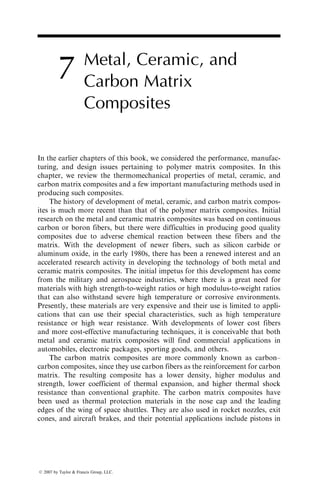
![qualification tests for the air-breathing tanks are drop impacts, exposure to
high temperatures in the pressurized condition, and exposure to direct fire.
6.5.3 CORVETTE LEAF SPRINGS [39]
The first production application of fiber-reinforced polymers in an automotive
structural component is the 1981 Corvette leaf spring manufactured by the
General Motors Corporation. It is a single-leaf transverse spring weighing
about 35.3 N (7.95 lb) that directly replaces a 10-leaf spring weighing 182.5 N
(41 lb).
The material in the 1981 Corvette composite spring is an E-glass fiber-
reinforced epoxy with fibers oriented parallel to the length direction of the
spring. Although the cross-sectional area of the spring is uniform, its width and
thickness are varied to achieve a constant stress level along its length. This
design concept can be easily understood by modeling the spring as a simply
supported straight beam with a central vertical load P (Figure 6.23). If the
Longitudinal
wrap
Hoop
wrap
Metal liner
Longitudinal fibers
Circumferential fibers
a
FIGURE 6.22 Fiber orientation in the composite overwrap of a pressure vessel.
Section A-A
t
A
A
P
x
L
2
L
2
b
FIGURE 6.23 Simplified model of a leaf spring.
ß 2007 by Taylor Francis Group, LLC.](https://image.slidesharecdn.com/fiberreinforcedcompositesmaterialsmanufacturinganddesignp1-220510152925-9ef3de0d/85/Fiber_Reinforced_Composites_Materials_Manufacturing_and_Design_P-1-pdf-542-320.jpg)

![Figure 6.24 shows photographs of 1984 Corvette front and rear springs
made of E-glass–epoxy composite material. The front spring has a constant
width, but the rear spring has a variable width. Both springs are transversely
mounted in the car. At maximum wheel travel, the front and rear springs
support 13,000 N (2,925 lb.) and 12,000 N (2,700 lb.), respectively.
6.5.4 TUBES FOR SPACE STATION TRUSS STRUCTURE [40]
The truss structure in low earth orbiting (LEO) space stations is made of
tubular members with a nominal diameter of 50 mm (2 in.). Lengths of these
tubes are 7 m (23 ft.) for the diagonal members and 5 m (16.4 ft.) for other
members. The function of the truss structure is to support the crew and lab
modules as well as the solar arrays.
The important design criteria for the tubes are
1. Maximum axial load ¼ ±5.33 kN (±1200 lb.)
2. Coefficient of thermal expansion ¼ 0 ± 0.9 3 106
=8C (CTE in the axial
direction including the end fittings)
3. Low outgassing
4. Joints that allow easy tube replacements while in operation
5. 30 year service life
In addition, there are several environmental concerns in using polymer matrix
composites for the space station applications:
FIGURE 6.24 E glass–epoxy front (top) and rear (bottom) springs for 1984 Corvette.
(Courtesy of General Motors Corporation.)
ß 2007 by Taylor Francis Group, LLC.](https://image.slidesharecdn.com/fiberreinforcedcompositesmaterialsmanufacturinganddesignp1-220510152925-9ef3de0d/85/Fiber_Reinforced_Composites_Materials_Manufacturing_and_Design_P-1-pdf-544-320.jpg)
![1. Atomic oxygen (AO) degradation: Atomic oxygen is the major compon-
ent in the LEO atmosphere. On prolonged exposure, it can substantially
reduce the thickness of carbon fiber-reinforced epoxy tubes and reduce
their properties. The AO degradation of such tubes can be controlled by
wrapping them with a thin aluminum foil or by cladding them with an
aluminum layer.
2. Damage due to thermal cycling: It is estimated that the space station,
orbiting at 250 nautical miles with an orbital period of 90 min, will
experience 175,000 thermal cyclings during a 30 year service life. Unless
protected by reflective aluminum coatings, the transient temperature
variation may range from 628C to 778C. In the ‘‘worst case’’ situation,
for example, when the tube is always shadowed, the lowest steady-state
temperature may reach 1018C.
3. Damage due to low-velocity impact during assembly or due to extravehi-
cular activities. This type of damage may occur when two tubes acciden-
tally strike one another or when a piece of equipment strikes the tube.
These incidents can cause internal damages in the tube material and
reduce its structural properties. They can also damage the AO protective
coating and expose the tube material to atomic oxygen.
Since the tubes have large slenderness ratios (length-to-diameter ratios) and are
subjected to axial loading, column buckling is considered to be the primary
failure mode. Using Euler’s buckling formula for pin-ended columns, the
critical axial force is written as
Pcr ¼
p2
EI
L2
, (6:41)
where
E ¼ axial modulus for the tube material
I ¼ moment of inertia of the tube cross section
L ¼ tube length
Setting Pcr ¼ 5.33 kN, the minimum allowable flexural stiffness (EI) is
calculated as 26.49 kN m2
for the 7 m long diagonal tubes and 13.51 kN m2
for
the 5 m long nondiagonal tubes.
The CTE requirement for the entire tube including its end fittings is 0 ± 0.9 3
106
=8C. Assuming that the end fittings are made of aluminum and are 5% of the
total length, the CTE requirement for the tube is 0.635 ± 0.5 3 106
=8C.
Bowles and Tenney [40] used the lamination theory to calculate the axial
modulus (E) and CTE for several carbon fiber-reinforced composites. The first
three composites are 1778C (3508F) cure carbon fiber–epoxies containing either
T-300, T-50, or P-75 carbon fibers (having Ef ¼ 207, 344.5, and 517 GPa,
respectively). Two different ply orientations were examined for each of these
material systems:
ß 2007 by Taylor Francis Group, LLC.](https://image.slidesharecdn.com/fiberreinforcedcompositesmaterialsmanufacturinganddesignp1-220510152925-9ef3de0d/85/Fiber_Reinforced_Composites_Materials_Manufacturing_and_Design_P-1-pdf-545-320.jpg)
![1. [15=0=±10=0=15]S, containing only small-angle off-axis plies to pro-
vide high axial modulus and low CTE
2. [60=0=±10=0=60]S, containing 608 and 608 plies to provide higher
hoop modulus and strength than (1); but lower axial modulus and
higher CTE than (1).
A hybrid construction with ply orientations as just described but containing
T-50 carbon fiber–epoxy in the ±158 and ±608 plies and P-75 carbon fiber–
epoxy in the 08 and ±108 plies was also investigated. For AO protection, thin
aluminum foils (0.05 mm thick) were used on both inside and outside of the
tubes made of these materials. A 0.075 mm thick adhesive layer is used between
the aluminum foil and the composite tube. The fourth material was a sandwich
construction with unidirectional P-75 carbon fiber-reinforced epoxy in the core
and 0.125–0.25 mm thick aluminum claddings in the skins.
Figure 6.25 shows the axial modulus vs. CTE values for all composite
laminates investigated by Bowles and Tenney. It appears that the CTE require-
ment is met by the following materials=constructions:
1. [15=0=±10=0=15]S T-50 carbon fiber–epoxy
2. Both P-75 carbon fiber–epoxy laminates
3. Hybrid construction
CTE
(10
−6
/
⬚C)
E (GPa)
E (Msi)
0.9
1.8
0
−1.8
0
0 138
69 207 276 345
10 20 30 40 50
−0.9
T50
C/Ep
P75 C/Ep
T50 C/Ep in 15 60⬚ plies
P75 C/Ep in other plies
P75 C/Ep, Al clad
P100 C/Al
T300
C/Ep
[15/0/±10/0/−15]S
[60/0/±10/0/−60]S
FIGURE 6.25 Axial modulus vs. CTE values for various laminates considered for space
station truss structure tubes. (Adapted from Bowles, D.E. and Tenney, D.R., SAMPE
J., 23, 49, 1987.)
ß 2007 by Taylor Francis Group, LLC.](https://image.slidesharecdn.com/fiberreinforcedcompositesmaterialsmanufacturinganddesignp1-220510152925-9ef3de0d/85/Fiber_Reinforced_Composites_Materials_Manufacturing_and_Design_P-1-pdf-546-320.jpg)
![For comparison, the modulus and CTE values of a P-100 carbon fiber=6061
aluminum alloy composite, also shown in Figure 6.25, are 330 GPa and 0.36 3
106
=8C, respectively. The 6061 aluminum alloy has a modulus of 70 GPa and a
CTE of 22.9 3 106
=8C.
After selecting the laminate type based on the CTE requirement, the next
step is to examine which laminate provides the required flexural stiffness
and has the minimum weight per unit length. The flexural stiffness EI is a
function of the cross-sectional dimensions of the tube. Using an inner radius of
25.4 mm, EI values are plotted as a function of the tube wall thickness in
Figure 6.26, along with the range of EI values required for this application.
A comparison of tube weight per unit length is made in Figure 6.27, which
shows P-75 carbon fiber–epoxy to be the lightest of all candidate materials
considered.
Although both [15=0=±10=0=15]S and [60=0=±10=0=60]S laminates meet
the structural requirements, it is necessary to compare the residual thermal
stresses that may be induced in these laminates due to cooling from the curing
temperature to the use temperature. These residual stresses can be high enough
to cause matrix microcracking, and change the mechanical and environmental
characteristics of the laminate.
Figure 6.28 shows the residual thermal stresses in the principal material
directions (1–2 directions) through the thickness of a [15=0=±10=0=15]S
Flexural
stiffness
(N
m
2
)
945
630
315
0
Tube wall thickness (mm)
1 2 3 4 5
276 MPa
For inner radius=25.4 mm
Tube length
= 5 m
Tube length
= 7 m
138 MPa
69 MPa
207 MPa
FIGURE 6.26 Flexural stiffness (EI) as a function of the tube wall thickness for different
axial modulus values. (Adapted from Bowles, D.E. and Tenney, D.R., SAMPE J., 23,
49, 1987.)
ß 2007 by Taylor Francis Group, LLC.](https://image.slidesharecdn.com/fiberreinforcedcompositesmaterialsmanufacturinganddesignp1-220510152925-9ef3de0d/85/Fiber_Reinforced_Composites_Materials_Manufacturing_and_Design_P-1-pdf-547-320.jpg)
![laminate. The normal stress s22 (which is transverse to the fiber direction and
controls the matrix microcracking) is tensile in all the plies and has the largest
magnitude in the 158 plies. A comparison of maximum transverse normal
stresses (s22) in [15=0=±10=0=15]S and [60=0=±10=0=60]S laminates indi-
cates that the latter is more prone to matrix microcracking.
For inner radius=25.4 mm
P75 C/Ep, Al foil
inside and out
6061 Al
P100 C/Al
P75 C/Ep, Al Clad
(0.25 mm thick)
Tube wall thickness (mm)
Mass
per
unit
length
(kg
/m)
1.8
1.5
1.2
0.9
0.6
0.3
0
1.5 2 2.5 3 3.5
FIGURE 6.27 Mass per unit length of various materials as a function of tube wall
thickness. (Adapted from Bowles, D.E. and Tenney, D.R., SAMPE J., 23, 49, 1987.)
0 77
−77 154
−154 231
−231
−15
0
0
15
Al foil
adhesive
Stress per degree of cooling (MPa/⬚C)
528
MPa/⬚C
10
−10
308
s11
s22
t12
FIGURE 6.28 Thermally induced lamina stresses in a [15=0=±10=0=15]S carbon fiber–
epoxy laminate. (Adapted from Bowles, D.E. and Tenney, D.R., SAMPE J., 23, 49,
1987.)
ß 2007 by Taylor Francis Group, LLC.](https://image.slidesharecdn.com/fiberreinforcedcompositesmaterialsmanufacturinganddesignp1-220510152925-9ef3de0d/85/Fiber_Reinforced_Composites_Materials_Manufacturing_and_Design_P-1-pdf-548-320.jpg)
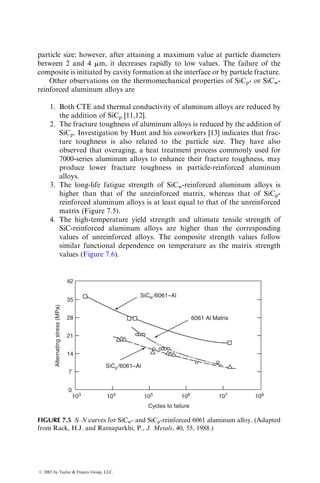
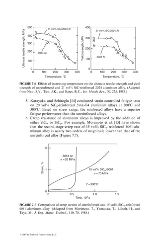
![PROBLEMS
P6.1. A Kevlar 49–epoxy composite has the following material properties:
E11 ¼ 11 3 106
psi, E22 ¼ 0.8 3 106
psi, G12 ¼ 0.33 3 106
psi, n12 ¼
0.34, SLt ¼ 203 ksi, STt ¼ 1.74 ksi, SLc ¼ 34 ksi, STc ¼ 7.7 ksi, and
SLTs ¼ 4.93 ksi. A unidirectional laminate of this material is subjected to
uniaxial tensile loading in the x direction. Determine the failure stress of
the laminate using (a) the maximum stress theory, (b) the maximum strain
theory, and (c) the Azzi–Tsai–Hill theory for u ¼ 08, 308, 458, 608, and 908.
P6.2. The Kevlar 49–epoxy composite in Problem P6.1 has a fiber orientation
angle of 458 and is subjected to a biaxial normal stress field (txy ¼ 0).
Determine the failure stress of the laminate using (a) the maximum stress
theory, (b) the maximum strain theory, and (c) the Azzi–Tsai–Hill theory
for the normal stress ratios of 0, 1, and 2.
P6.3. Biaxial tension–compression tests on closed-ended 908 tubes (with fibers
oriented in the hoop direction of the tube) are performed to determine
the normal stress interaction parameter F12, which appears in the Tsai–
Wu failure criterion.
The desired stress state is created by a combination of the internal
pressure and axial compressive load. In one particular experiment with
carbon fiber–epoxy composites, the biaxial stress ratio s11=s22 was 9.
The internal tube diameter was 2 in. and the tube wall thickness was 0.05
in. If the burst pressure was recorded as 2700 psi, determine (a) the axial
compressive load at the time of failure and (b) the value of F12 for this
carbon fiber–epoxy composite.
The following strength properties for the material are known:
SLt ¼ 185ksi,STt ¼ 7.5ksi,SLc ¼ 127ksi,STc ¼ 34ksi,andSLTs ¼ 11ksi.
P6.4. Average tensile strengths of 158, 458, and 608 boron–epoxy off-axis tensile
specimens are 33.55, 12.31, and 9.28 ksi, respectively. Determine F12 for
these three cases using the Tsai–Wu failure theory. Which of the three F12
values is in the permissible range? What conclusion can be made about the
use of an off-axis tensile test for determining the F12 value? The following
properties are known for the boron–epoxy system: SLt ¼ 188 ksi, SLc ¼
361 ksi, STt ¼ 9 ksi, STc ¼ 45 ksi, and SLTs ¼ 10 ksi.
P6.5. A [0=45]8S T-300 carbon fiber–epoxy laminate is subjected to a uniaxial
tensile force Fxx.
Each ply in this laminate is 0.1 mm thick. The laminate is 100 mm
wide. The ply-level elastic properties of the material are given in Example
3.6. The basic strength properties of the material are as follows:
ß 2007 by Taylor Francis Group, LLC.](https://image.slidesharecdn.com/fiberreinforcedcompositesmaterialsmanufacturinganddesignp1-220510152925-9ef3de0d/85/Fiber_Reinforced_Composites_Materials_Manufacturing_and_Design_P-1-pdf-551-320.jpg)
![SLt ¼ SLc ¼ 1447.5 MPa, STt ¼ STc ¼ 44.8 MPa, and SLTs ¼ 62
MPa. Assuming that the maximum stress failure theory applies to this
material, determine Fxx at (a) FPF and (b) ultimate failure.
P6.6. A [0=90=±45]S T-300 carbon fiber–epoxy laminate is subjected to the
following in-plane loads: Nxx ¼ 1000 lb=in., Nyy ¼ 200 lb=in., and
Nxy ¼ 500 lb=in. Each ply in the cured laminate is 0.006 in. thick.
The basic elastic and ultimate properties of the material are as follows:
E11 ¼ 20 3 106
psi, E22 ¼ 1.3 3 106
psi, G12 ¼ 1.03 3 106
psi, n12 ¼ 0.3,
«Lt ¼ 0.0085, «Lc ¼ 0.0098, «Tt ¼ 0.0045, «Tc ¼ 0.0090, and gLTs ¼
0.015. Using the maximum strain theory, determine whether any of the
laminas in this laminate would fail at the specified load.
P6.7. If the laminate in Problem P6.6 is subjected to an increasing unaxial
load in the x direction, determine the minimum load at which the FPF
would occur.
P6.8. Show that, for an isotropic material, Equation 6.8 gives a hole stress
concentration factor of 3.
P6.9. Show that the hole stress concentration factor for a 08 laminate is
KT ¼ 1 þ
ffiffiffiffiffiffiffiffiffiffiffiffiffiffiffiffiffiffiffiffiffiffiffiffiffiffiffiffiffiffiffiffiffiffiffiffiffiffiffiffiffiffiffiffiffiffi
2
ffiffiffiffiffiffiffi
E11
E22
r
n12
þ
E11
G12
s
:
P6.10. Compare the hole stress concentration factors of [0=90]4S, [0=90=±45]2S,
and [0=90=±60]2S T-300 carbon fiber–epoxy laminates. The basic lam-
ina properties are: E11 ¼ 21 3 106
psi, E22 ¼ 1.35 3 106
psi, n12 ¼
0.25, and G12 ¼ 0.83 3 106
psi.
P6.11. A 10 mm diameter hole is drilled at the center of the 100 mm wide
[0=45]8S laminate in Problem P6.5. Calculate the hole stress concentra-
tion factor of the laminate, and state how it may change if (a) some of
the 458 layers are replaced with 458 layers, (b) some of the 458 layers
are replaced with 908 layers, and (c) some of the 458 layers are replaced
with 08 layers.
P6.12. Using the point stress criterion, estimate the notched tensile strength
of a [0=±30=90]8S T-300 carbon fiber–epoxy laminate containing a
central hole of (a) 0.25 in. diameter and (b) 1 in. diameter. Assume
that the characteristic distance d0 for the material is 0.04 in. The basic
elastic properties for the material are given in Problem P6.10. Assume
sUt ¼ 61 ksi.
ß 2007 by Taylor Francis Group, LLC.](https://image.slidesharecdn.com/fiberreinforcedcompositesmaterialsmanufacturinganddesignp1-220510152925-9ef3de0d/85/Fiber_Reinforced_Composites_Materials_Manufacturing_and_Design_P-1-pdf-552-320.jpg)
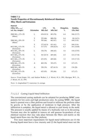
![outside layers. Assuming that the plate is pinned along its width,
determine the minimum number of 08 and 908 plies required to avoid
failure due to buckling. Each cured layer in the laminate is 0.125 mm
thick. Basic elastic properties of the material are given in Appendix A.5.
P6.17. A 20 in. long E-glass–polyester pultruded rod (vf ¼ 50%) with a solid
round cross section is designed to carry a static tensile load of 1000 lb.
The longitudinal extension of the rod may not exceed 0.05 in. Deter-
mine the minimum diameter of the rod. Laboratory tests have shown
that the tensile strength and tensile modulus for the material is 100,000
psi and 5.5 3 106
psi, respectively. Assume a factor of safety of 2.0.
P6.18. A 1 m tension bar of solid round cross section is to be designed using
unidirectional GY-70 carbon fiber-reinforced epoxy with 60% fiber
volume fraction. The maximum load on the rod is expected to be 445
kN. The rod may be subjected to tension–tension fatigue cycling at an
average cycling rate of 10 cycles=s for a total time period of 10 years in
an environment where the temperature may fluctuate between 208C
and 1008C. The elongation of the rod should not exceed 0.2 mm.
1. Determine the diameter of the rod using a factor of safety of 3.
2. Assume the rod will be pin-connected at each end to another struc-
ture, propose two conceptual designs for the end fittings for the rod
and discuss their applicability.
P6.19. A [0=±45=90]4S T-300 carbon fiber–epoxy laminate is used in a beam
application. Each layer in the cured laminate is 0.005 in. thick. The
beam is 0.5 in. wide. Using the basic elastic properties in Problem P6.10,
calculate the effective bending stiffness of the laminated beam.
P6.20. Determine the effective bending stiffness and the failure load of a
[(0=90)8=0]S E-glass–epoxy beam having a rectangular cross section,
12.7 mm wide 3 4.83 mm thick. Assume that each layer in the beam
has the same cured thickness. Use Appendix A.5 for the basic material
properties.
P6.21. A cantilever beam, 0.1 m long 3 50 mm wide 3 10 mm thick, has a
sandwich construction with [0=±45=90]S carbon fiber–epoxy facings
and an aluminum honeycomb core. Each layer in the cured laminate
is 0.125 mm thick. Assuming that the core has a negligible bending
stiffness, determine the end deflection of the beam if it is subjected to a
2000 N load at its free end. Basic ply-level elastic properties of the
material are the same as in Example 3.6.
ß 2007 by Taylor Francis Group, LLC.](https://image.slidesharecdn.com/fiberreinforcedcompositesmaterialsmanufacturinganddesignp1-220510152925-9ef3de0d/85/Fiber_Reinforced_Composites_Materials_Manufacturing_and_Design_P-1-pdf-554-320.jpg)
![P6.22. A 2 m long, 100 mm wide, simply supported rectangular beam is
subjected to a central load of 5 kN. The beam material is pultruded
E-glass–polyester containing 60 wt% continuous fibers and 20 wt% mat.
Determine the thickness of the beam so that its central deflection does
not exceed 70 mm. Laboratory tests have shown that the tensile modu-
lus of the material is 35.2 GPa. Assume its flexural modulus to be 20%
less than the tensile modulus.
P6.23. A 30 in. long automotive transmission member has a hat section with
uniform thickness. It is connected to the frame by means of two bolts at
each end. The maximum load acting at the center of the member is
estimated not to exceed 600 lb during its service life. The material
considered for its construction is SMC-C20R30.
Modeling the transmission member as a simply supported beam,
determine its thickness and the maximum deflection at its center. What
special attention must be given at the ends of the transmission member
where it is bolted to the frame? The fatigue strength of the SMC
material at 106
cycles is 45% of its static tensile strength.
P6.24. Using the same material and design requirements as in Example 6.10,
design the wall thickness of an automotive drive shaft with a [±15]nS
T-300 carbon fiber–epoxy laminate.
P6.25. Design a constant stress cantilever leaf spring of uniform width (70 mm)
using (a) E-glass–epoxy and (b) AS carbon–epoxy. Free length of the
spring is 500 mm. It is subjected to a reversed fatigue load of ±10 kN.
What will be a suitable manufacturing method for this spring?
ß 2007 by Taylor Francis Group, LLC.](https://image.slidesharecdn.com/fiberreinforcedcompositesmaterialsmanufacturinganddesignp1-220510152925-9ef3de0d/85/Fiber_Reinforced_Composites_Materials_Manufacturing_and_Design_P-1-pdf-555-320.jpg)
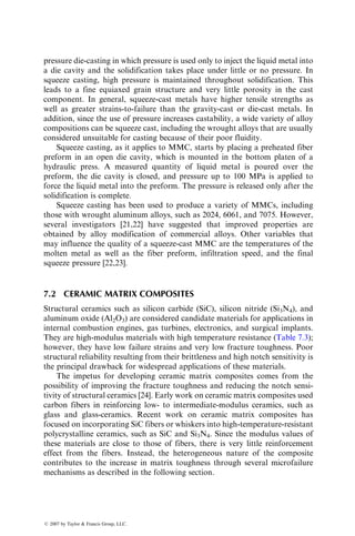
![internal combustion engines, gas turbine components, heat exchangers, and
biomedical implants.
7.1 METAL MATRIX COMPOSITES
The metal matrix composites (MMC) can be divided into four general categories:
1. Fiber-reinforced MMC containing either continuous or discontinuous
fiber reinforcements; the latter are in the form of whiskers with approxi-
mately 0.10.5 mm in diameter and have a length-to-diameter ratio up
to 200.
2. Particulate-reinforced MMC containing either particles or platelets that
range in size from 0.5 to 100 mm. The particulates can be incorporated
into the metal matrix to higher volume fractions than the whiskers.
3. Dispersion-strengthened MMC containing particles that are 0.1 mm in
diameter.
4. In situ MMC, such as directionally solidified eutectic alloys.
In this chapter, we focus our attention on the first two categories, more
specifically on whisker- and particulate-reinforced MMCs. More detailed infor-
mations on MMC can be found in Refs. [1–4].
Continuous carbon or boron fiber-reinforced MMCs have been under
development for 20 years; however, they have found limited use due to
problems in controlling the chemical reaction between the fibers and the molten
metal at the high processing temperatures used for such composites. The result
of this chemical reaction is a brittle interphase that reduces the mechanical
properties of the composite. Fiber surface treatments developed to reduce this
problem increase the cost of the fiber. Additionally, the manufacturing cost of
continuous carbon or boron fiber-reinforced MMC is also high, which makes
them less attractive for many applications. Much of the recent work on MMC
is based on silicon carbide whiskers (SiCw) or silicon carbide particulates
(SiCp). SiC is less prone to oxidative reactions at the processing temperatures
used. Furthermore, not only they are less expensive than carbon or boron
fibers, but also they can be incorporated into metal matrices using common
manufacturing techniques, such as powder metallurgy and casting.
7.1.1 MECHANICAL PROPERTIES
In Chapter 2, we discussed simple micromechanical models in relation to
polymer matrix composites in which fibers carry the major portion of the
composite load by virtue of their high modulus compared with the polymer
matrix, such as epoxy. The same micromechanical models can be applied to
MMC with some modifications. The modulus of metals is an order of magni-
tude higher than that of polymers (Table 7.1). Many metals are capable of
ß 2007 by Taylor Francis Group, LLC.](https://image.slidesharecdn.com/fiberreinforcedcompositesmaterialsmanufacturinganddesignp1-220510152925-9ef3de0d/85/Fiber_Reinforced_Composites_Materials_Manufacturing_and_Design_P-1-pdf-557-320.jpg)
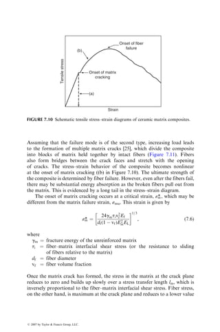
![undergoing large plastic deformations and strain hardening after yielding. In
general, they exhibit higher strain-to-failure and fracture toughness than poly-
mers. Furthermore, since the processing temperature for MMCs is very high,
the difference in thermal contraction between the fibers and the matrix during
cooling can lead to relatively high residual stresses. In some cases, the matrix
may yield under the influence of these residual stresses, which can affect the
stress–strain characteristics as well as the strength of the composite.
7.1.1.1 Continuous-Fiber MMC
Consider an MMC containing unidirectional continuous fibers subjected to a
tensile load in the fiber direction. Assume that the matrix yield strain is lower
than the fiber failure strain. Initially, both fibers and matrix deform elastically.
The longitudinal elastic modulus of the composite is given by the rule of
mixtures:
EL ¼ Efvf þ Emvm: (7:1)
After the matrix reaches its yield strain, it begins to deform plastically, but the
fiber remains elastic. At this point, the stress–strain diagram begins to deviate
from its initial slope (Figure 7.1) and exhibits a new longitudinal modulus,
which is given by:
EL ¼ Efvf þ
ds
d«
m
vm, (7:2)
where
ds
d«
m
is slope of the stress–strain curve of the matrix at the composite
strain «c. The stress–strain diagram of the composite in this region is not elastic.
In addition, it may not be linear if the matrix has a nonuniform strain-
hardening rate.
For brittle fiber MMCs, such as SiC fiber-reinforced aluminum alloys, the
composite strength is limited by fiber fracture, and the MMCs fail as the com-
posite strain becomes equal to the fiber failure strain. For ductile fiber MMCs,
such as tungsten fiber-reinforced copper alloys [5] and beryllium fiber-reinforced
aluminum alloys [6], the fiber also yields and plastically deforms along with the
matrix. In addition, the composite strength is limited by the fiber failure strain,
unless the fibers fail by necking. If the fibers exhibit necking before failure and its
failure strain is lower than that of the matrix, the strain at the ultimate tensile
stress of the composite will be greater than that at the ultimate tensile stress of the
fiber alone.
If the composite failure is controlled by the fiber failure strain, the
longitudinal composite strength is given by
sLtu ¼ sfuvf þ sm
0
(1 vf), (7:3)
ß 2007 by Taylor Francis Group, LLC.](https://image.slidesharecdn.com/fiberreinforcedcompositesmaterialsmanufacturinganddesignp1-220510152925-9ef3de0d/85/Fiber_Reinforced_Composites_Materials_Manufacturing_and_Design_P-1-pdf-559-320.jpg)
![where sm
0
is the matrix flow stress at the ultimate fiber strain that is determined
from the matrix stress–strain diagram.
Equation 7.3 appears to fit the experimental strength values for a number of
MMCs, such as copper matrix composites (Figure 7.2) containing either brittle
or ductile tungsten fibers [5]. In general, they are valid for MMCs in which (1)
there is no adverse interfacial reaction between the fibers and the matrix that
produces a brittle interphase, (2) there is a good bond between the fibers and
the matrix, and (3) the thermal residual stresses at or near the interface are low.
The longitudinal tensile strength predicted by Equation 7.3 is higher than
the experimental values for carbon fiber-reinforced aluminum alloys. In these
systems, unless the carbon fibers are coated with protective surface coating, a
brittle Al4C3 interphase is formed. Cracks initiated in this interphase cause the
fibers to fail at strains that are lower than their ultimate strains. In some cases,
the interfacial reaction is so severe that it weakens the fibers, which fail at very
low strains compared with the unreacted fibers [7]. If the matrix continues to
carry the load, the longitudinal tensile strength of the composite will be
sLtu ¼ smu(1 vf), (7:4)
Brittle
fiber Ductile
fiber
Ductile fiber
composite
Brittle fiber
composite
Secondary modulus
Primary modulus
Matrix
Strain
Stress
FIGURE 7.1 Schematic representation of longitudinal tensile stress–strain diagram of a
unidirectional continuous fiber-reinforced MMC.
ß 2007 by Taylor Francis Group, LLC.](https://image.slidesharecdn.com/fiberreinforcedcompositesmaterialsmanufacturinganddesignp1-220510152925-9ef3de0d/85/Fiber_Reinforced_Composites_Materials_Manufacturing_and_Design_P-1-pdf-560-320.jpg)
![which is less than the matrix tensile strength smu. Thus, in this case, the
matrix is weakened in the presence of fibers instead of getting strengthened
(Figure 7.3).
7.1.1.2 Discontinuously Reinforced MMC
In recent years, the majority of the research effort has been on SiCw- and SiCp-
reinforced aluminum alloys [8]. Titanium, magnesium, and zinc alloys have also
been used; however, they are not discussed in this chapter. Reinforcements
other than SiC, such as Al2O3, have also been investigated. Tensile properties of
some of these composites are given in Appendix A.9.
McDanels [9] has reported the mechanical properties of both SiCw- and
SiCp-reinforced aluminum alloys, such as 6061, 2024=2124, 7075, and 5083.
Reinforcement content is in the range of 10–40 vol%. These composites were
produced by powder metallurgy, followed by extrusion and hot rolling. His
observations are summarized as follows:
1200
1000
800
600
Longitudinal
tensile
strength
(MPa)
400
200
0
0 0.5
Fiber volume fraction, vf
1.0
Equation 7.4
Equation 7.3
FIGURE 7.2 Longitudinal tensile strength variation of a unidirectional continuous
tungsten fiber=copper matrix composite at various fiber volume fractions. (Adapted
from Kelly, A. and Davies, G.J., Metall. Rev., 10, 1, 1965.)
ß 2007 by Taylor Francis Group, LLC.](https://image.slidesharecdn.com/fiberreinforcedcompositesmaterialsmanufacturinganddesignp1-220510152925-9ef3de0d/85/Fiber_Reinforced_Composites_Materials_Manufacturing_and_Design_P-1-pdf-561-320.jpg)
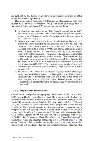
![McDanels [9] did not observe much directionality in SiC-reinforced aluminum
alloys. Since MMCs manufactured by powder metallurgy are transformed into
bars and sheets by hot rolling, it is possible to introduce differences in orien-
tation in SiCw-reinforced alloys with more whiskers oriented in the rolling
direction. Repeated rolling through small roll gaps can break whiskers and
particulates into smaller sizes, thereby reducing the average particle size or the
average length-to-diameter ratio of the whiskers. Both whisker orientation and
size reduction may affect the tensile properties of rolled MMCs.
Johnson and Birt [10] found that the tensile modulus of both SiCp- and
SiCw-reinforced MMCs can be predicted reasonably well using Halpin–Tsai
equations (Equations 3.49 through 3.53). However, the strength and ductility of
MMCs with discontinuous reinforcements are difficult to model in terms of
reinforcement and matrix properties alone, since the matrix microstructure in
the composite may be different from the reinforcement-free matrix due to
complex interaction between the two. The particle size has a significant influ-
ence on yield strength, tensile strength, and ductility of SiCp-reinforced MMCs
[11]. Both yield and tensile strengths increase with decreasing particle size. Such
behavior is attributed to the generation of thermal residual stresses, increase in
dislocation density, and constraints to dislocation motion, all due to the pres-
ence of particles. The ductility of the composite also increases with decreasing
SiCp, 40%
SiCw, 30%
SiCp, 30% SiCp, 20%
SiCw, 20%
SiCw, 10%
SiCp, 15%
SiC/6061 A1 Composites
10
8
6
Strain (percent)
4
2
0
0
100
200
Stress
(MPa)
300
400
500
600
FIGURE 7.4 Tensile stress–strain diagrams of SiCp- and SiCw-reinforced 6061-T6
aluminum alloy composites. (Adapted from McDanels, D.L., Metall. Trans., 16A,
1105, 1985.)
ß 2007 by Taylor Francis Group, LLC.](https://image.slidesharecdn.com/fiberreinforcedcompositesmaterialsmanufacturinganddesignp1-220510152925-9ef3de0d/85/Fiber_Reinforced_Composites_Materials_Manufacturing_and_Design_P-1-pdf-563-320.jpg)
![particle size; however, after attaining a maximum value at particle diameters
between 2 and 4 mm, it decreases rapidly to low values. The failure of the
composite is initiated by cavity formation at the interface or by particle fracture.
Other observations on the thermomechanical properties of SiCp- or SiCw-
reinforced aluminum alloys are
1. Both CTE and thermal conductivity of aluminum alloys are reduced by
the addition of SiCp [11,12].
2. The fracture toughness of aluminum alloys is reduced by the addition of
SiCp. Investigation by Hunt and his coworkers [13] indicates that frac-
ture toughness is also related to the particle size. They have also
observed that overaging, a heat treatment process commonly used for
7000-series aluminum alloys to enhance their fracture toughness, may
produce lower fracture toughness in particle-reinforced aluminum
alloys.
3. The long-life fatigue strength of SiCw-reinforced aluminum alloys is
higher than that of the unreinforced matrix, whereas that of SiCp-
reinforced aluminum alloys is at least equal to that of the unreinforced
matrix (Figure 7.5).
4. The high-temperature yield strength and ultimate tensile strength of
SiC-reinforced aluminum alloys are higher than the corresponding
values of unreinforced alloys. The composite strength values follow
similar functional dependence on temperature as the matrix strength
values (Figure 7.6).
42
35
Alternating
stress
(MPa)
28
21
14
7
0
103
104
105
106
Cycles to failure
SiCw/6061–Al
6061 Al Matrix
SiCp/6061–Al
107
108
FIGURE 7.5 S–N curves for SiCw- and SiCp-reinforced 6061 aluminum alloy. (Adapted
from Rack, H.J. and Ratnaparkhi, P., J. Metals, 40, 55, 1988.)
ß 2007 by Taylor Francis Group, LLC.](https://image.slidesharecdn.com/fiberreinforcedcompositesmaterialsmanufacturinganddesignp1-220510152925-9ef3de0d/85/Fiber_Reinforced_Composites_Materials_Manufacturing_and_Design_P-1-pdf-564-320.jpg)
![5. Karayaka and Sehitoglu [14] conducted strain-controlled fatigue tests
on 20 vol% SiCp-reinforced 2xxx-T4 aluminum alloys at 2008C and
3008C. Based on stress range, the reinforced alloys have a superior
fatigue performance than the unreinforced alloys.
6. Creep resistance of aluminum alloys is improved by the addition of
either SiCw or SiCp. For example, Morimoto et al. [15] have shown
that the second-stage creep rate of 15 vol% SiCw-reinforced 6061 alu-
minum alloy is nearly two orders of magnitude lower than that of the
unreinforced alloy (Figure 7.7).
2024 Al
2024 Al
21 vol% SiC/2024 Al
21 vol% SiC/2024 Al
500
400
Ultimate
tensile
strength,
MPa
Yield
strength,
MPa
300
200
100
0
400
300
200
100
0
0 100 200
Temperature, ⬚C
300 400 0 100 200
Temperature, ⬚C
300 400
FIGURE 7.6 Effects of increasing temperature on the ultimate tensile strength and yield
strength of unreinforced and 21 vol% SiC-reinforced 2024 aluminum alloy. (Adapted
from Nair, S.V., Tien, J.K., and Bates, R.C., Int. Metals Rev., 30, 275, 1985.)
0
0
1
Strain,
%
2
0.5
Time, 105 s
1.0 1.5
6061 Al
s =26 MPa
15 vol% SiCw/6061
s =70 MPa
T =300°C
FIGURE 7.7 Comparison of creep strains of unreinforced and 15 vol% SiCw-reinforced
6061 aluminum alloy. (Adapted from Morimoto, T., Yamaoka, T., Lilholt, H., and
Taya, M., J. Eng. Mater. Technol., 110, 70, 1988.)
ß 2007 by Taylor Francis Group, LLC.](https://image.slidesharecdn.com/fiberreinforcedcompositesmaterialsmanufacturinganddesignp1-220510152925-9ef3de0d/85/Fiber_Reinforced_Composites_Materials_Manufacturing_and_Design_P-1-pdf-565-320.jpg)
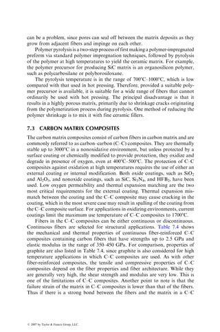
![is raised and held for a length of time to complete the consolidation of layers
into the final thickness. Typically, the temperature is 50%–90% of the solidus
temperature of the matrix, and the pressure ranges from 10 to 120 MPa (1.45–
17.4 ksi). Afterward, the cooling is carried out at a controlled rate and under
pressure to reduce residual stresses as well as to prevent warping.
The consolidation of layers in VHP takes place through diffusion bonding,
plastic deformation, and creep of the metal matrix [16]. The basic process param-
eters that control the quality of consolidation are temperature, pressure, and
holding time. Another important parameter is the cleanliness of the layers to be
joined. Polymeric binder residues or oxide scales can cause poor bonding between
the fibers and the matrix as well as between the matrices in various layers. There-
fore, careful surface preparation before stacking the layers can be very beneficial.
7.1.2.2 Discontinuously Reinforced MMC
7.1.2.2.1 Powder Metallurgy
In this process, atomized metal powders (typically with a mean diameter of
15 mm or 325 mesh size) are blended with deagglomerated whiskers
or particulates. Deagglomeration may involve agitation of a liquid suspension
of the reinforcement in an ultrasonic bath. The blended mixture is cold-
compacted in a graphite die, outgassed, and vacuum hot-pressed to form a
cylindrical billet. The pressure is applied in the hot-pressing stage only after the
temperature is raised above the solidus temperature of the matrix alloy.
Currently available SiCp-reinforced aluminum billets range from 15 cm
(6 in.) to 44.5 cm (17.5 in.) in diameter. Most billets are extruded to rods or
rectangular bars using lubricated conical or streamline dies. Various structural
shapes can be fabricated from these rods and bars using hot extrusion, while
sheets and plates can be produced by hot rolling on conventional rolling mills.
Other metalworking processes, such as forging and shear spinning, can also be
used for shaping them into many other useable forms.
Typical tensile properties of SiCw- and SiCp-reinforced aluminum alloys are
given in Table 7.2. All of these composites were manufactured by powder
metallurgy and then extruded to rods or bars. Sheets were formed by hot rolling
the bars. Following observations can be made from the table:
1. The secondary processing of extrusion and rolling can create significant
difference in tensile properties in the longitudinal and transverse direc-
tions, especially in whisker-reinforced composites.
2. Ultimate tensile strength, yield strength, and modulus of discontinuously
reinforced aluminum alloys increase with increasing reinforcement
content, but elongation to failure (which is related to ductility) decreases.
3. For the same reinforcement content, whiskers produce stronger and
stiffer composites than particulates.
ß 2007 by Taylor Francis Group, LLC.](https://image.slidesharecdn.com/fiberreinforcedcompositesmaterialsmanufacturinganddesignp1-220510152925-9ef3de0d/85/Fiber_Reinforced_Composites_Materials_Manufacturing_and_Design_P-1-pdf-567-320.jpg)
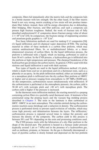
![fiber surface. The viscosity of molten aluminum or other alloys is very low
(almost two orders of magnitude lower than that of liquid epoxy and five to
seven orders of magnitude lower than that of liquid thermoplastics). However,
there is, in general, poor wettability between the fibers and the liquid metal,
which may affect the infiltration process. The wettability is improved by
increasing fiber=atmosphere surface tension or by reducing the liquid
metal=fiber surface tension [17]. Both approaches reduce the fiber wetting
angle (Figure 7.9) and, therefore, improve wetting between the fibers and the
matrix. Common methods of improving wettability are
1. Control the chemical environment in which the infiltration is conducted.
For example, controlling the oxygen content of the environment can
improve the wettability of aluminum alloys with carbon fibers. This
is because aluminum has a strong affinity toward atmospheric oxygen.
As the hot liquid metal comes in contact with air, a thin, adherent
aluminum oxide layer is formed on its surface, which interferes with
wetting.
2. Add an alloying element that modifies or disrupts the surface oxide
layer. For example, magnesium added to aluminum alloys disrupts the
surface oxide and improves wettability with most reinforcements.
3. Use a coating on the reinforcement surface that promotes wetting.
Suitable coatings may also prevent unwanted chemical reaction between
the fibers and the matrix. For example, aluminum reacts with carbon
fibers above 5508C to form Al4C3 platelets, which cause pitting on the
carbon fiber surface and reduce the fiber tensile strength.
In general, for high cooling rates and low reinforcement levels (i.e., large
interfiber spacings), the matrix microstructure in the solidified MMC is similar
to that observed in a reinforcement-free alloy. However, for slower cooling
V
S
gLV
gSL gSV
L q
V
S
gLV
gSL gSV
L q
V=Vapor (atmosphere), L=Liquid metal, S=Solid (fiber)
For good wettability, gSV − gSL gLV cosq
(a) Good wetting (b) Poor wetting
FIGURE 7.9 Surface energy requirement for good fiber surface wetting.
ß 2007 by Taylor Francis Group, LLC.](https://image.slidesharecdn.com/fiberreinforcedcompositesmaterialsmanufacturinganddesignp1-220510152925-9ef3de0d/85/Fiber_Reinforced_Composites_Materials_Manufacturing_and_Design_P-1-pdf-569-320.jpg)
![rates or high reinforcement levels, the matrix microstructure in the MMC can
be significantly different from that of the reinforcement-free alloy [18,19]. Some
of the observed microstructural differences are
1. Matrix microsegregation may be reduced.
2. The crystal morphology may change from cellular dendritic to com-
pletely featureless.
3. Certain primary phases may nucleate preferentially at the reinforcement
surface (e.g., silicon in a hypereutectic Al–Si alloy nucleating on the
surfaces of carbon fibers or SiC particles).
4. If the reinforcement is relatively mobile, it can be pushed by growing
dendrites into the last freezing zone, thereby creating an uneven distri-
bution of the reinforcement in the composite.
5. If the fibers are held below the liquidus temperature of the matrix alloy,
the liquid melt is very rapidly cooled as it comes in contact with the
fibers and solidification begins at the fiber surface. This leads to finer
grain size, which is of the order of the fiber diameter.
7.1.2.2.3 Compocasting
When a liquid metal is vigorously stirred during solidification by slow cooling,
it forms a slurry of fine spheroidal solids floating in the liquid. Stirring at high
speeds creates a high shear rate, which tends to reduce the viscosity of the slurry
even at solid fractions that are as high as 50%–60% by volume. The process of
casting such a slurry is called rheocasting. The slurry can also be mixed with
particulates, whiskers, or short fibers before casting. This modified form of
rheocasting to produce near net-shape MMC parts is called compocasting.
The melt-reinforcement slurry can be cast by gravity casting, die-casting,
centrifugal casting, or squeeze casting. The reinforcements have a tendency to
either float to the top or segregate near the bottom of the melt due to the
differences in their density from that of the melt. Therefore, a careful choice of
the casting technique as well as the mold configuration is of great importance in
obtaining uniform distribution of reinforcements in a compocast MMC [20].
Compocasting allows a uniform distribution of reinforcement in the matrix
as well as a good wet-out between the reinforcement and the matrix. Continuous
stirring of the slurry creates an intimate contact between them. Good bonding
is achieved by reducing the slurry viscosity as well as increasing the mixing time.
The slurry viscosity is reduced by increasing the shear rate as well as increasing
the slurry temperature. Increasing mixing time provides longer interaction
between the reinforcement and the matrix.
7.1.2.2.4 Squeeze Casting
Squeeze casting is a net-shape metal casting process and involves solidification
of liquid metal under pressure. It differs from the more familiar process of
ß 2007 by Taylor Francis Group, LLC.](https://image.slidesharecdn.com/fiberreinforcedcompositesmaterialsmanufacturinganddesignp1-220510152925-9ef3de0d/85/Fiber_Reinforced_Composites_Materials_Manufacturing_and_Design_P-1-pdf-570-320.jpg)
![pressure die-casting in which pressure is used only to inject the liquid metal into
a die cavity and the solidification takes place under little or no pressure. In
squeeze casting, high pressure is maintained throughout solidification. This
leads to a fine equiaxed grain structure and very little porosity in the cast
component. In general, squeeze-cast metals have higher tensile strengths as
well as greater strains-to-failure than the gravity-cast or die-cast metals. In
addition, since the use of pressure increases castability, a wide variety of alloy
compositions can be squeeze cast, including the wrought alloys that are usually
considered unsuitable for casting because of their poor fluidity.
Squeeze casting, as it applies to MMC, starts by placing a preheated fiber
preform in an open die cavity, which is mounted in the bottom platen of a
hydraulic press. A measured quantity of liquid metal is poured over the
preform, the die cavity is closed, and pressure up to 100 MPa is applied to
force the liquid metal into the preform. The pressure is released only after the
solidification is complete.
Squeeze casting has been used to produce a variety of MMCs, including
those with wrought aluminum alloys, such as 2024, 6061, and 7075. However,
several investigators [21,22] have suggested that improved properties are
obtained by alloy modification of commercial alloys. Other variables that
may influence the quality of a squeeze-cast MMC are the temperatures of the
molten metal as well as the fiber preform, infiltration speed, and the final
squeeze pressure [22,23].
7.2 CERAMIC MATRIX COMPOSITES
Structural ceramics such as silicon carbide (SiC), silicon nitride (Si3N4), and
aluminum oxide (Al2O3) are considered candidate materials for applications in
internal combustion engines, gas turbines, electronics, and surgical implants.
They are high-modulus materials with high temperature resistance (Table 7.3);
however, they have low failure strains and very low fracture toughness. Poor
structural reliability resulting from their brittleness and high notch sensitivity is
the principal drawback for widespread applications of these materials.
The impetus for developing ceramic matrix composites comes from the
possibility of improving the fracture toughness and reducing the notch sensi-
tivity of structural ceramics [24]. Early work on ceramic matrix composites used
carbon fibers in reinforcing low- to intermediate-modulus ceramics, such as
glass and glass-ceramics. Recent work on ceramic matrix composites has
focused on incorporating SiC fibers or whiskers into high-temperature-resistant
polycrystalline ceramics, such as SiC and Si3N4. Since the modulus values of
these materials are close to those of fibers, there is very little reinforcement
effect from the fibers. Instead, the heterogeneous nature of the composite
contributes to the increase in matrix toughness through several microfailure
mechanisms as described in the following section.
ß 2007 by Taylor Francis Group, LLC.](https://image.slidesharecdn.com/fiberreinforcedcompositesmaterialsmanufacturinganddesignp1-220510152925-9ef3de0d/85/Fiber_Reinforced_Composites_Materials_Manufacturing_and_Design_P-1-pdf-571-320.jpg)
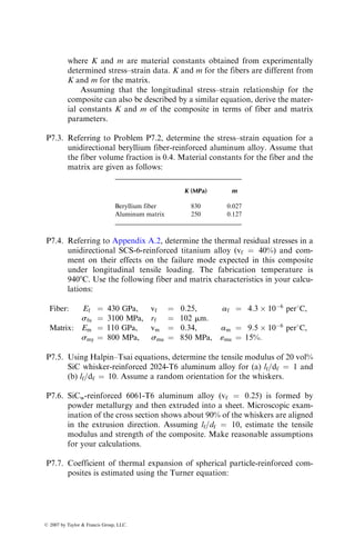
![Assuming that the failure mode is of the second type, increasing load leads
to the formation of multiple matrix cracks [25], which divide the composite
into blocks of matrix held together by intact fibers (Figure 7.11). Fibers
also form bridges between the crack faces and stretch with the opening
of cracks. The stress–strain behavior of the composite becomes nonlinear
at the onset of matrix cracking ((b) in Figure 7.10). The ultimate strength of
the composite is determined by fiber failure. However, even after the fibers fail,
there may be substantial energy absorption as the broken fibers pull out from
the matrix. This is evidenced by a long tail in the stress–strain diagram.
The onset of matrix cracking occurs at a critical strain, «m
* , which may be
different from the matrix failure strain, «mu. This strain is given by
«m
* ¼
24gmtiv2
f Ef
df(1 vf)E2
mEL
1=3
, (7:6)
where
gm ¼ fracture energy of the unreinforced matrix
ti ¼ fiber–matrix interfacial shear stress (or the resistance to sliding
of fibers relative to the matrix)
df ¼ fiber diameter
vf ¼ fiber volume fraction
Once the matrix crack has formed, the stress in the matrix at the crack plane
reduces to zero and builds up slowly over a stress transfer length lm, which is
inversely proportional to the fiber–matrix interfacial shear stress. Fiber stress,
on the other hand, is maximum at the crack plane and reduces to a lower value
Onset of fiber
failure
(b)
(a)
Onset of matrix
cracking
Strain
Tensile
stress
FIGURE 7.10 Schematic tensile stress–strain diagrams of ceramic matrix composites.
ß 2007 by Taylor Francis Group, LLC.](https://image.slidesharecdn.com/fiberreinforcedcompositesmaterialsmanufacturinganddesignp1-220510152925-9ef3de0d/85/Fiber_Reinforced_Composites_Materials_Manufacturing_and_Design_P-1-pdf-573-320.jpg)
![Evans and Marshall [26] have made the following suggestions for promoting
debonding and fiber pull-out:
1. The fracture energy required for debonding, Gic, should be sufficiently
small compared with that for fiber fracture, Gfc:
Gic
Gfc
1
4
:
2. Residual radial strain at the interface due to matrix cooling from the
processing temperature should be tensile instead of compressive.
3. Sliding resistance between the fibers and the matrix should be small,
which means the friction coefficient along the debonded interface should
also be small (~0.1).
4. Long pull-out lengths are expected with fibers having a large variability
in their strength distribution; however, for high composite strength, the
median value of the fiber strength distribution should be high.
As suggested in the preceding discussion and also verified experimentally, the
fracture toughness of a ceramic matrix composite is improved if there is poor
bonding between the fibers and the matrix. This can be achieved by means of a
fiber coating or by segregation at the fiber–matrix interface. The most common
method is to use a dual coating in which the inner coating meets the require-
ments for debonding and sliding, and the outer coating protects the fiber
surface from degradation at high processing temperatures.
7.2.2 MECHANICAL PROPERTIES
7.2.2.1 Glass Matrix Composites
Development of ceramic matrix composites began in the early 1970s with
carbon fiber-reinforced glass and glass-ceramic composites. Research by
Sambell et al. [27,28] on carbon fiber-reinforced borosilicate (Pyrex) glass
showed the following results:
1. Increasing fiber volume fraction increases both flexural strength and
flexural modulus of the composite containing continuous fibers.
2. The fracture energy of the glass matrix, as measured by the area under
the load–deflection diagrams of notched flexural specimens, increases
significantly by the addition of continuous carbon fibers. For example,
the fracture energy of 40 vol% carbon fiber-borosilicate glass is 3000
J=m2
compared with only 3 J=m2
for borosilicate glass. The flexural
strength for the same composite is 680 MPa compared with 100 MPa for
the matrix alone. The load–deflection diagram for the matrix is linear up
ß 2007 by Taylor Francis Group, LLC.](https://image.slidesharecdn.com/fiberreinforcedcompositesmaterialsmanufacturinganddesignp1-220510152925-9ef3de0d/85/Fiber_Reinforced_Composites_Materials_Manufacturing_and_Design_P-1-pdf-575-320.jpg)
![to failure, whereas that for the composite is linear up to 340 MPa. The
load–deflection diagram becomes nonlinear at this stress due to matrix
cracking on the tension side of the flexural specimen.
3. Random fiber orientation of short carbon fibers produces flexural
strengths that are lower than that of borosilicates; however, the fracture
energy (work of fracture) increases with fiber volume fraction, as shown
in Figure 7.12.
Prewo and Brennan [29] have reported that carbon fiber-reinforced borosilicate
glass retains its flexural strength up to 6008C. Above this temperature, the
composite strength is reduced due to matrix softening. Thus, although glass
matrix is attractive for its lower processing temperature, its application tempera-
ture is limited to 6008C. An alternative is to replace glass with a glass-ceramic,
such as lithium aluminosilicate (LAS), which increases the use temperature to
10008C or higher. Since carbon fibers are prone to oxidation above 3008C, they
400
1: Carbon fibers (aligned)
in borosilicate glass
2: Carbon fibers (random)
in borosilicate glass
3: Carbon fibers
in Mg0
4: Carbon fibers
in glass-ceramic
1
2
3
4
300
200
100
0
0 10 20 30
Fiber volume fraction
Work
of
fracture
(J/m
2
)
40
FIGURE 7.12 Work of fracture of various glass matrix composites. (Adapted from
Sambell, R.A.J., Bowen, D.H., and Phillips, D.C., J. Mater. Sci., 7, 663, 1972.)
ß 2007 by Taylor Francis Group, LLC.](https://image.slidesharecdn.com/fiberreinforcedcompositesmaterialsmanufacturinganddesignp1-220510152925-9ef3de0d/85/Fiber_Reinforced_Composites_Materials_Manufacturing_and_Design_P-1-pdf-576-320.jpg)
![are replaced by SiC fibers, which show no appreciable reduction in either
strength or modulus up to 8008C.
Thermomechanical properties of SiC-reinforced glass-ceramics have been
studied by a number of investigators [30,31]. The results of investigations on
Nicalon (SiC) fiber-reinforced LAS are summarized as follows:
1. Nicalon=LAS composites retain their flexural strength up to 8008C
when tested in air, and up to 11008C when tested in an inert atmosphere,
such as argon. The fracture mode of these composites depends strongly
on the test environment.
2. Room-temperature tension test in air of unidirectional Nicalon=LAC
composites shows multiple matrix cracking and fiber pull-out. The
composite fails gradually after the maximum load is reached. When
the same composite is tested at 9008C and above, fiber failure occurs
after one single matrix crack has formed, resulting in a catastrophic
failure with sudden load drop. This change in failure mode is attributed
to fiber strength degradation as well as increased fiber–matrix bonding
in the oxidative atmosphere. The initial carbon-rich layer between the
SiC fiber and the LAS matrix is replaced by an amorphous silicate due
to oxidation at 6508C–10008C. This creates a strong interfacial bond and
transforms the composite from a relatively tough material to a brittle
material [31].
3. The presence of a carbon-rich interface is very important in obtaining a
strong, tough SiC fiber-reinforced LAS composite, since this interface is
strong enough to transfer the load from the matrix to the fibers, yet
weak enough to debond before fiber failure. This enables the composite
to accumulate a significant amount of local damage without failing in a
brittle mode.
7.2.2.2 Polycrystalline Ceramic Matrix
Ceramic matrix composites using polycrystalline ceramic matrix, such as SiC,
Si3N4, and ZrO2–TiO2, are also developed. These matrices offer higher tem-
perature capabilities than glasses or glass-ceramics. Research done by Rice and
Lewis [32] on unidirectional Nicalon (SiC) fiber-reinforced ZrO2–TiO2 and
ZrO2–SiO2 composites shows the importance of proper fiber–matrix bonding
in achieving high flexural strength and fracture toughness in ceramic matrix
composites. The BN coating used on Nicalon fibers in their work creates a
weaker bond than if the fibers are uncoated. The composite with coated fibers
has a flexural strength of 400–900 MPa (60–125 ksi), compared with 70–220
MPa (10–32 ksi) for uncoated fibers. The difference in flexural load–deflection
diagrams of coated and uncoated fiber composites is shown in Figure 7.13. The
coated fibers not only increased the strength but also created a noncatastrophic
failure mode with significant fiber pull-out. Fracture toughness of coated fiber
ß 2007 by Taylor Francis Group, LLC.](https://image.slidesharecdn.com/fiberreinforcedcompositesmaterialsmanufacturinganddesignp1-220510152925-9ef3de0d/85/Fiber_Reinforced_Composites_Materials_Manufacturing_and_Design_P-1-pdf-577-320.jpg)
![composites is 20 MPa m1=2
, compared with about 1 MPa m1=2
for uncoated
fiber composites.
Thomson and LeCostaonec [33] reported the tensile and flexural properties
of Si3N4 matrix reinforced with unidirectional and bidirectional SiC monofila-
ments. The fibers are designated as SCS-6 (filament diameter ¼ 140 mm) and
SCS-9 (filament diameter ¼ 75 mm), both having a double carbon-rich layer on
the outside surface. The purpose of the double layer is to enhance the fiber
strength as well as to promote debonding. As demonstrated in Figure 7.14,
SCS-reinforced Si3N4 composites exhibit considerable load-carrying capability
and toughness beyond the initial matrix microcracking at both 238C and 13508C.
7.2.3 MANUFACTURING PROCESSES
The manufacturing processes for ceramic matrix composites can be divided into
two groups.
7.2.3.1 Powder Consolidation Process
This is a two-step process of first making a ‘‘green’’ compact, followed by
hot pressing the compact into the final shape (Figure 7.15). Hot pressing at
Max. stress=280 MPa (40 ksi)
Coated SiC fibers
in SiO2 matrix
Max. stress =
80 MPa (11 ksi)
Uncoated SiC fibers
in SiO2 matrix
Deflection
Load
FIGURE 7.13 Effect of fiber surface coating on the room temperature flexural load-
deflection diagrams of SiC (Nicalon)-reinforced SiO2. (Adapted from Rice, R.W. and
Lewis, D., III, Reference Book for Composites Technology, Vol. 1, S.M. Lee, ed.,
Technomic Pub. Co., Lancaster, PA, 1989.)
ß 2007 by Taylor Francis Group, LLC.](https://image.slidesharecdn.com/fiberreinforcedcompositesmaterialsmanufacturinganddesignp1-220510152925-9ef3de0d/85/Fiber_Reinforced_Composites_Materials_Manufacturing_and_Design_P-1-pdf-578-320.jpg)
![temperatures ranging from 12008C to 16008C is used to consolidate the com-
pact into a dense material with as little porosity as possible.
There are various ways of making the green compact. For continuous
fibers, the compact is made by stacking a number of tapes, which are cut
from a sheet of fiber yarns infiltrated with the matrix. The sheet is produced
by pulling a row of parallel fiber yarns through a tank containing a colloidal
slurry of the matrix and winding it around a drum. The compact can also be
made by infiltrating a fiber preform with either a matrix slurry or a colloidal sol
prepared from alkoxides and other organic precursors.
The green compact is consolidated and transformed into a dense compos-
ite either by VHP in a press or by hot isotactic pressing (HIP) inside an
autoclave. VHP is commonly used; however, it is limited to producing only
simple shapes, such as plates, rods, or blocks. To reduce porosity in the
composite, the hot-pressing temperature is selected in the range of 1008C–
2008C higher than that for hot pressing the matrix alone. In some cases, such
high temperatures may cause fiber degradation as well as undesirable reactions
at the fiber–matrix interface. Rice and Lewis [32] have shown that the strength
and toughness of hot-pressed ceramic matrix composites depend strongly on
the processing conditions, which include temperature, pressure, and time.
Fiber degradation and adverse fiber–matrix reactions can be reduced with a
fiber coating as well as by using an inert atmosphere (such as argon) during
hot pressing.
The processing temperature is usually lower in HIP. Since pressure is
applied equally in all directions instead of uniaxially as in VHP, it is also
capable of producing more intricate net-shape structures with higher density
and greater uniformity. However, in HIP, the compact must be enclosed in a
gas-permeable envelope (called the ‘‘can’’) which is removed after processing.
Finding a suitable canning material frequently poses a problem.
7.2.3.2 Chemical Processes
Two common chemical processes are chemical vapor infiltration (CVI) and
polymer pyrolysis. They are briefly described as follows.
In CVI, the ceramic matrix is deposited on fibers from a gaseous medium by
passing it over a preheated fiber preform in a controlled environment. The gas
is selected such that it either reacts or decomposes when it comes in contact
with the fibers. The temperature range for CVI is 10008C–12008C, which is
lower than the hot-pressing temperature. For example, SiC matrix can be
deposited on SiC fibers by passing methyltrichlorosilane over the SiC fiber
preform in the presence of hydrogen at 12008C [34].
The advantages of CVI are that (1) it can be used to produce a variety of
shapes, (2) there is a uniform distribution of matrix in the composite, and
(3) fibers undergo less mechanical damage, although the possibility of chemical
degradation due to contact with the gas exists. Controlling the porosity in CVI
ß 2007 by Taylor Francis Group, LLC.](https://image.slidesharecdn.com/fiberreinforcedcompositesmaterialsmanufacturinganddesignp1-220510152925-9ef3de0d/85/Fiber_Reinforced_Composites_Materials_Manufacturing_and_Design_P-1-pdf-580-320.jpg)
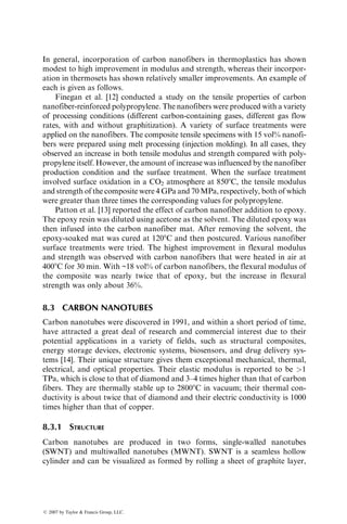
![composite, fibers fail immediately after the matrix fails and the composite fails
in a brittle manner with low strength. On the other hand, if the fiber–matrix
bond is not very strong, matrix cracking at low strain will not produce imme-
diate fiber failure; instead, there will be energy absorption due to debonding,
fiber bridging, fiber fracture, and fiber pull-out, and such a composite can
possess high fracture toughness. Indeed, the work of fracture test of fully
densified unidirectional C–C composites shows fracture energy value of about
2 3 104
J=m2
[35]. In comparison, the fracture energy of engineering ceramics
and premium-grade graphite is 102
J=m2
.
Two basic fabrication methods are used for making C–C composites [36]:
(1) liquid infiltration and (2) chemical vapor deposition (CVD). The starting
material in either of these methods is a carbon fiber preform, which may
contain unidirectional fibers, bi- or multidirectional fabrics, or a three-
dimensional structure of carbon fibers. In the liquid infiltration process, the
preform is infiltrated with a liquid, which on heating, carbonizes to yield at
least 50 wt% carbon. In the CVD process, a hydrocarbon gas is infiltrated into
the preform at high temperature and pressure. The chemical breakdown of the
hydrocarbon gas produces the carbon matrix. In general, CVD is used with thin
sections and liquid infiltration is used with thick sections.
Two types of liquids are used in the liquid infiltration method: (1) pitch,
which is made from coal tar or petroleum and (2) a thermoset resin, such as a
phenolic or an epoxy. In the pitch infiltration method, either an isotropic pitch
or a mesophase pitch is infiltrated into the dry carbon fiber preform at 10008C
or higher and at pressure ranging from atmospheric to 207 MPa (30,000 psi).
At this temperature, carbonization occurs simultaneously with infiltration. If
the carbonization is performed at the atmospheric pressure, the carbon yield is
50–60 wt% with isotropic pitch and 80 wt% with mesophase pitch. The
carbon yield is higher if the pressure is increased.
In the thermoset resin infiltration method, the starting material is a prepreg
containing carbon fibers in a partially cured thermoset resin. A laminate is first
constructed using the prepreg layers and the vacuum bag molding process
described in Chapter 5. The resin in the laminate is then carbonized at
8008C–10008C in an inert atmosphere. The volatiles emitted during the carbon-
ization reaction cause shrinkage and a reduction in density. The carbonization
process is performed slowly to prevent rapid evolution of volatiles, which may
cause high porosity and delamination between the layers. The infiltration=
carbonization process is repeated several times to reduce the porosity and
increase the density of the composite. The carbon yield in this process is
between 50% and 70% depending on the resin and processing conditions used.
The CVD process starts with the fabrication of a dry fiber preform in the
shape of the desired part. The preform is heated in a furnace under pressure
(typically around 1 psi or 7 kPa) and in the presence of a hydrocarbon gas,
such as methane, propane, or benzene. As the gas is thermally decomposed, a
layer of pyrolitic carbon is slowly formed and deposited on the hot preform
ß 2007 by Taylor Francis Group, LLC.](https://image.slidesharecdn.com/fiberreinforcedcompositesmaterialsmanufacturinganddesignp1-220510152925-9ef3de0d/85/Fiber_Reinforced_Composites_Materials_Manufacturing_and_Design_P-1-pdf-583-320.jpg)
![surface. In the isothermal CVD process, the temperature of the furnace is
maintained constant at 11008C. Since the pyrolitic carbon deposited on the
surface tends to close the pores located at and very close to the surface, it
becomes difficult to fill the internal pores with carbon. Thus it may be
necessary to lightly machine the preform surfaces to remove the surface carbon
layer and then repeat the infiltration process. The infiltration is better if either
a thermal gradient or a pressure gradient is created across the thickness of the
preform. In the thermal gradient technique, one surface is maintained at a
higher temperature than the other, and the carbon infiltration progresses from
the hotter surface to the colder surface. In the pressure gradient technique, a
pressure differential is created across the thickness, which forces the hydro-
carbon gas to flow through the pores in the preform and deposit carbon
throughout the thickness. With both these techniques, very little, if any,
crust is formed on the surfaces.
The C–C composite obtained by either liquid infiltration or by CVD can be
heated further to transform the carbon matrix from amorphous form to gra-
phitic form. The graphitization temperature is between 21008C and 30008C.
Graphitization increases both strength and modulus of the C–C composite,
while the fracture toughness depends on the graphitization temperature. For
example, for a pitch-based matrix, the optimum graphitization temperature is
27008C, above which fracture toughness starts to decrease [37].
Depending on the starting material and the process condition, the micro-
structure of carbon matrix in C–C composites may vary from small, randomly
oriented crystallites of turbostratic carbon to large, highly oriented, and graph-
itized crystallites. The carbon matrix may also contain large amount of poros-
ity, which causes the density to be lower than the maximum achievable density
of approximately 1.8–2 g=cm3
. There may also be microcracks originating from
thermal stresses as the C–C composite cools down from the processing tem-
perature to room temperature. Since porosity affects not only the density, but
also the properties of the composite, repeated impregnation and carbonization
cycles are used to reduce the porosity. This process is often referred to as
densification.
REFERENCES
1. R.K. Everett and R.J. Arsenault (eds.), Metal Matrix Composites: Mechanisms and
Properties, Academic Press, San Diego (1991).
2. R.K. Everett and R.J. Arsenault (eds.), Metal Matrix Composites: Processing and
Interfaces, Academic Press, San Diego (1991).
3. T.W. Clyne and P.J. Withers, An Introduction to Metal Matrix Composites, Cam-
bridge University Press, Cambridge, UK (1993).
4. N. Chawla and K.K. Chawla, Metal Matrix Composites, Springer, New York (2006).
5. A. Kelly and G.J. Davies, The principles of the fibre reinforcement of metals,
Metall. Rev., 10:1 (1965).
ß 2007 by Taylor Francis Group, LLC.](https://image.slidesharecdn.com/fiberreinforcedcompositesmaterialsmanufacturinganddesignp1-220510152925-9ef3de0d/85/Fiber_Reinforced_Composites_Materials_Manufacturing_and_Design_P-1-pdf-584-320.jpg)
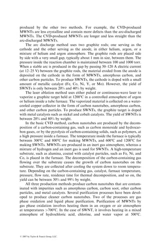
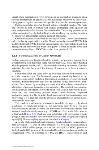
![ac ¼
vrKrar þ vmKmam
vrKr þ vmKm
,
where
K ¼ Bulk modulus ¼
E
3(1 2n)
v ¼ volume fraction
a ¼ CTE
E ¼ modulus
n ¼ Poisson’s ratio
Subscripts r and m represent reinforcement and matrix, respectively
Using the Turner equation and assuming SiC particulates to be spher-
ical, plot the coefficient of thermal expansion of SiCP-reinforced 6061
aluminum alloy as a function of reinforcement volume fraction. Assume
ar ¼ 3.8 3 106
per 8C, Er ¼ 450 GPa, nr ¼ 0.17.
For comparison, experimental values of ac are reported as 16.25 3
106
and 10.3 3 106
per 8C at vr ¼ 25% and 50%, respectively.
P7.8. The steady-state (secondary) creep rate of both unreinforced and
reinforced metallic alloys has been modeled by the following power-
law equation:
_
« ¼ Asn
exp
E
RT
,
where
_
« ¼ steady-state creep rate (per s)
A ¼ constant
s ¼ stress (MPa)
n ¼ stress exponent
E ¼ activation energy
R ¼ universal gas constant
T ¼ temperature (8K)
1. Plot the following constant temperature creep data (Ref. [15])
obtained at 3008C on an appropriate graph and determine the values
of A and n. Assume the activation energies for 6061 aluminum alloy
and SiCw=6061 as 140 and 77 kJ=mol, respectively.
2. Compare the creep rates of the above two materials at 70 MPa and
2508C.
ß 2007 by Taylor Francis Group, LLC.](https://image.slidesharecdn.com/fiberreinforcedcompositesmaterialsmanufacturinganddesignp1-220510152925-9ef3de0d/85/Fiber_Reinforced_Composites_Materials_Manufacturing_and_Design_P-1-pdf-588-320.jpg)
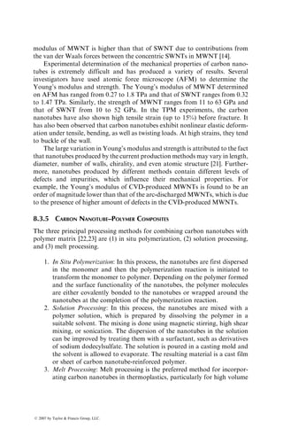
![8 Polymer Nanocomposites
Polymer nanocomposites are polymer matrix composites in which the
reinforcement has at least one of its dimensions in the nanometer range
(1 nanometer (nm) ¼ 103
mm (micron) ¼ 109
m). These composites show
great promise not only in terms of superior mechanical properties, but also in
terms of superior thermal, electrical, optical, and other properties, and, in
general, at relatively low-reinforcement volume fractions. The principal reasons
for such highly improved properties are (1) the properties of nano-reinforce-
ments are considerably higher than the reinforcing fibers in use and (2) the ratio
of their surface area to volume is very high, which provides a greater interfacial
interaction with the matrix.
In this chapter, we discuss three types of nanoreinforcements, namely
nanoclay, carbon nanofibers, and carbon nanotubes. The emphasis here will
be on the improvement in the mechanical properties of the polymer matrix. The
improvement in other properties is not discussed in this chapter and can be
found in the references listed at the end of this chapter.
8.1 NANOCLAY
The reinforcement used in nanoclay composites is a layered silicate clay min-
eral, such as smectite clay, that belongs to a family of silicates known as 2:1
phyllosilicates [1]. In the natural form, the layered smectite clay particles are
6–10 mm thick and contain 3000 planar layers. Unlike the common clay
minerals, such as talc and mica, smectite clay can be exfoliated or delaminated
and dispersed as individual layers, each ~1 nm thick. In the exfoliated form, the
surface area of each nanoclay particle is ~750 m2
=g and the aspect ratio is 50.
The crystal structure of each layer of smectite clays contains two outer
tetrahedral sheets, filled mainly with Si, and a central octahedral sheet of
alumina or magnesia (Figure 8.1). The thickness of each layer is ~1 nm, but
the lateral dimensions of these layers may range from 200 to 2000 nm. The
layers are separated by a very small gap, called the interlayer or the gallery. The
negative charge, generated by isomorphic substitution of Al3þ
with Mg2þ
or
Mg2þ
with Liþ
within the layers, is counterbalanced by the presence of
hydrated alkaline cations, such as Na or Ca, in the interlayer. Since the forces
that hold the layers together are relatively weak, it is possible to intercalate
small organic molecules between the layers.
ß 2007 by Taylor Francis Group, LLC.](https://image.slidesharecdn.com/fiberreinforcedcompositesmaterialsmanufacturinganddesignp1-220510152925-9ef3de0d/85/Fiber_Reinforced_Composites_Materials_Manufacturing_and_Design_P-1-pdf-590-320.jpg)
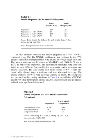
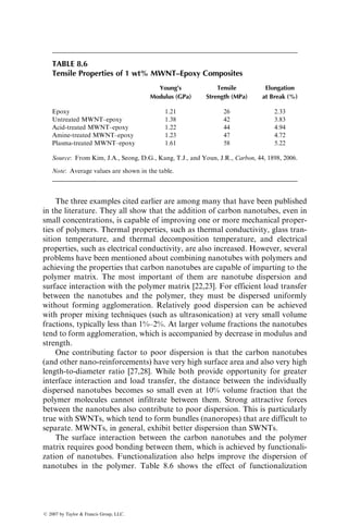
![The in situ method is commonly used with thermoset polymers, such as
epoxy. It has also been used with thermoplastics, such as polystyrene
and polyamide-6 (PA-6), and elastomers, such as polyurethane and
thermoplastic polyolefins (TPOs). The first important commercial appli-
cation of nanoclay composite was based on polyamide-6, and as dis-
closed by its developer, Toyota Motor Corp., it was prepared by the
in situ method [2]. In this case, the montmorillonite clay was mixed with
an a,v-amino acid in aqueous hydrochloric acid to attach carboxyl
groups to the clay particles. The modified clay was then mixed with
the caprolactam monomer at 1008C, where it was swollen by the mono-
mer. The carboxyl groups initiated the ring-opening polymerization
reaction of caprolactam to form polyamide-6 molecules and ionically
bonded them to the clay particles. The growth of the molecules caused
the exfoliation of the clay particles.
3. Melt processing method: The layered silicate particles are mixed with the
polymer in the liquid state. Depending on the processing condition and
the compatibility between the polymer and the clay surface, the polymer
molecules can enter into the interlayer space of the clay particles and can
form either an intercalated or an exfoliated structure.
The melt processing method has been used with a variety of thermoplastics,
such as polypropylene and polyamide-6, using conventional melt processing
techniques, such as extrusion and injection molding. The high melt viscosity of
thermoplastics and the mechanical action of the rotating screw in an extruder
or an injection-molding machine create high shear stresses which tend to
delaminate the original clay stack into thinner stacks. Diffusion of polymer
molecules between the layers in the stacks then tends to peel the layers away
into intercalated or exfoliated form [3].
The ability of smectite clay to greatly improve mechanical properties of
polymers was first demonstrated in the research conducted by Toyota Motor
Corp. in 1987. The properties of the nanoclay–polyamide-6 composite prepared
by the in situ polymerization method at Toyota Research are given in Table 8.1.
With the addition of only 4.2 wt% of exfoliated montmorillonite nanoclay, the
tensile strength increased by 55% and the tensile modulus increased by 91%
compared with the base polymer, which in this case was a polyamide-6.
The other significant increase was in the heat deflection temperature (HDT).
Table 8.1 also shows the benefit of exfoliation as the properties with exfoliation
are compared with those without exfoliation. The nonexfoliated clay–PA-6
composite was prepared by simply melt blending montmorillonite clay with
PA-6 in a twin-screw extruder.
Since the publication of the Toyota research results, the development of
nanoclay-reinforced thermoplastics and thermosets has rapidly progressed.
ß 2007 by Taylor Francis Group, LLC.](https://image.slidesharecdn.com/fiberreinforcedcompositesmaterialsmanufacturinganddesignp1-220510152925-9ef3de0d/85/Fiber_Reinforced_Composites_Materials_Manufacturing_and_Design_P-1-pdf-593-320.jpg)
![The most attractive attribute of adding nanoclay to polymers has been the
improvement of modulus that can be attained with only 1–5 wt% of nanoclay.
There are many other advantages such as reduction in gas permeability and
increase in thermal stability and fire retardancy [1,4]. The key to achieving
improved properties is the exfoliation. Uniform dispersion of nanoclay and
interaction between nanoclay and the polymer matrix are also important
factors, especially in controlling the tensile strength, elongation at break, and
impact resistance.
8.2 CARBON NANOFIBERS
Carbon nanofibers are produced either in vapor-grown form [5] or by electro-
spinning [6]. Vapor-grown carbon nanofibers (VGCNF) have so far received the
most attention for commercial applications and are discussed in this section.
They are typically 20–200 nm in diameter and 30–100 mm in length. In com-
parison, the conventional PAN or pitch-based carbon fibers are 5–10 mm in
diameter and are produced in continuous length. Carbon fibers are also made
in vapor-grown form, but their diameter is in the range of 3–20 mm.
VGCNF are produced in vapor phase by decomposing carbon-containing
gases, such as methane (CH4), ethane (C2H6), acetylene (C2H2), carbon mon-
oxide (CO), benzene, or coal gas in presence of floating metal catalyst particles
inside a high-temperature reactor. Ultrafine particles of the catalyst are either
carried by the flowing gas into the reactor or produced directly in the reactor by
the decomposition of a catalyst precursor. The most common catalyst is iron,
which is produced by the decomposition of ferrocene, Fe(CO)5. A variety of
other catalysts, containing nickel, cobalt, nickel–iron, and nickel–cobalt com-
pounds, have also been used. Depending on the carbon-containing gas, the
TABLE 8.1
Properties of Nanoclay-Reinforced Polyamide-6
Wt%
of Clay
Tensile
Strength
(MPa)
Tensile
Modulus
(GPa)
Charpy Impact
Strength
(kJ=m2
)
HDT (8C)
at 145 MPa
Polyamide-6
(PA-6)
0 69 1.1 2.3 65
PA-6 with exfoliated
nanoclay
4.2 107 2.1 2.8 145
PA-6 with
nonexfoliated clay
5.0 61 1.0 2.2 89
Source: Adapted from Kato, M. and Usuki, A., in Polymer–Clay Nanocomposites, T.J. Pinnavai
and G.W. Beall, eds., John Wiley Sons, Chichester, UK, 2000.
ß 2007 by Taylor Francis Group, LLC.](https://image.slidesharecdn.com/fiberreinforcedcompositesmaterialsmanufacturinganddesignp1-220510152925-9ef3de0d/85/Fiber_Reinforced_Composites_Materials_Manufacturing_and_Design_P-1-pdf-594-320.jpg)
![decomposition temperature can range up to 12008C. The reaction is conducted
in presence of other gases, such as hydrogen sulfide and ammonia, which act as
growth promoters. Cylindrical carbon nanofibers grow on the catalyst particles
and are collected at the bottom of the reactor. Impurities on their surface,
such as tar and other aromatic hydrocarbons, are removed by a subsequent
process called pyrolitic stripping, which involves heating them to about 10008C
in a reducing atmosphere. Heat treatment at temperatures up to 30008C is used
to graphitize their surface and achieve higher tensile strength and tensile
modulus. However, the optimum heat treatment temperature for maximum
mechanical properties is found to be close to 15008C [5].
The diameter of carbon nanofibers and the orientation of graphite layers in
carbon nanofibers with respect to their axis depend on the carbon-containing
gas, the catalyst type, and the processing conditions, such as gas flow rate and
temperature [7,8]. The catalyst particle size also influences the diameter.
Several different morphologies of carbon nanofibers have been observed
[8,9]: platelet, in which the graphite layers are stacked normal to the fiber axis;
hollow tubular construction, in which the graphite layers are parallel to the fiber
axis, and fishbone or herringbone (with or without a hollow core), in which
graphite layers are at an angle between 108 and 458 with the fiber axis (Figure
8.3). Single-wall and double-wall morphologies have been observed in heat-
treated carbon nanofibers [10]. Some of the graphite layers in both single-wall
and double-wall morphologies are folded, the diameter of the folds remaining
close to 1 nm.
Table 8.2 lists the properties of a commercial carbon nanofiber (Pyrograf
III) (Figure 8.4) as reported by its manufacturer (Applied Sciences, Inc.). The
tensile modulus value listed in Table 8.2 is 600 GPa; however it should be noted
that owing to the variety of morphologies observed in carbon nanofibers, they
exhibit a range of modulus values, from as low as 110 GPa to as high as 700
GPa. Studies on vapor-grown carbon fibers (VGCF) [11], which are an order of
(a) (b) (c) (d) (e) (f)
FIGURE 8.3 Different morphologies of carbon nanofibers. (a) Graphite layers stacked
normal to the fiber axis; (b) Hollow tubular construction with graphite layers parallel
to the fiber axis; (c) and (d) Fishbone or herringbone morphology with graphite layers
at an angle with the fiber axis; (e) Fishbone morphology with end loops; and (f) Double-
walled morphology.
ß 2007 by Taylor Francis Group, LLC.](https://image.slidesharecdn.com/fiberreinforcedcompositesmaterialsmanufacturinganddesignp1-220510152925-9ef3de0d/85/Fiber_Reinforced_Composites_Materials_Manufacturing_and_Design_P-1-pdf-595-320.jpg)
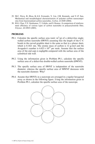
![In general, incorporation of carbon nanofibers in thermoplastics has shown
modest to high improvement in modulus and strength, whereas their incorpor-
ation in thermosets has shown relatively smaller improvements. An example of
each is given as follows.
Finegan et al. [12] conducted a study on the tensile properties of carbon
nanofiber-reinforced polypropylene. The nanofibers were produced with a variety
of processing conditions (different carbon-containing gases, different gas flow
rates, with and without graphitization). A variety of surface treatments were
applied on the nanofibers. The composite tensile specimens with 15 vol% nanofi-
bers were prepared using melt processing (injection molding). In all cases, they
observed an increase in both tensile modulus and strength compared with poly-
propylene itself. However, the amount of increase was influenced by the nanofiber
production condition and the surface treatment. When the surface treatment
involved surface oxidation in a CO2 atmosphere at 8508C, the tensile modulus
and strength of the composite were 4 GPa and 70 MPa, respectively, both of which
were greater than three times the corresponding values for polypropylene.
Patton et al. [13] reported the effect of carbon nanofiber addition to epoxy.
The epoxy resin was diluted using acetone as the solvent. The diluted epoxy was
then infused into the carbon nanofiber mat. After removing the solvent, the
epoxy-soaked mat was cured at 1208C and then postcured. Various nanofiber
surface treatments were tried. The highest improvement in flexural modulus
and strength was observed with carbon nanofibers that were heated in air at
4008C for 30 min. With ~18 vol% of carbon nanofibers, the flexural modulus of
the composite was nearly twice that of epoxy, but the increase in flexural
strength was only about 36%.
8.3 CARBON NANOTUBES
Carbon nanotubes were discovered in 1991, and within a short period of time,
have attracted a great deal of research and commercial interest due to their
potential applications in a variety of fields, such as structural composites,
energy storage devices, electronic systems, biosensors, and drug delivery sys-
tems [14]. Their unique structure gives them exceptional mechanical, thermal,
electrical, and optical properties. Their elastic modulus is reported to be 1
TPa, which is close to that of diamond and 3–4 times higher than that of carbon
fibers. They are thermally stable up to 28008C in vacuum; their thermal con-
ductivity is about twice that of diamond and their electric conductivity is 1000
times higher than that of copper.
8.3.1 STRUCTURE
Carbon nanotubes are produced in two forms, single-walled nanotubes
(SWNT) and multiwalled nanotubes (MWNT). SWNT is a seamless hollow
cylinder and can be visualized as formed by rolling a sheet of graphite layer,
ß 2007 by Taylor Francis Group, LLC.](https://image.slidesharecdn.com/fiberreinforcedcompositesmaterialsmanufacturinganddesignp1-220510152925-9ef3de0d/85/Fiber_Reinforced_Composites_Materials_Manufacturing_and_Design_P-1-pdf-597-320.jpg)
![whereas MWNT consists of a number of concentric SWNT. Both SWNT
and MWNT are closed at the ends by dome-shaped caps. The concentric
SWNTs inside an MWNT are also end-capped. The diameter of an SWNT is
typically between 1 and 1.4 nm and its length is between 50 and 100 mm. The
specific surface area of an SWNT is 1315 m2
=g, and is independent of its
diameter [15]. The outer diameter of an MWNT is between 1.4 and 100 nm.
The separation between the concentric SWNT cylinders in an MWNT is about
3.45 A8, which is slightly greater than the distance between the graphite layers
in a graphite crystal. The specific surface area of an MWNT depends on the
number of walls. For example, the specific surface area of a double-walled
nanotube is between 700 and 800 m2
=g and that of a 10-walled nanotube is
about 200 m2
=g [15].
The structure of an SWNT depends on how the graphite sheets is rolled up
and is characterized by its chirality or helicity, which is defined by the chiral
angle and the chiral vector (Figure 8.5). The chiral vector is written as
Ch ¼ na1 þ ma2, (8:1)
Zigzag direction
(0,0)
(1,1) Ch
(3,0)
(2,2)
a1
a2
(3,3)
(4,4)
(5,5)
Armchair direction
(7,4)
(6,3)
(4,2) (5,2) (7,2) (8,2)
(4,0) (6,0)
θ (8,0)
(8,1)
(9,0)
FIGURE 8.5 Chiral vector and chiral angle. (From Govindaraj, A. and Rao, C.N.R.,
The Chemistry of Nanomaterials, Vol. 1, C.N.R. Rao, A. Müller, and A.K. Cheetham,
eds., Wiley-VCH, KGaA, Germany, 2004. With permission.)
ß 2007 by Taylor Francis Group, LLC.](https://image.slidesharecdn.com/fiberreinforcedcompositesmaterialsmanufacturinganddesignp1-220510152925-9ef3de0d/85/Fiber_Reinforced_Composites_Materials_Manufacturing_and_Design_P-1-pdf-598-320.jpg)
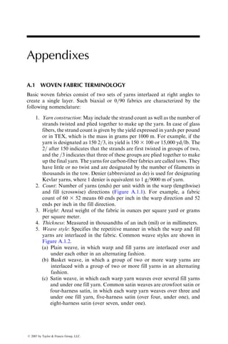
![and 0
u 30
. The diameter of the nanotube is given by
d ¼
ao
ffiffiffi
3
p
p
ffiffiffiffiffiffiffiffiffiffiffiffiffiffiffiffiffiffiffiffiffiffiffiffiffiffiffiffi
m2 þ mn þ n2
p
, (8:3)
where ao ¼ C–C bond length, which is equal to 1.42 Å.
The chirality of a carbon nanotube has a significant influence on its electrical
and mechanical properties. Depending on the chirality, a carbon nanotube can
behave either as a metallic material or a semiconducting material. For example,
armchair nanotubes are metallic; nanotubes with (nm) ¼ 2k, where k is a
nonzero integer, are semiconductors with a tiny band gap, and all other nano-
tubes are semiconductors with a band gap that inversely varies with the nanotube
diameter. Chirality also controls the deformation characteristics of carbon
nanotubes subjected to tensile stresses and therefore, determines whether they
will fracture like a brittle material or deform like a ductile material [16].
The current processing methods used for making carbon nanotubes intro-
duce two types of defect in their structures: topological defects and structural
defects. The examples of topological defects are pentagonal and heptagonal
arrangements of carbon atoms, which may be mixed with the hexagonal arrange-
ments. The structural defects include nontubular configurations, such as cone-
shaped end caps, bent shapes, branched construction with two or more tubes
connected together, and bamboo-like structure in which several nanotubes are
joined in the lengthwise direction. In general, MWNTs contain more defects
than SWNTs.
Carbon nanotubes can form secondary structures. One of these secondary
structures is the SWNT rope or bundle, which is a self-assembled close-
packed array of many (often thousands or more) SWNTs. The self-assembly
occurs at the time of forming the SWNTs, due to the attractive forces between
them arising from binding energy of 500–900 eV=nm. If the arrangement
of SWNTs in the array is well ordered (e.g., with hexagonal lattice structure),
it is called a rope. If the arrangement of SWNTs is not ordered, it is called
a bundle [17].
8.3.2 PRODUCTION OF CARBON NANOTUBES
There are three main methods for producing carbon nanotubes: electric arc
discharge, laser ablation, and chemical vapor deposition (CVD) [18]. The
quantity of production of carbon nanotubes by the first two methods is
relatively small. Since CVD can produce larger quantities of carbon nanotubes
and is more versatile, it has become the focus of attention for industrial
production and several different variations of the basic CVD process
(e.g., plasma-enhanced CVD or PECVD process and high-pressure carbon
monoxide or HiPco process) have been developed. However, the structure of
nanotubes produced by CVD is usually different from that of nanotubes
ß 2007 by Taylor Francis Group, LLC.](https://image.slidesharecdn.com/fiberreinforcedcompositesmaterialsmanufacturinganddesignp1-220510152925-9ef3de0d/85/Fiber_Reinforced_Composites_Materials_Manufacturing_and_Design_P-1-pdf-600-320.jpg)
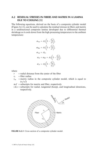
![Liquid phase purification involves refluxing in an acid such as nitric acid at an
elevated temperature. In general, carbon nanotubes produced by the arc dis-
charge process requires more extensive purification than the other two processes.
Carbon nanotubes are often formed as long, entangled bundles. The ‘‘cut-
ting’’ process is used to shorten their lengths, disentangle them, open up the
ends, and provide active sites for functionalization. The cutting process can be
either mechanical (e.g., by ball-milling) or chemical (e.g., by treating them in a
3:1 mixture of concentrated sulfuric acid and nitric acid).
Carbon nanotubes are available in a variety of forms. One of these forms is
called the bucky paper, which is a thin film of randomly oriented SWNTs. It is
made by filtering SWNTs dispersed in an aqueous or organic solution and then
peeling off the nanotube film from filter paper. Carbon nanotube fibers and
yarns containing aligned SWNTs have also been produced [19].
8.3.3 FUNCTIONALIZATION OF CARBON NANOTUBES
Carbon nanotubes are functionalized for a variety of purposes. Among them
are (1) improve their dispersion in the polymer matrix, (2) create better bonding
with the polymer matrix, and (3) increase their solubility in solvents. Functio-
nalization has also been used for joining of nanotubes to form a network
structure.
Functionalization can occur either at the defect sites on the nanotube wall
or at the nanotube ends. The functional groups are covalently bonded to the
nanotubes using either oxidation, fluorination, amidation, or other chemical
reactions. Functionalization can also be achieved using noncovalent inter-
actions, for example, by wrapping the nanotubes with polymer molecules or
adsorption of polymer molecules in the nanotubes. The covalent functionaliza-
tion is generally considered to provide better load transfer between the nano-
tubes and the surrounding polymer matrix, and therefore, improved
mechanical properties. On the other hand, noncovalent functionalization may
be preferred if it is required that the electronic characteristics of carbon nano-
tubes remain unchanged.
The covalent bonds can be produced in two different ways: (1) by direct
attachment of functional groups to the nanotubes and (2) by a two-step
functionalization process in which the nanotubes are chemically treated first
to attach simple chemical groups (e.g., –COOH and –OH) at the defect sites or
at their ends (Figure 8.7), which are later substituted with more active organic
groups. Carbon nanotubes have also been functionalized using silane-coupling
agents [20]. Silane-coupling agents are described in Chapter 2.
A variety of chemical and electrochemical functionalization processes have
been developed [15]. One of these processes is a two-step functionalization
process in which acidic groups, such as the carboxylic (–COOH) groups or
the hydroxyl (–OH) groups, are first attached by refluxing carbon nanotubes in
concentrated HNO3 or a mixture of H2SO4 and HNO3. One problem in acid
ß 2007 by Taylor Francis Group, LLC.](https://image.slidesharecdn.com/fiberreinforcedcompositesmaterialsmanufacturinganddesignp1-220510152925-9ef3de0d/85/Fiber_Reinforced_Composites_Materials_Manufacturing_and_Design_P-1-pdf-602-320.jpg)
![modulus of MWNT is higher than that of SWNT due to contributions from
the van der Waals forces between the concentric SWNTs in MWNT [14].
Experimental determination of the mechanical properties of carbon nano-
tubes is extremely difficult and has produced a variety of results. Several
investigators have used atomic force microscope (AFM) to determine the
Young’s modulus and strength. The Young’s modulus of MWNT determined
on AFM has ranged from 0.27 to 1.8 TPa and that of SWNT ranges from 0.32
to 1.47 TPa. Similarly, the strength of MWNT ranges from 11 to 63 GPa and
that of SWNT from 10 to 52 GPa. In the TPM experiments, the carbon
nanotubes have also shown high tensile strain (up to 15%) before fracture. It
has also been observed that carbon nanotubes exhibit nonlinear elastic deform-
ation under tensile, bending, as well as twisting loads. At high strains, they tend
to buckle of the wall.
The large variation in Young’s modulus and strength is attributed to the fact
that nanotubes produced by the current production methods may vary in length,
diameter, number of walls, chirality, and even atomic structure [21]. Further-
more, nanotubes produced by different methods contain different levels of
defects and impurities, which influence their mechanical properties. For
example, the Young’s modulus of CVD-produced MWNTs is found to be an
order of magnitude lower than that of the arc-discharged MWNTs, which is due
to the presence of higher amount of defects in the CVD-produced MWNTs.
8.3.5 CARBON NANOTUBE–POLYMER COMPOSITES
The three principal processing methods for combining carbon nanotubes with
polymer matrix [22,23] are (1) in situ polymerization, (2) solution processing,
and (3) melt processing.
1. In Situ Polymerization: In this process, the nanotubes are first dispersed
in the monomer and then the polymerization reaction is initiated to
transform the monomer to polymer. Depending on the polymer formed
and the surface functionality of the nanotubes, the polymer molecules
are either covalently bonded to the nanotubes or wrapped around the
nanotubes at the completion of the polymerization reaction.
2. Solution Processing: In this process, the nanotubes are mixed with a
polymer solution, which is prepared by dissolving the polymer in a
suitable solvent. The mixing is done using magnetic stirring, high shear
mixing, or sonication. The dispersion of the nanotubes in the solution
can be improved by treating them with a surfactant, such as derivatives
of sodium dodecylsulfate. The solution is poured in a casting mold and
the solvent is allowed to evaporate. The resulting material is a cast film
or sheet of carbon nanotube-reinforced polymer.
3. Melt Processing: Melt processing is the preferred method for incorpor-
ating carbon nanotubes in thermoplastics, particularly for high volume
ß 2007 by Taylor Francis Group, LLC.](https://image.slidesharecdn.com/fiberreinforcedcompositesmaterialsmanufacturinganddesignp1-220510152925-9ef3de0d/85/Fiber_Reinforced_Composites_Materials_Manufacturing_and_Design_P-1-pdf-604-320.jpg)
![applications. It has been used with a variety of thermoplastics, such as
high-density polyethylene, polypropylene, polystyrene, polycarbonate,
and polyamide-6. In this process, the nanotubes are blended with the
liquid polymer in a high shear mixer or in an extruder. The blend is then
processed to produce the final product using injection molding, extru-
sion, or compression molding. It is important to note that the addition
of carbon nanotubes increases the viscosity of the liquid polymer, and
therefore, proper adjustments need to be made in the process parameters
to mold a good product.
Carbon nanotubes have also been used with thermoset polymers such as epoxy
and vinyl ester. They are dispersed in the liquid thermoset prepolymer using
sonication. After mixing the blend with a hardener or curing initiator, it is
poured into a casting mold, which is then heated to the curing temperature.
Curing can be conducted in vacuum to reduce the void content in the compos-
ite. To improve the dispersion of the nanotubes, the viscosity of the thermoset
prepolymer can be reduced with a solvent that can be evaporated later.
8.3.6 PROPERTIES OF CARBON NANOTUBE–POLYMER COMPOSITES
Based on the mechanical properties of carbon nanotubes described in Section
8.3.4, it is expected that the incorporation of carbon nanotubes in a polymer
matrix will create composites with very high modulus and strength. Indeed,
many studies have shown that with proper dispersion of nanotubes in the
polymer matrix, significant improvement in mechanical properties can be
achieved compared with the neat polymer. Three examples are given as follows.
In the first example, CVD-produced MWNTs were dispersed in a toluene
solution of polystyrene using an ultrasonic bath [24]. The mean external
diameter of the MWNTs was 30 nm and their length was between 50 and 55
mm. No functionalization treatments were used. MWNT-reinforced polystyr-
ene film was produced by solution casting. Tensile properties of the solution
cast films given in Table 8.4 show that both elastic modulus and tensile
strength increased with increasing MWNT weight fraction. With the addition
of 5 wt% MWNT, the elastic modulus of the composite was 120% higher and
the tensile strength was 57% higher than the corresponding properties of
polystyrene.
The second example involves melt-processed MWNT-reinforced poly-
amide-6 [25]. The MWNTs, in this example, was also prepared by CVD and
functionalized by treating them in nitric acid. The MWNTs and polyamide-6
were melt-compounded in a twin-screw mixer and film specimens were prepared
by compression molding. The MWNT content in the composite was 1 wt%. As
shown in Table 8.5, both tensile modulus and strength of the composite were
significantly higher compared with the tensile modulus and strength of poly-
amide-6. However, the elongation at break was decreased.
ß 2007 by Taylor Francis Group, LLC.](https://image.slidesharecdn.com/fiberreinforcedcompositesmaterialsmanufacturinganddesignp1-220510152925-9ef3de0d/85/Fiber_Reinforced_Composites_Materials_Manufacturing_and_Design_P-1-pdf-605-320.jpg)
![The final example considers the tensile properties of 1 wt% MWNT-
reinforced epoxy [26]. The MWNT, in this case, was produced by the CVD
process, and had an average diameter of 13 nm and an average length of 10 mm.
They were acid-treated in a 3:1 mixture of 65% H2SO4 and HNO3 for 30 min at
1008C to remove the impurities. The acid-treated nanotubes were then sub-
jected to two different functionalization treatments: amine treatment and
plasma oxidation. The acid-treated and amine-treated MWNTs were first
mixed with ethanol using a sonicator and then dispersed in epoxy. The
plasma-oxidized MWNTs were dispersed directly in epoxy. The composite
was prepared by film casting. As shown in Table 8.6, the addition of MWNT
caused very little improvement in modulus, but tensile strength and elongation
at break were significantly improved.
TABLE 8.4
Tensile Properties of Cast MWNT–Polystyrene
Elastic
Modulus (GPa)
Tensile
Strength (MPa)
Polystyrene 1.53 19.5
Polystyrene þ 1 wt% MWNT 2.1 24.5
Polystyrene þ 2 wt% MWNT 2.73 25.7
Polystyrene þ 5 wt% MWNT 3.4 30.6
Source: From Safadi, B., Andrews, R., and Grulke, E.A., J. Appl.
Polym. Sci., 84, 2660, 2002.
Note: Average values are shown in the table.
TABLE 8.5
Tensile Properties of 1 wt% MWNT-Reinforced
Polyamide-6
Polyamide-6
1 wt% MWNT
1Polyamide-6
Tensile modulus (GPa) 0.396 0.852
Yield strength (MPa) 18 40.3
Elongation at break 150 125
Source: From Zhang, W.D., Shen, L., Phang, I.Y., and Liu, T.,
Macromolecules, 37, 256, 2004.
Note: Average values are shown in the table.
ß 2007 by Taylor Francis Group, LLC.](https://image.slidesharecdn.com/fiberreinforcedcompositesmaterialsmanufacturinganddesignp1-220510152925-9ef3de0d/85/Fiber_Reinforced_Composites_Materials_Manufacturing_and_Design_P-1-pdf-606-320.jpg)
![The three examples cited earlier are among many that have been published
in the literature. They all show that the addition of carbon nanotubes, even in
small concentrations, is capable of improving one or more mechanical proper-
ties of polymers. Thermal properties, such as thermal conductivity, glass tran-
sition temperature, and thermal decomposition temperature, and electrical
properties, such as electrical conductivity, are also increased. However, several
problems have been mentioned about combining nanotubes with polymers and
achieving the properties that carbon nanotubes are capable of imparting to the
polymer matrix. The most important of them are nanotube dispersion and
surface interaction with the polymer matrix [22,23]. For efficient load transfer
between the nanotubes and the polymer, they must be dispersed uniformly
without forming agglomeration. Relatively good dispersion can be achieved
with proper mixing techniques (such as ultrasonication) at very small volume
fractions, typically less than 1%–2%. At larger volume fractions the nanotubes
tend to form agglomeration, which is accompanied by decrease in modulus and
strength.
One contributing factor to poor dispersion is that the carbon nanotubes
(and other nano-reinforcements) have very high surface area and also very high
length-to-diameter ratio [27,28]. While both provide opportunity for greater
interface interaction and load transfer, the distance between the individually
dispersed nanotubes becomes so small even at 10% volume fraction that the
polymer molecules cannot infiltrate between them. Strong attractive forces
between the nanotubes also contribute to poor dispersion. This is particularly
true with SWNTs, which tend to form bundles (nanoropes) that are difficult to
separate. MWNTs, in general, exhibit better dispersion than SWNTs.
The surface interaction between the carbon nanotubes and the polymer
matrix requires good bonding between them, which is achieved by functionali-
zation of nanotubes. Functionalization also helps improve the dispersion of
nanotubes in the polymer. Table 8.6 shows the effect of functionalization
TABLE 8.6
Tensile Properties of 1 wt% MWNT–Epoxy Composites
Young’s
Modulus (GPa)
Tensile
Strength (MPa)
Elongation
at Break (%)
Epoxy 1.21 26 2.33
Untreated MWNT–epoxy 1.38 42 3.83
Acid-treated MWNT–epoxy 1.22 44 4.94
Amine-treated MWNT–epoxy 1.23 47 4.72
Plasma-treated MWNT–epoxy 1.61 58 5.22
Source: From Kim, J.A., Seong, D.G., Kang, T.J., and Youn, J.R., Carbon, 44, 1898, 2006.
Note: Average values are shown in the table.
ß 2007 by Taylor Francis Group, LLC.](https://image.slidesharecdn.com/fiberreinforcedcompositesmaterialsmanufacturinganddesignp1-220510152925-9ef3de0d/85/Fiber_Reinforced_Composites_Materials_Manufacturing_and_Design_P-1-pdf-607-320.jpg)
![of MWNTs. The effect of functionalization of SWNT is shown in Table 8.7,
which gives the tensile properties of functionalized SWNT-reinforced PVA. In
this case, the SWNTs were prepared by the arc discharge method and purified by
refluxing in an aqueous nitric acid solution. The nanotubes were then functio-
nalized with low-molecular-weight PVA [29] using N,N0
-dicyclohexyl carbodii-
mide-activated esterification reaction. The functionalized SWNTs were mixed
with a water solution of PVA and solution cast into 50–100 mm thick films. Both
Young’s modulus and yield strength were significantly higher with functiona-
lized SWNTs. The higher yield strength with 2.5 wt% functionalized SWNTs
compared with 2.5 wt% purified SWNTs (without functionalization) was attrib-
uted to deagglomeration of SWNT ropes into separate nanotubes, better dis-
persion of them in the PVA matrix, and wetting by PVA.
Another approach to improving the mechanical properties of carbon
nanotube-reinforced polymers is to align the nanotubes in the direction of stress.
This is a relatively difficult task if the common processing methods are used.
Flow-induced alignment of nanotubes is created by solution spinning, melt
spinning, or other similar methods to produce carbon nanotube-reinforced
polymer fiber or film. Mechanical stretching of carbon nanotube-
reinforced thin polymer films also tend to align the nanotubes in the direction
of stretching. Other methods of aligning carbon nanotubes in polymer matrix,
including the application of magnetic field, are described in Ref. [23].
The effect of alignment of nanotubes on the properties of carbon nanotube-
reinforced polymer fibers is demonstrated in Table 8.8. In this case, the polymer
was polyacrylonitrile (PAN) and the fibers were prepared by solution spinning
[30]. The carbon nanotube content was 5% by weight. All of the mechanical
properties, including strain-at-failure and toughness, increased with the add-
ition of SWNT, MWNT, as well as VGCNF. There was a significant decrease
TABLE 8.7
Tensile Properties of Functionalized SWNT-Reinforced Polyvinyl
Alcohol (PVA) Film
Material
Young’s
Modulus (GPa)
Yield
Strength (MPa)
Strain-to-Failure
(mm=mm)
PVA 4.0 83 0.60
PVA þ 2.5% purified SWNT 5.4 79 0.09
PVA þ 2.5% functionalized SWNT 5.6 97 0.05
PVA þ 5% functionalized SWNT 6.2 128 0.06
Source: From Paiva, M.C., Zhou, B., Fernando, K.A.S., Lin, Y., Kennedy, J.M., and Sun,
Y.-P., Carbon, 42, 2849, 2004.
Note: Average values are shown in the table.
ß 2007 by Taylor Francis Group, LLC.](https://image.slidesharecdn.com/fiberreinforcedcompositesmaterialsmanufacturinganddesignp1-220510152925-9ef3de0d/85/Fiber_Reinforced_Composites_Materials_Manufacturing_and_Design_P-1-pdf-608-320.jpg)
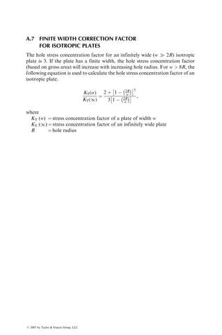
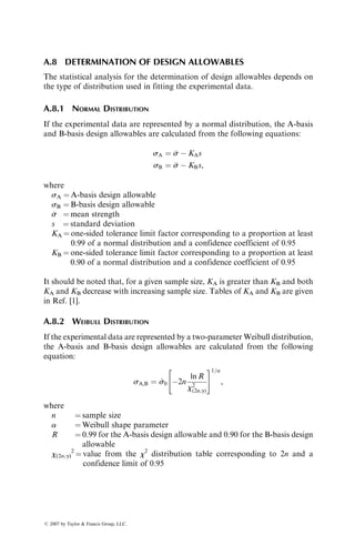
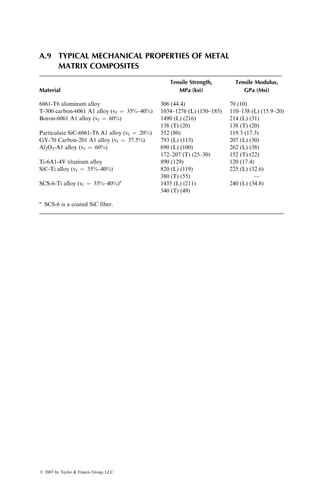
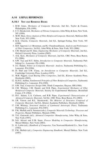
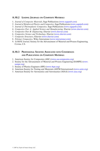
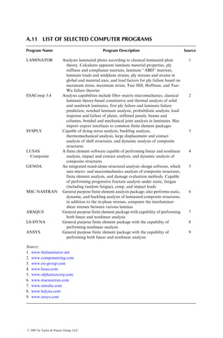
![A.2 RESIDUAL STRESSES IN FIBERS AND MATRIX IN A LAMINA
DUE TO COOLING [1]
The following equations, derived on the basis of a composite cylinder model
(Figure A.2.1), can be used to calculate the residual stresses in fibers and matrix
in a unidirectional composite lamina developed due to differential thermal
shrinkage as it cools down from the high processing temperature to the ambient
temperature:
srm ¼ A1 1
r2
m
r2
,
sum ¼ A1 1 þ
r2
m
r2
,
szm ¼ A2,
srf ¼ suf ¼ A1 1
r2
m
r2
f
,
szf ¼ A2 1
r2
m
r2
f
,
where
r ¼ radial distance from the center of the fiber
rf ¼ fiber radius
rm ¼ matrix radius in the composite cylinder model, which is equal to
(rf=vf
1
2)
m,f ¼ subscripts for matrix and fiber, respectively
r,u,z ¼ subscripts for radial, tangential (hoop), and longitudinal directions,
respectively.
Matrix
Fiber
rf
rm
Radial
T
a
n
g
e
n
t
i
a
l
q
FIGURE A.2.1 Cross section of a composite cylinder model.
ß 2007 by Taylor Francis Group, LLC.](https://image.slidesharecdn.com/fiberreinforcedcompositesmaterialsmanufacturinganddesignp1-220510152925-9ef3de0d/85/Fiber_Reinforced_Composites_Materials_Manufacturing_and_Design_P-1-pdf-616-320.jpg)


