FEA

1. Good Practices in Finite Element
Analysis (FEA)
Dr. Mahdi Damghani (2019-2020)
1

2. Learning Objectives
 Understanding of the pre-requisites to FEA
 Overview of the FEA build process
 Guidance on good practice in FEA
2

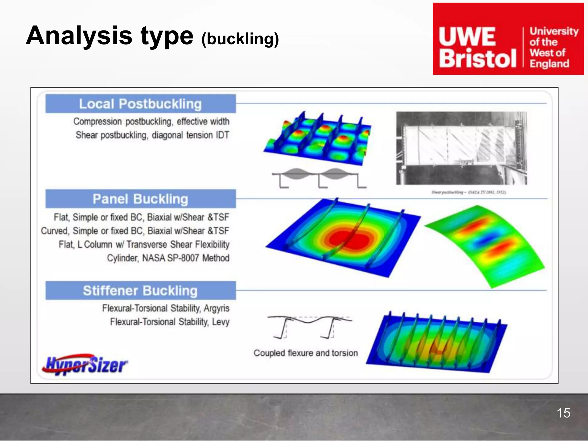
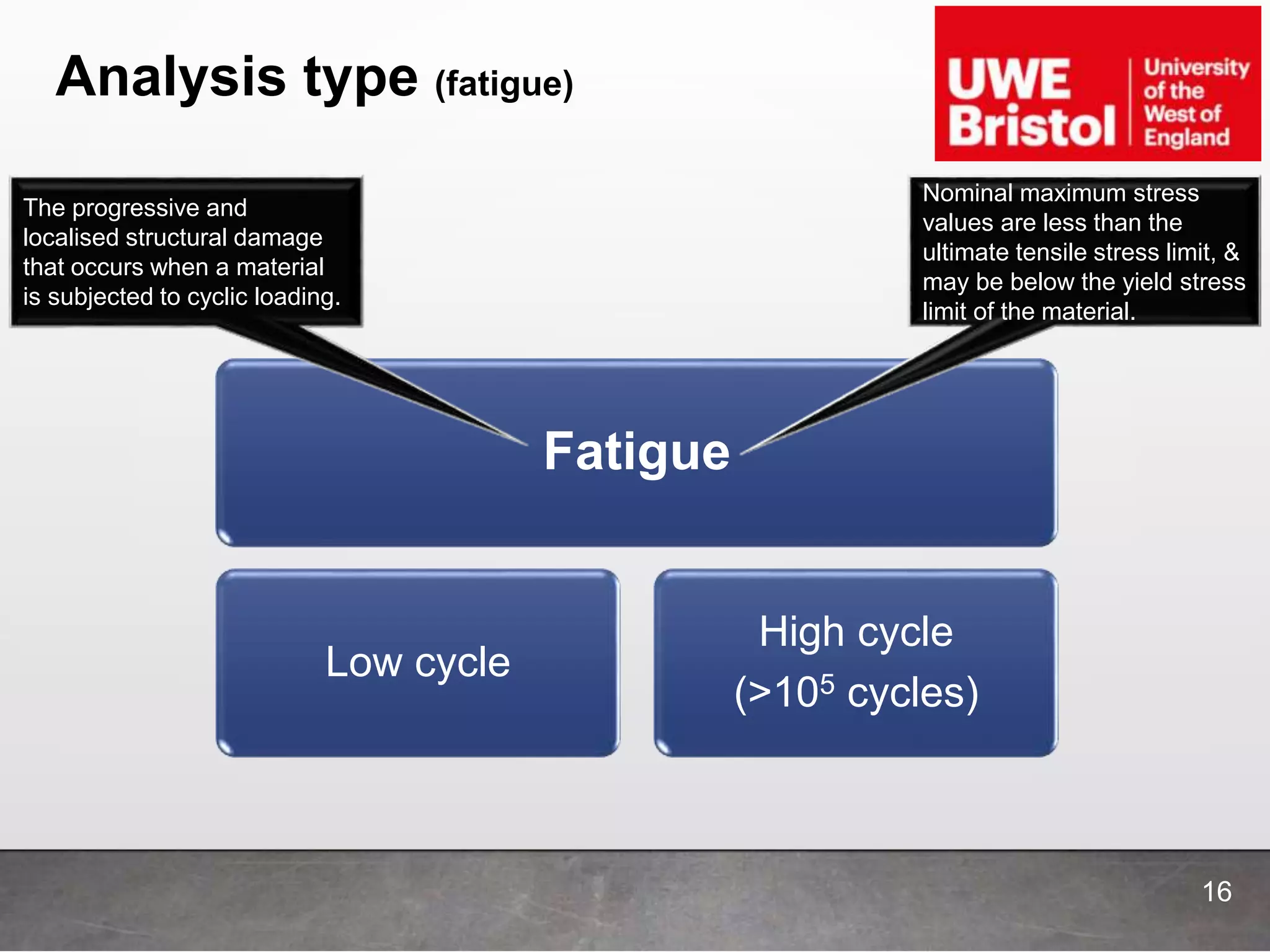
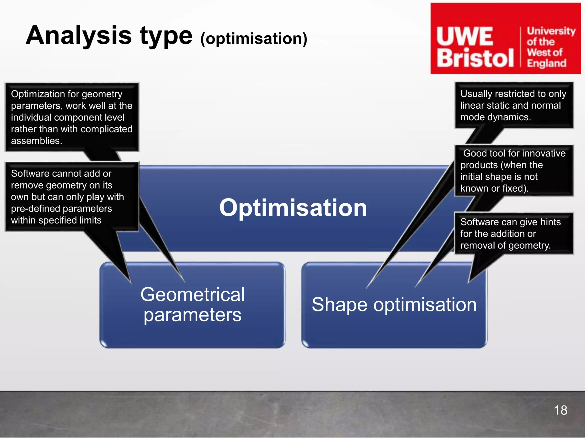
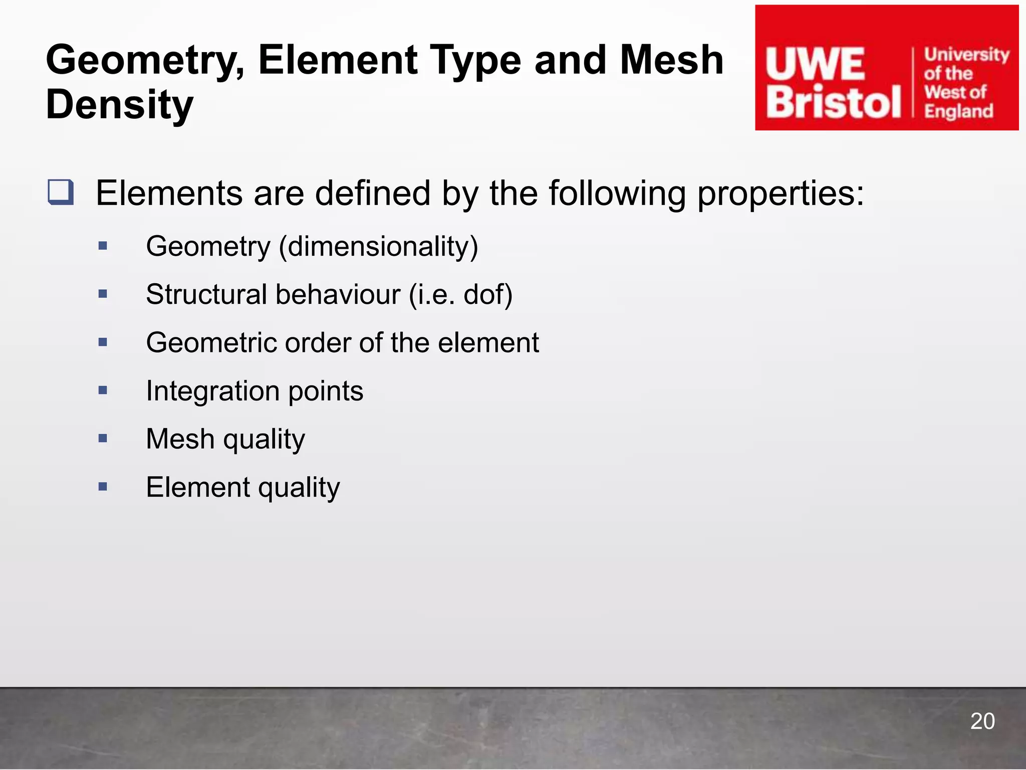
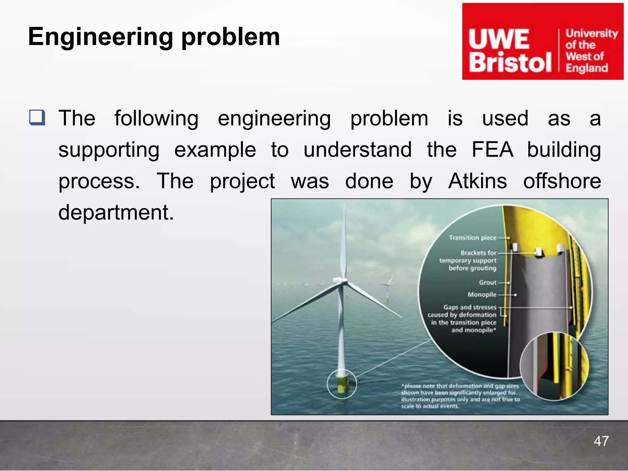
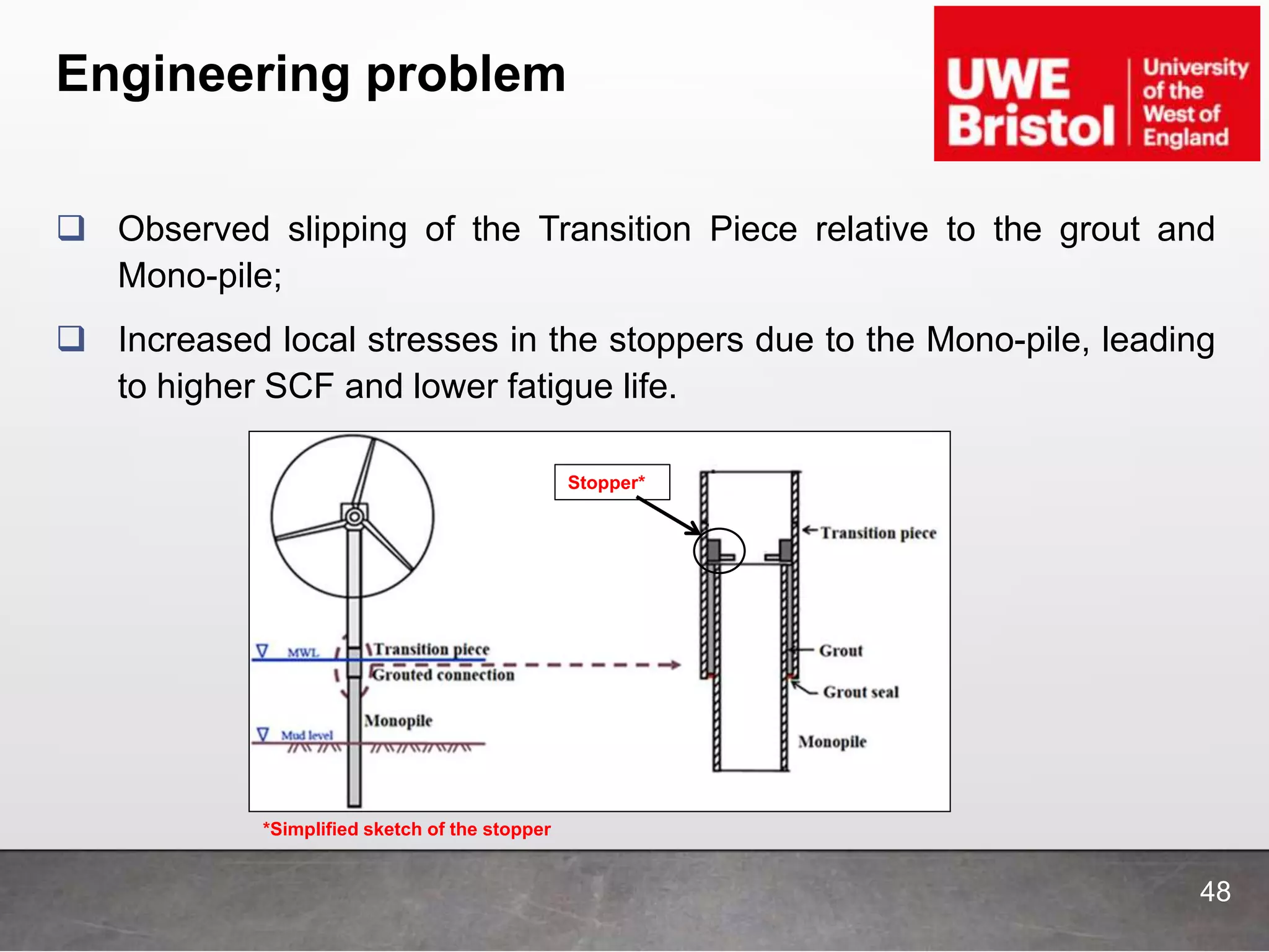
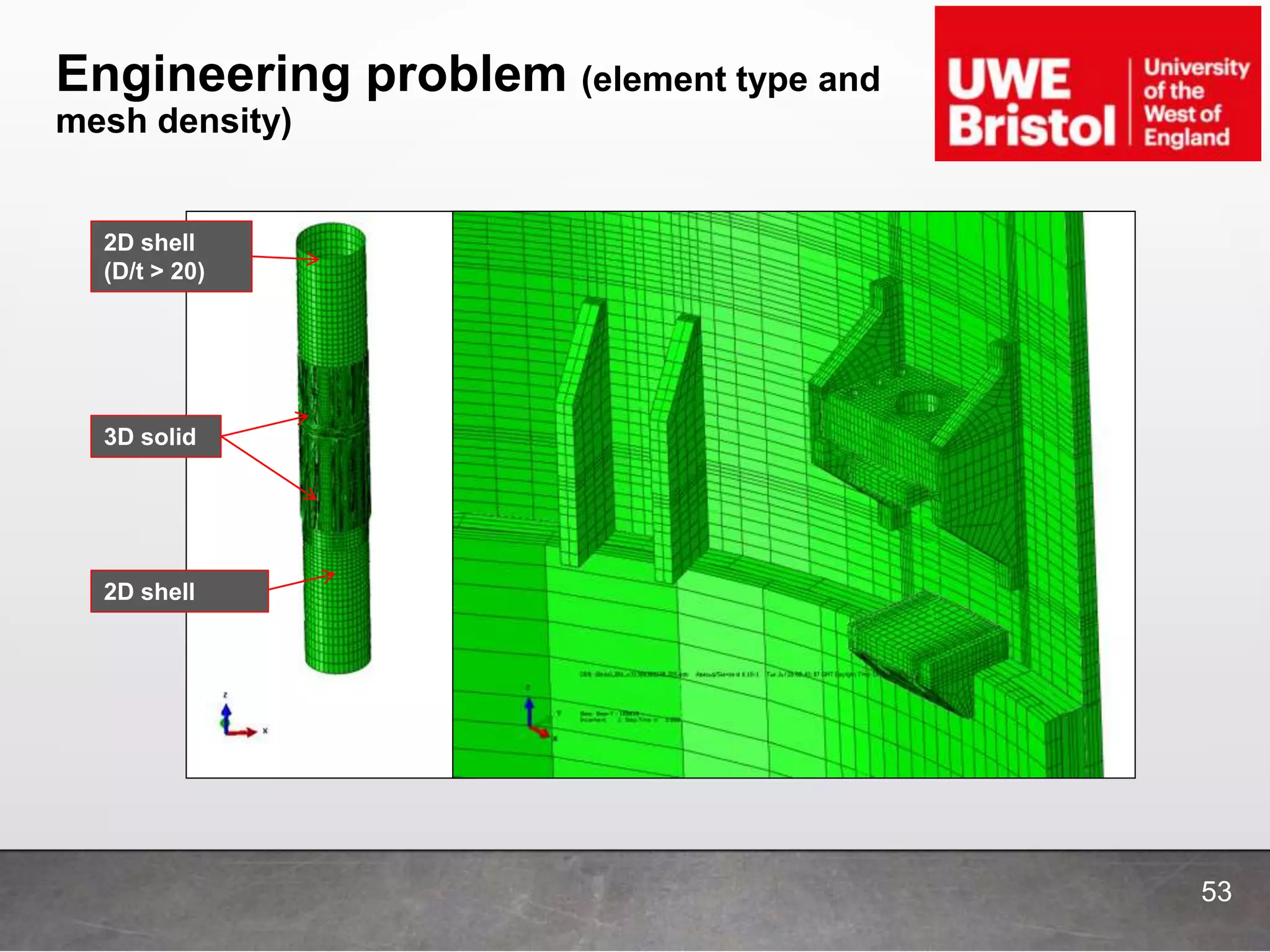
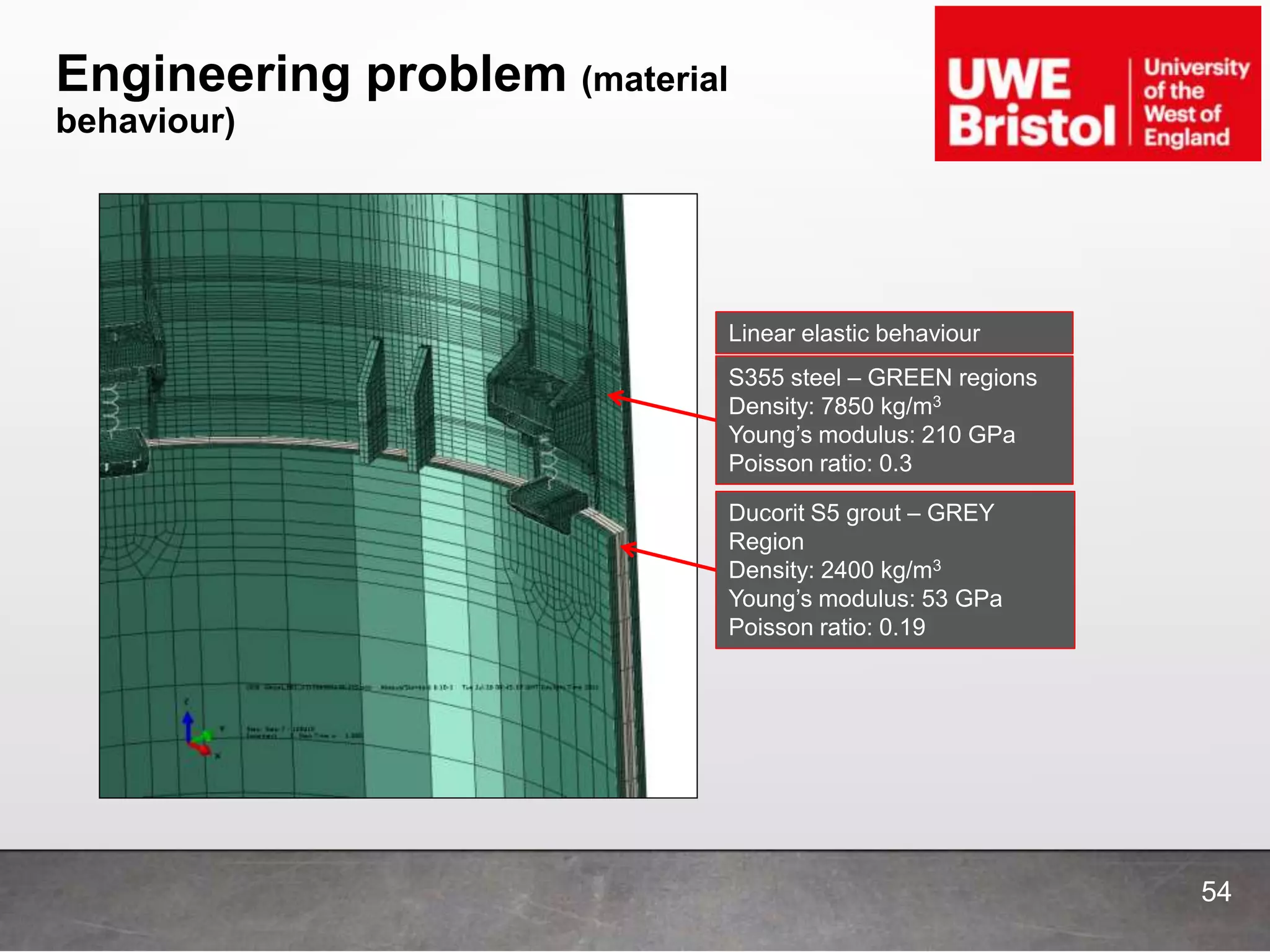
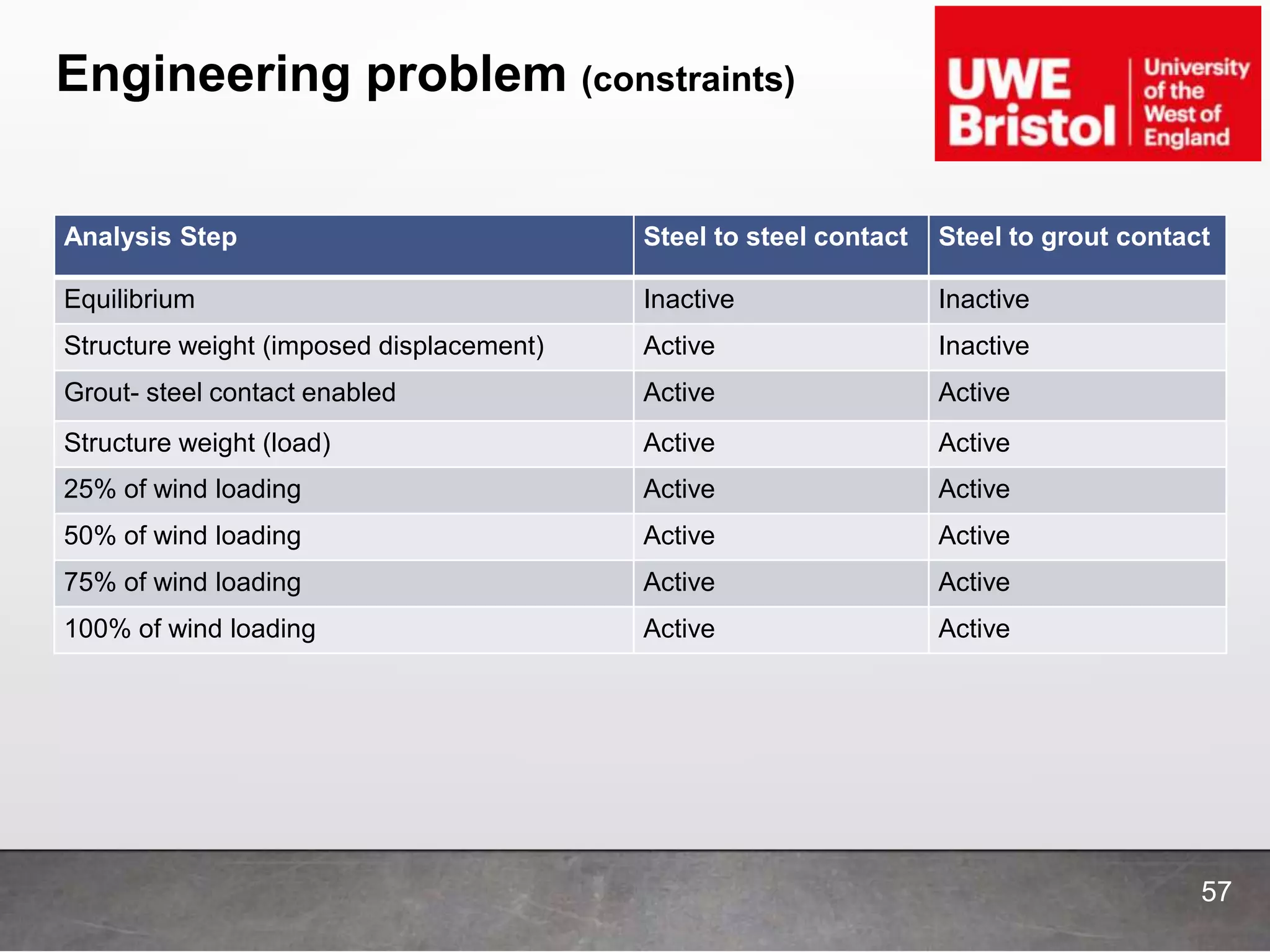
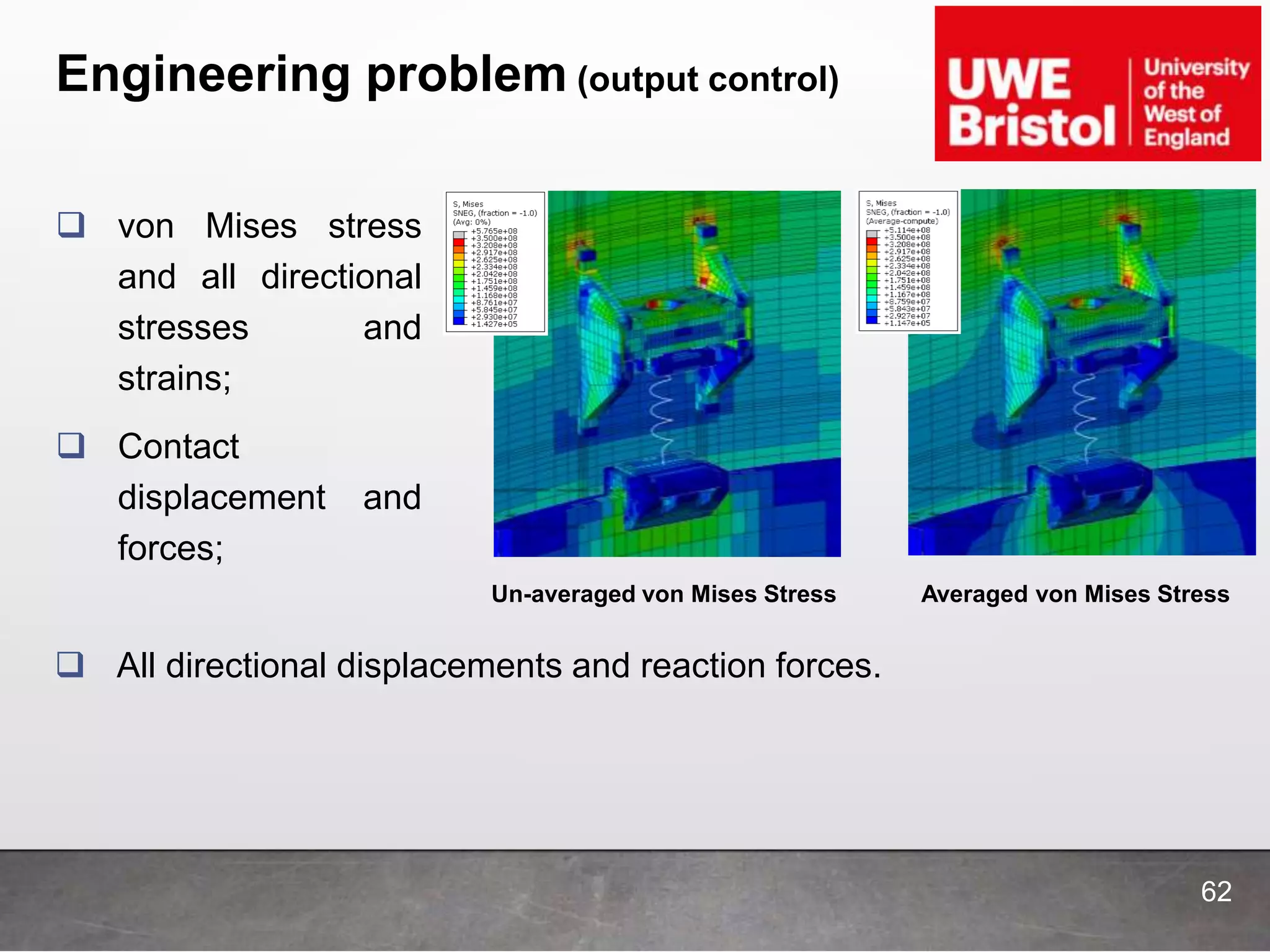
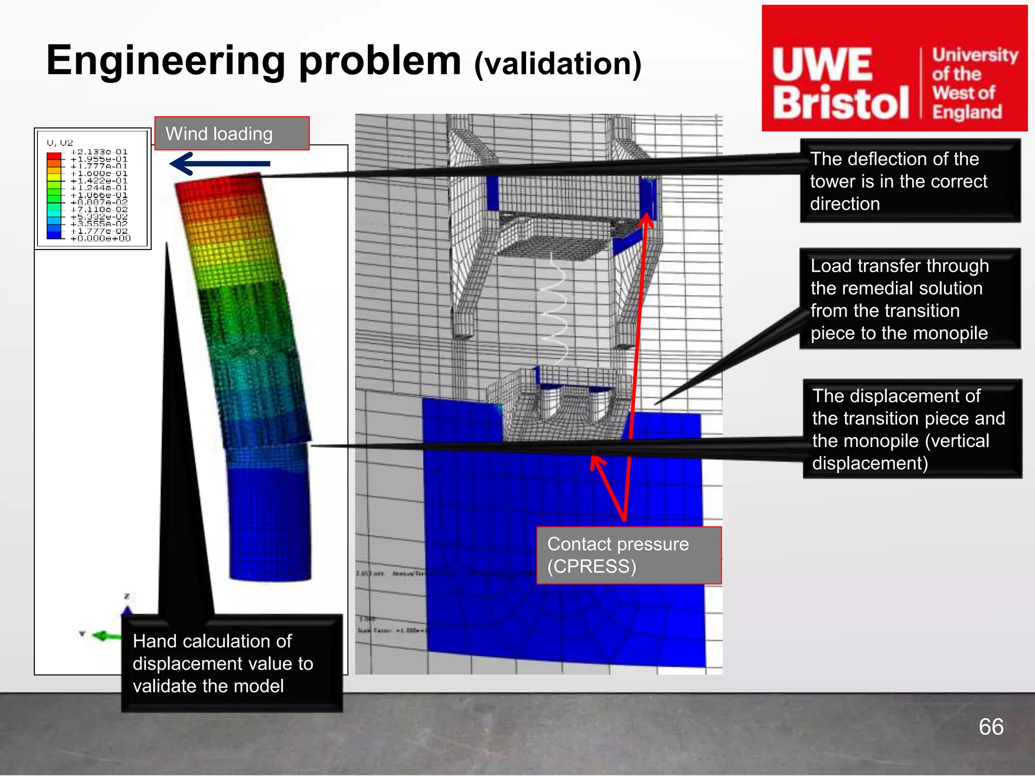
3. What is FEA?
 Finite Element Analysis is a method of breaking down a
physical structure into substructures called "finite
elements“;
 The finite elements and their interrelationships are
converted into equation form and solved mathematically.
3

4. Design process (traditional)
4
Design (CAD)
SolidWorks
Solid Edge
Catia
AutoCAD
Pro/E …
Virtual test
Abaqus
Radioss
Optistruct
NX Nastran
Ansys
LS-Dyna …
Build
Test
A lot of trial and
error and depends
highly on engineers
past experience and
knowledge

5. Design process (modern)
5
Conceive (optimisation)
Design (CAD)
SolidWorks
Solid Edge
Catia
AutoCAD
Pro/E …
Virtual test (CAE)
Radioss
Optistruct
Build
Test
Much faster and
more economical as
optimisation takes
place from very
beginning

6. Example of a modern design
process
6

7. Analysis type
 Linear static analysis
 Non-linear analysis
 Geometric nonlinearity
 Material nonlinearity
 Contact
 Dynamic analysis
 Buckling analysis
 Thermal analysis
 Fatigue analysis
 Optimisation
 CFD analysis
 Crash analysis
 NVH analysis
7

8. Analysis type
8
 Linear
 Linear means straight
line;
 The FE solver will
therefore always
follow a straight line
from base to
deformed state;
 An example in terms
of linear material
behaviour, σ =ε E.

9. Analysis type
9
 Static
 There is no variation of force
with respect to time;
 Equilibrium condition is valid;
 FEA solves the opposite
equation (non of the matrices
are time dependant).
0
0
0
x
y
z
F
F
F






0
0
0
x
y
z
M
M
M






/ 0
dF dt 
F = KD

10. Analysis type (nonlinear)
10
Nonlinear analysis
Geometric
Large
deformation
Material
Beyond
elastic limit
(metals)
Within
elastic limits
(non-
metals)
Creep (long
time
process)
Contact
Gap
elements
and contact
simulation
Stress strain
curve is
polynomial
Stiffness is
changing due
to change in
displacement
Stiffness is
changing due
to change in
displacement
Deals with true stress &
strain as opposed to
engineering stress & strain

11. Analysis type (nonlinear)
11
 Material nonlinearity;

12. Analysis type
12
      ( )
x x x t
not
  

M C K F
F KD

13. Analysis type (dynamic)
13
 Dynamic analysis vs. static analysis;
      ( )
x x x t
  
M C K F

14. Analysis type (buckling)
14
 Buckling (Eigenvalue analysis)
 For compressive loads only;
 Slender beams and sheet metal
parts;
 The output is critical buckling
load.

15. Analysis type (buckling)
15

16. Analysis type (fatigue)
16
Fatigue
Low cycle
High cycle
(>105 cycles)
The progressive and
localised structural damage
that occurs when a material
is subjected to cyclic loading.
Nominal maximum stress
values are less than the
ultimate tensile stress limit, &
may be below the yield stress
limit of the material.

17. Analysis type (fatigue)
17

18. Analysis type (optimisation)
18
Optimisation
Geometrical
parameters
Shape optimisation
Usually restricted to only
linear static and normal
mode dynamics.
Good tool for innovative
products (when the
initial shape is not
known or fixed).
Software can give hints
for the addition or
removal of geometry.
Optimization for geometry
parameters, work well at the
individual component level
rather than with complicated
assemblies.
Software cannot add or
remove geometry on its
own but can only play with
pre-defined parameters
within specified limits

19. Analysis type (optimisation)
19
 The design variable of a topology optimization is the
elements density (figure below);
 The design variable of a size optimisation is the
thickness of a sheet metal.

20. Geometry, Element Type and Mesh
Density
 Elements are defined by the following properties:
 Geometry (dimensionality)
 Structural behaviour (i.e. dof)
 Geometric order of the element
 Integration points
 Mesh quality
 Element quality
20

21. Geometry
21
 1D Line – 2D Plate – 3D Solid

22. Element type – Structural
behaviour (1D Elements)
-Truss/Rod/Bar elements;
-3 translational dof at each node
-Transmit axial force only
-Beam elements;
-6 dof at each node
-I-J defines element geometry
-I-K defines the beam normal
22

23. Element type – Structural
behaviour (2D Elements)
Plate element;
1 out of plane translation dof
2 in-plane axes rotation dof
Membrane element;
2 in-plane translation dof
Shell element;
3 translation dof
2 in-plane axes rotation dof
2D elements can be either
quadrilaterals or triangular
23

24. Element type – Structural
behaviour (2D Elements)
24
 It is best to minimise the use of triangular elements to less than 5% of
total elements;
 Why does FEA provide triangular elements?
 Mesh transition:
• In structural and fatigue analysis, rather than a uniform mesh, what helps is a small element
size in the critical areas and a coarse mesh or bigger elements in general areas. This type
of mesh gives good accuracy with manageable dofs. Trias help in creating a smooth mesh
transition from a dense mesh to a coarse mesh.
 Complex geometry:
• Geometry features like rib ends or sharp cut-outs demand for the use of triangular elements.
If quads are used instead of trias, then it will result in poor quality elements.
 Better mesh flow:
• For crash or nonlinear analysis, systematic mesh flow lines where all the elements satisfy
the required quality parameters is very important. Using a mix-mode element type instead of
pure quad element type helps to achieve better flow lines and convergence of solution.
 Tetra meshing & Mould flow analysis .

25. Element type – Structural
behaviour (3D Elements)
 There are only 3 translational dofs per node.
25

26. Element type – Structural
behaviour (3D Elements)
26

27. Element type – Structural
behaviour (3D Elements)
27
Number of elements and
nodes are 1/2 and 1/50
of tetras so good for
solution time.
For crash and nonlinear
go for bricks to reduce
solution time.
Tetra meshing requires
experience and
patience.
In terms of accuracy
tetra10 and brick 8 are
similar.

28. Element type – Structural
behaviour (Special Elements)
 These elements do not fall into the
simple 1D, 2D or 3D element type
categories;
 Most common Special Elements are:
 Rigid - infinitely rigid connection;
• RBE2 in Nastran, Hypermesh
• Coupling elements in Abaqus
 Spring - stiffness defined for each dof.
Rigid ‘spider’ element
28

29. Element type (Geometric order)
29
 Linear displacement;
 Quadratic displacement;
 One extra node in the middle.
 Higher order displacement.
 Requires more mid point nodes.
Linear Quadratic Cubic
Constant stress/strain Varied stress/strain to capture realistic
behaviour response

30. Element type (integration point)
 Displacements are calculated at
the element nodes;
 Elements have internal
integration points which
represent the most accurate
stress values in the element;
 Stress and strain values are
extrapolated from the integration
points to the element nodes.
30

31. Element type (integration point)
31
 Integration is not
straightforward as B
matric is a function of
 Although it is possible to
solve it analytically but
numerical method is
adopted in FEA;
 This is done via Gauss
Integration Scheme.
, ;
 

32. Mesh quality
32

33. Element quality (shells)
33
 Skewness;
 Ideal =0 but <45 is acceptable.
 Aspect ratio;
 Lmax/Lmin<5.
 Warpage;
 For QUAD only.
 Jacobian;
 Ideal 1
 >0.6 acceptable Lmax
Lmin

34. Element quality (solids)
34
 Tetra collapse;
 Volumatic skew;
 Stretch;
 Distortion;
 Aspect ratio;
 For bricks only.
 Jacobian.

35. Mesh density
 Generally – more refined mesh – more accurate results;
 Structure the mesh to regions of interest.
Run Time Scale Factor = (Mesh density Scale Factor)2
35

36. Output control (averaging)
 Contour plots are provided for UN-AVERAGED and AVERAGED
element results. (e.g. plate fixed at bottom edge and tensile load at the
top edge);
 If the regions of concern are the bottom corners then the mesh needs
to be refined as the un-averaged plot does not show stress continuity.
Fixed Bottom
Edge
36
The most reliable
stress/strain result is to
get values at integration
points
FEA finds displacements
at nodes but stresses
and strains are found at
integration points inside
the elements.

37. Validation
 Validation is the process of determining the degree to
which a model, simulation, and their associated data are
accurate representations of the real world from the
perspective of the intended uses;
 Validation considers if the results of the FEA are
reasonable and appropriate:
 Reasonableness or sanity checks using hand calculations;
 Comparison to standard results – structural design codes;
 Comparison to physical test data;
 Comparison to other FEA results.
37

38. Validation (sanity check)
 Note 1
 We make complex structural models from relatively simple basic
elements, we have to be careful not to overextend them.
 Note 2
 Hand calculations can be tedious and simplified – but we need
them to make sure we don’t create ‘Garbage In, Garbage Out’.
 Note 3
 Are the FEA output results reasonable? Does it make sense in
reference to the real structure’s behaviour?
38

39. Quality Assurance (QA)
requirements
 Self check first;
 Include both verification and validation;
 Document scope and depth of checking;
 Meet client requirements for FEA checking procedures
 Verification Plan
 Lead verifier should be independent;
 Assess and record competency of lead verifier;
 Keep records of checking and approval.
39

40. QA requirements (Good practice)
 Basis of Analysis (BoA)
 Maintain a model register
 FEA models (descriptions, intent, analyst and status)
 Supporting calculation files
 Subroutines or other programming used (Fortran/Python)
 Clear records of checking evidence
 Stage gate approach during the FEM (Finite Element Model)
development – start with a simplified model!
40

41. QA requirements (Good Practice Process)
41
BoA
The BoA should be authored
and agreed prior to
commencing FEA. The BoA is
kept as a live document while
the model is being developed.
The BoA should provide a
record of self-checks
completed during the
construction of the model
FEM register
The FEM register provides a
live, accurate record of the
FEA models along with the
unique reference numbers
assigned to each FEM.
Verification plan
The verification plan sets out
and records the methods used
by the verifier / verification
team to verify the FEM.
Competency assessments of
the verification team should
be carried out by the Lead
engineer.
Verification comments
Issues raised in verification
should be recorded either on a
verification comments form, or
by producing marked up
versions of relevant
documentation. All issues
identified in verification need
to be addressed by the FEM
analyst. Verification will have
to adhere to the client’s QA
requirements which could
include client specific FEA or
calculation check sheets.
Competency
Assessment of
verifying Engineers

42. QA requirements (verification plan
example)
42
 Verification plan is different from company to company
but a good example of this is as below;
• Read client’s
requirements
• Simplifying the problem
• Modeling
FE analyst
• Element quality check
• Element offset check
• Mesh density check
• BCs and loading check
(quantity and quality)
• Validation run checks…
Low level checker
(Engineer/Senior engineer) • Methodology check
• Results check
• Authorizing the model
High level checker
(Principal/Chief engineer)

43. Errors & Lessons
 Units:
 For some FEA software such as Abaqus, Hyperworks, Nastran etc.
 Model is not fully constrained (rigid body motion);
 Discontinuities in contour plots;
 Poor element behaviour:
 Free edges, hour-glassing, distortions;
 Few element distortions can contaminate the system stiffness matrix.
 Interpret result component directions correctly;
 Use the element mesh quality tools present in the FEA
software.
43

44. Errors (units)
44

45. Errors (hour-glassing)
45
Refine the mesh to
avoid it.
Add artificial stiffness to
the element.
Use fully integrated
elements (second
order).
In terms of accuracy
tetra10 and brick 8 are
similar.
One integration point for
reduced integration
elements where mesh is
deformed for zero strain.

46. Deliverables
 Basis of Analysis;
 FEA model register;
 FEA models input and output files including sensitivity
studies;
 Analysis report or technical note – describing the FEA;
 FEA verification plan;
 Evidence of verification and validation;
 FEA verification comments and approval;
 Provide sufficient information for the model to be recreated
independently.
46

47. Engineering problem
 The following engineering problem is used as a
supporting example to understand the FEA building
process. The project was done by Atkins offshore
department.
47

48. Engineering problem
 Observed slipping of the Transition Piece relative to the grout and
Mono-pile;
 Increased local stresses in the stoppers due to the Mono-pile, leading
to higher SCF and lower fatigue life.
Stopper*
*Simplified sketch of the stopper
48

49. Engineering problem
 A remedial design solution
has been proposed to
prevent further slippage of
the Transition Piece and
improve the fatigue life;
 The stoppers of the as-built
structure are modified or
removed such that they no
longer impact upon the top
of the Monopile.
Fits to the Monopile
Welded to the
Transition Piece
Stopper
49

50. Engineering problem (FEA purpose)
50
 The aims of the FEA are the following:
 Model structures in the grouted connection – region of interest;
 Incorporate the remedial solution into the as-built structure;
 Identify the peak stress location and extract the stress path profile.
 In line with the design codes for offshore structures, the
SCF is calculated based on the stress path profile;
 Subsequent fatigue assessments are undertaken
outside of the FEA which consider the SCFs calculated.

51. Engineering problem (analysis type)
51
 Abaqus FEA Software;
 Static analysis;
 No material non-linearity behaviour;
 The analysis is broken down into eight steps:
 Equilibrium – no load;
 Weight of the structure (as a displacement);
 Grout to steel contact interactions are enabled;
 Weight of the structure;
 25% of the maximum wind loading;
 50% of the maximum wind loading;
 75% of the maximum wind loading;
 100% of the maximum wind loading.

52. Engineering problem (geometry)
2D cylinder
2D cylinder
3D solid
3D solid
52

53. Engineering problem (element type and
mesh density)
53
2D shell
(D/t > 20)
2D shell
3D solid

54. Engineering problem (material
behaviour)
S355 steel – GREEN regions
Density: 7850 kg/m3
Young’s modulus: 210 GPa
Poisson ratio: 0.3
Ducorit S5 grout – GREY
Region
Density: 2400 kg/m3
Young’s modulus: 53 GPa
Poisson ratio: 0.19
Linear elastic behaviour
54

55. Engineering problem (constraints)
Kinematic coupling from central
reference node to top edge of
Transition Piece
Uni-directional springs
defined for 5 dof based on
test data. No torsional
stiffness included
Shell to solid
coupling
55

56. Engineering problem (constraints)
Frictional and normal contact interaction between steel to
grout + grout to steel
Steel-steel friction and normal contact
interactions defined between each
component pair:
56

57. Engineering problem (constraints)
Analysis Step Steel to steel contact Steel to grout contact
Equilibrium Inactive Inactive
Structure weight (imposed displacement) Active Inactive
Grout- steel contact enabled Active Active
Structure weight (load) Active Active
25% of wind loading Active Active
50% of wind loading Active Active
75% of wind loading Active Active
100% of wind loading Active Active
57

58. Engineering problem (boundary
conditions)
BC3: Bottom surface of the
Monopile is fixed in all 6 dof
BC2: No translational
displacement allowed at the
bottom surface of the grout
BC1: No relative translational
displacement allowed at the
top of the Transition Piece.
This is defined via a central
reference node.
58

59. Engineering problem (boundary
conditions)
Analysis Step BC1: Transition Piece BC2: Grout BC3: Monopile
Equilibrium Active Active Active
Structure weight
(imposed
displacement)
Imposed vertical displacement
due to structure weight
Imposed vertical
displacement due to
structure weight
Active
Grout- steel contact
enabled
Imposed vertical displacement
due to structure weight
Imposed vertical
displacement due to
structure weight
Active
Structure weight (load) Allow for vertical translation Allow for vertical
translation
Active
25% of wind loading No relative translational
displacement in direction of
wind loading*
Inactive Active
50% of wind loading Inactive Inactive Active
75% of wind loading Inactive Inactive Active
100% of wind loading Inactive Inactive Active
*This boundary condition was enabled to allow for convergence of a solution.
59

60. Engineering problem (loading definition)
Shear
Moment
Weight
60
All bending and weight
loading is applied at the
central reference point at the
top of the Transition Piece:
1. Weight of the structure
2. Shear load applied
horizontally
3. Bending moment applied
along the transverse axis
(y-axis)

61. Engineering problem (solution control)
 Linear static analysis has been used, therefore minimal
solution control is required;
 Ramp increase in load for each step in the analysis;
 Default values are considered to be reasonable;
 Total analysis time = 1 sec;
 Minimum time increment = 1E-5 sec;
 Maximum time increment = 1 sec;
 Permit maximum of 100 time increments.
61

62. Engineering problem (output control)
 von Mises stress
and all directional
stresses and
strains;
 Contact
displacement and
forces;
Un-averaged von Mises Stress Averaged von Mises Stress
62
 All directional displacements and reaction forces.

63. Engineering problem (output control)
63
Averaged von Mises
stress at peak stress
location – region of
interest
Un-averaged von Mises
stress at peak stress
location – region of
interest
Grey plots are beyond
the yield of material
(>350 MPa)

64. Engineering problem (sensitivity
studies)
 Geometry sensitivity
 Reduction in grout height modelled – grout damage
 Reduced Transition Piece thickness – corrosion wall loss
 Remove one of the remedial solutions – lost/damaged
 No remedial solution installed – as-built structure
 Mesh sensitivity
 Mesh density increase in region of interest
 Constraint sensitivity
 Grout to steel coefficient of friction
 Spring stiffness – uncertainty in manufacturer test results
64

65. Engineering problem (sensitivity
studies)
Baseline analysis
65
Increased mesh
density by 50% at
region of interest

66. Engineering problem (validation)
Wind loading
Contact pressure
(CPRESS)
66
The deflection of the
tower is in the correct
direction
Load transfer through
the remedial solution
from the transition
piece to the monopile
The displacement of
the transition piece and
the monopile (vertical
displacement)
Hand calculation of
displacement value to
validate the model

67. Engineering problem (validation)
 In addition to checking for the reasonable behaviour
response of the structure, the following calculations
were undertaken:
 Comparison of strains of the as-built structural model to strain
gauge data – increases confidence in the behaviour of the FEA
analysis;
 Comparison of the global stress at the top of the Transition Piece
solid section – away from the local effects at remedial solution
height level.
67