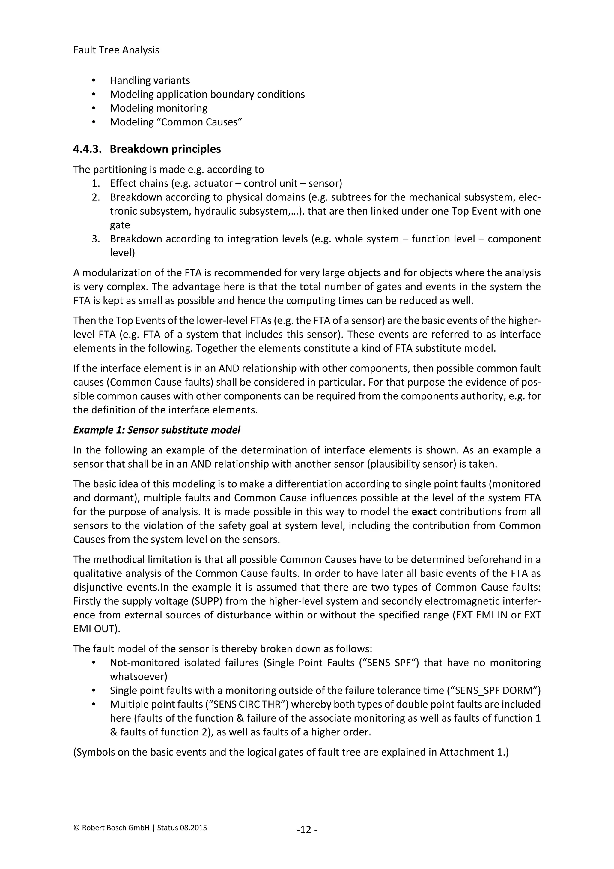
The document provides an overview of fault tree analysis (FTA):
- FTA is a deductive method used to identify causes of undesirable events and assess risks. It uses logic symbols in a tree structure to visually represent the relationships between failures.
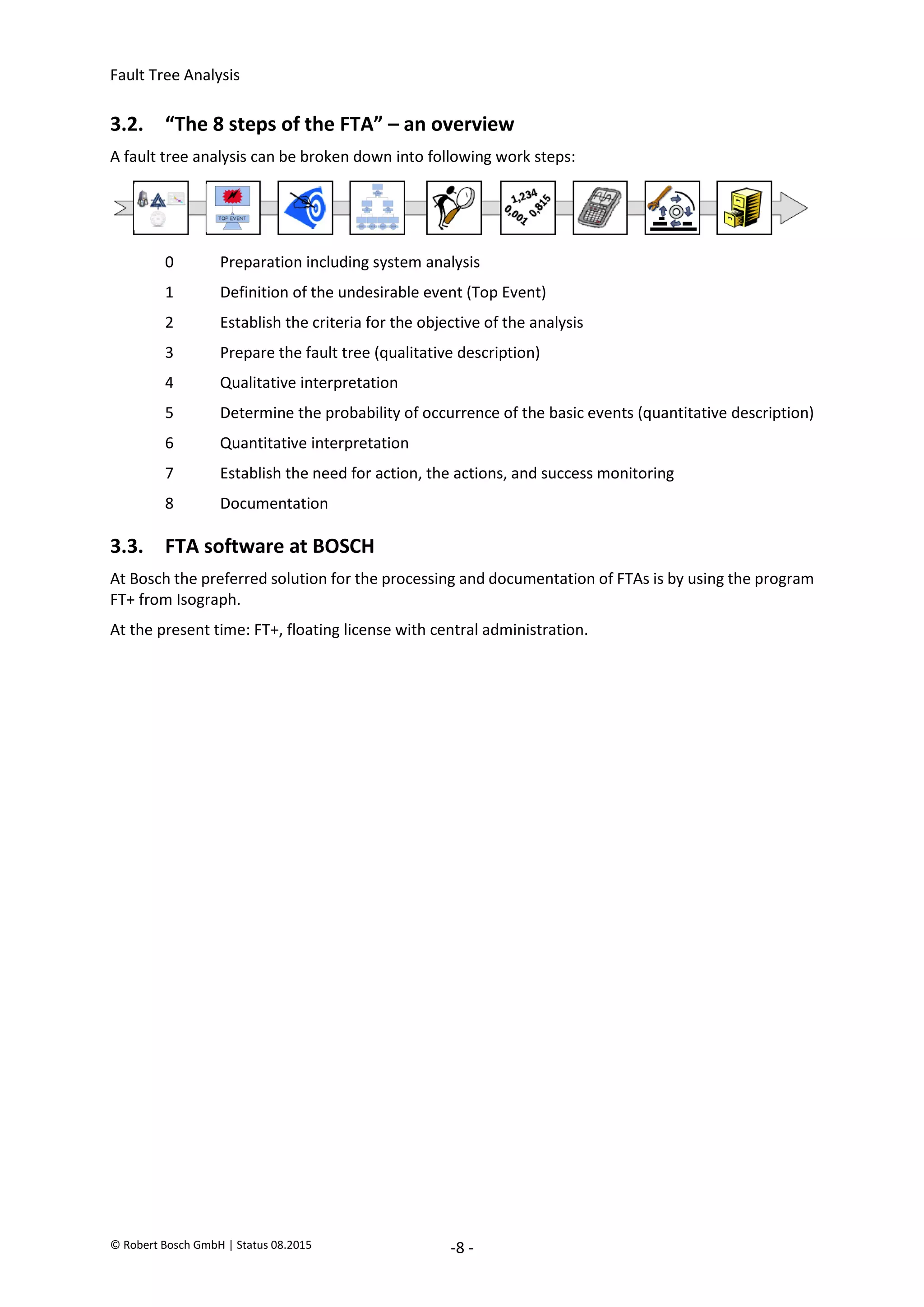
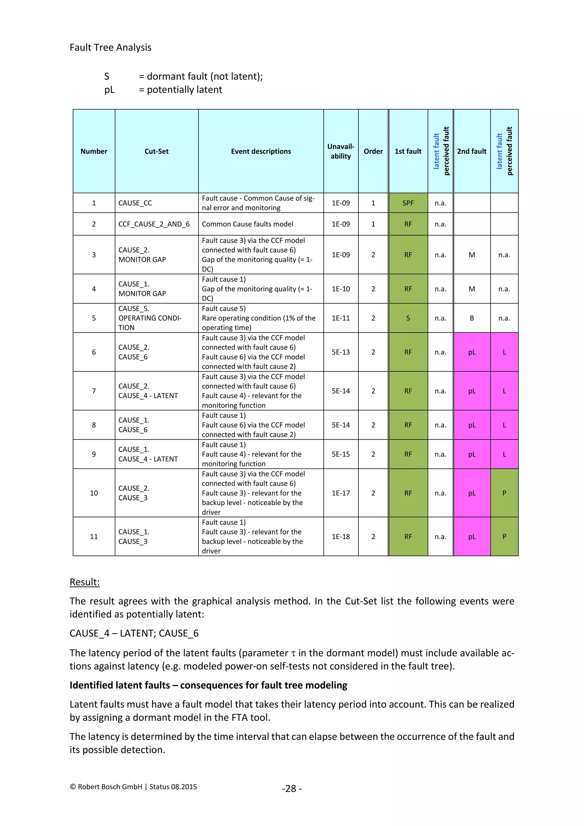
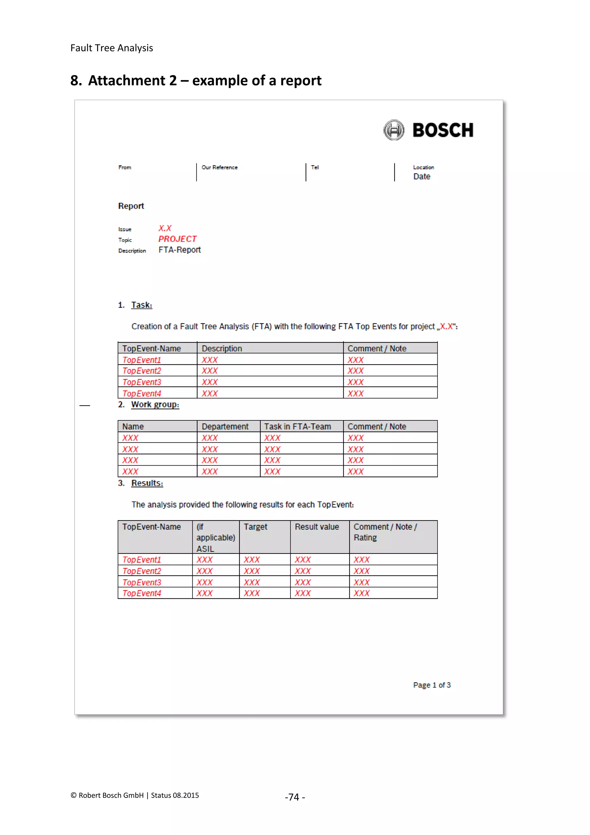
- The 8 key steps of FTA are defined as preparation, defining the undesirable event, establishing analysis criteria, constructing the fault tree, qualitative interpretation, determining failure probabilities, quantitative interpretation, and establishing corrective actions.
- FTA has benefits of systematically identifying failure causes and paths, allowing quantitative reliability analysis, and identifying improvement opportunities. Drawbacks include difficulty modeling dynamic systems and incomplete failure data limiting quantification.

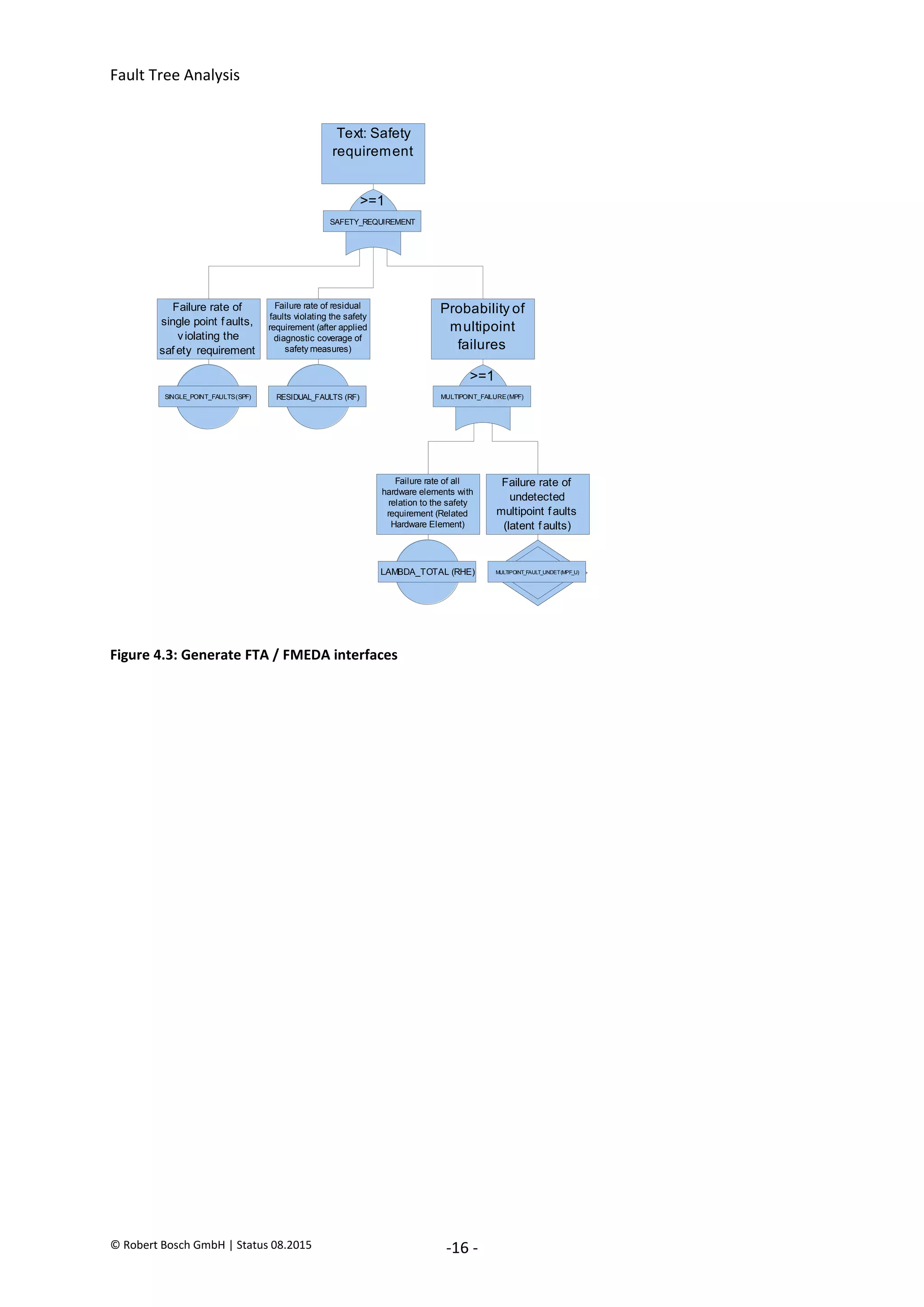
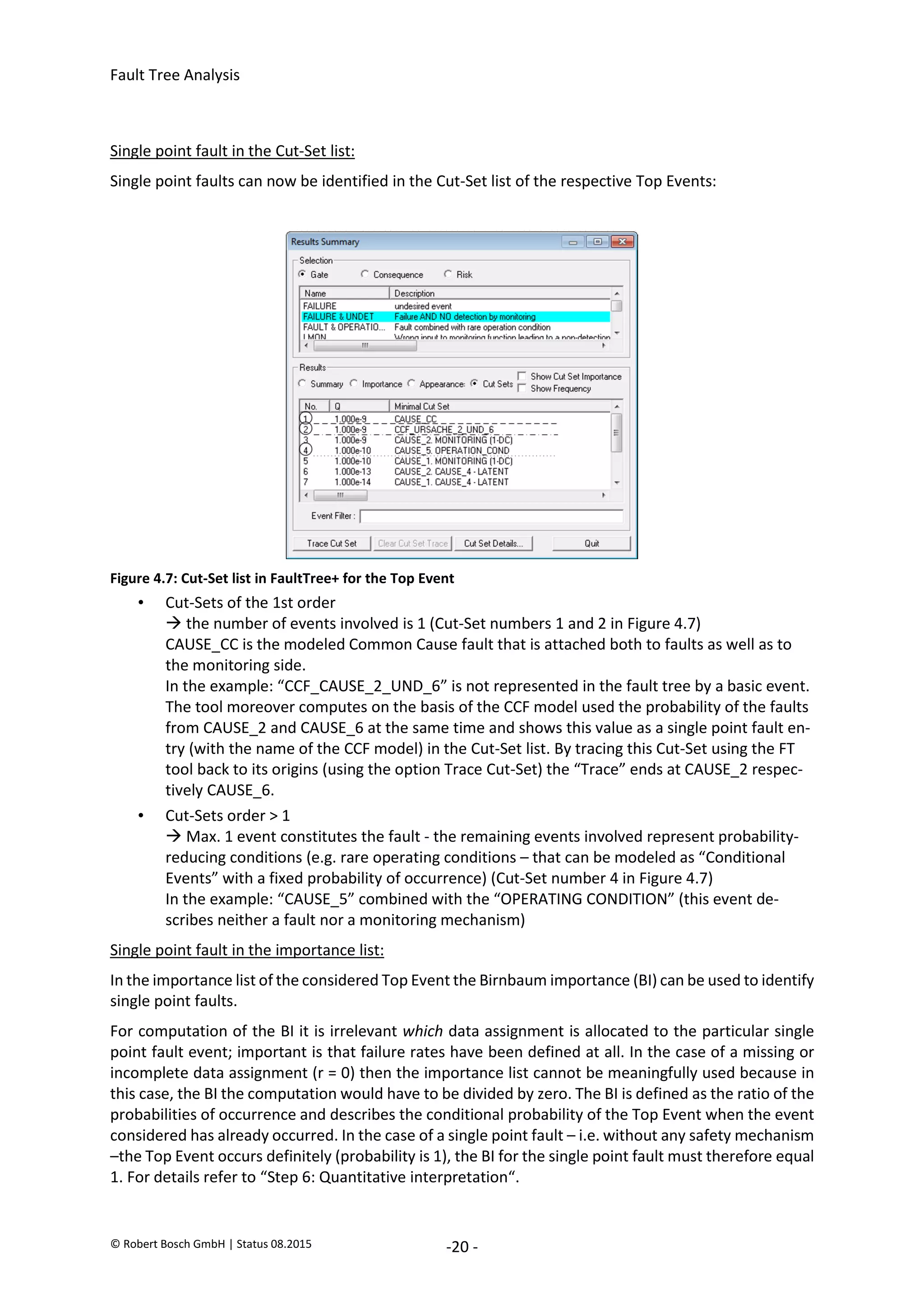
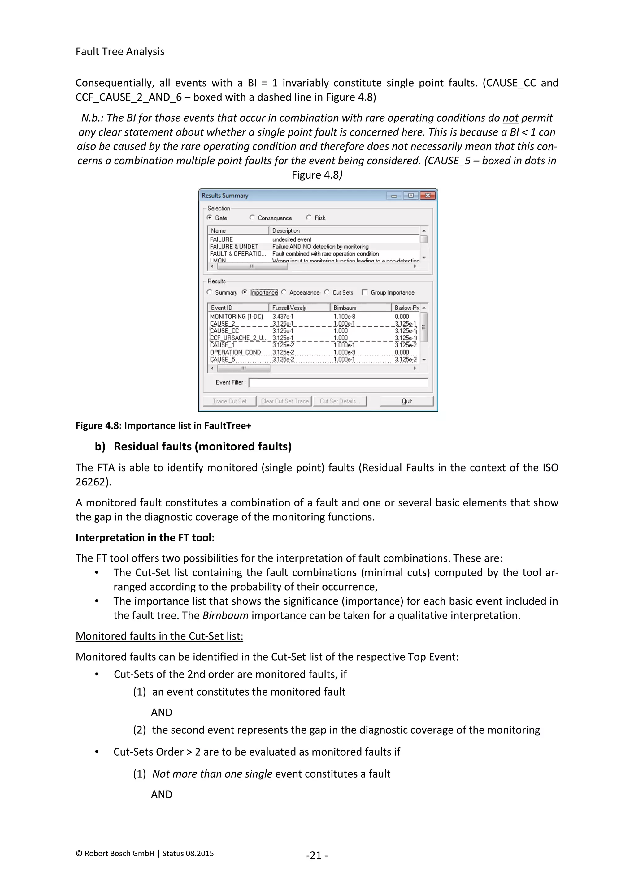
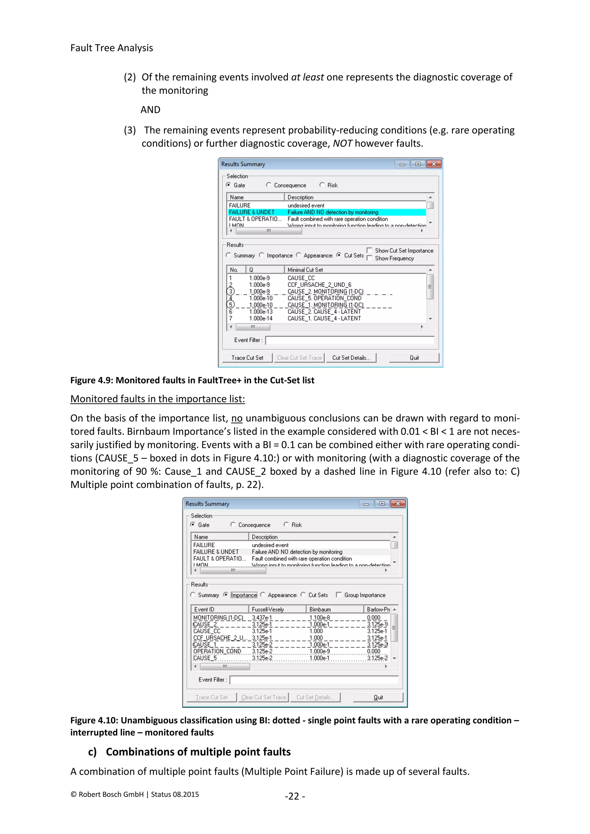
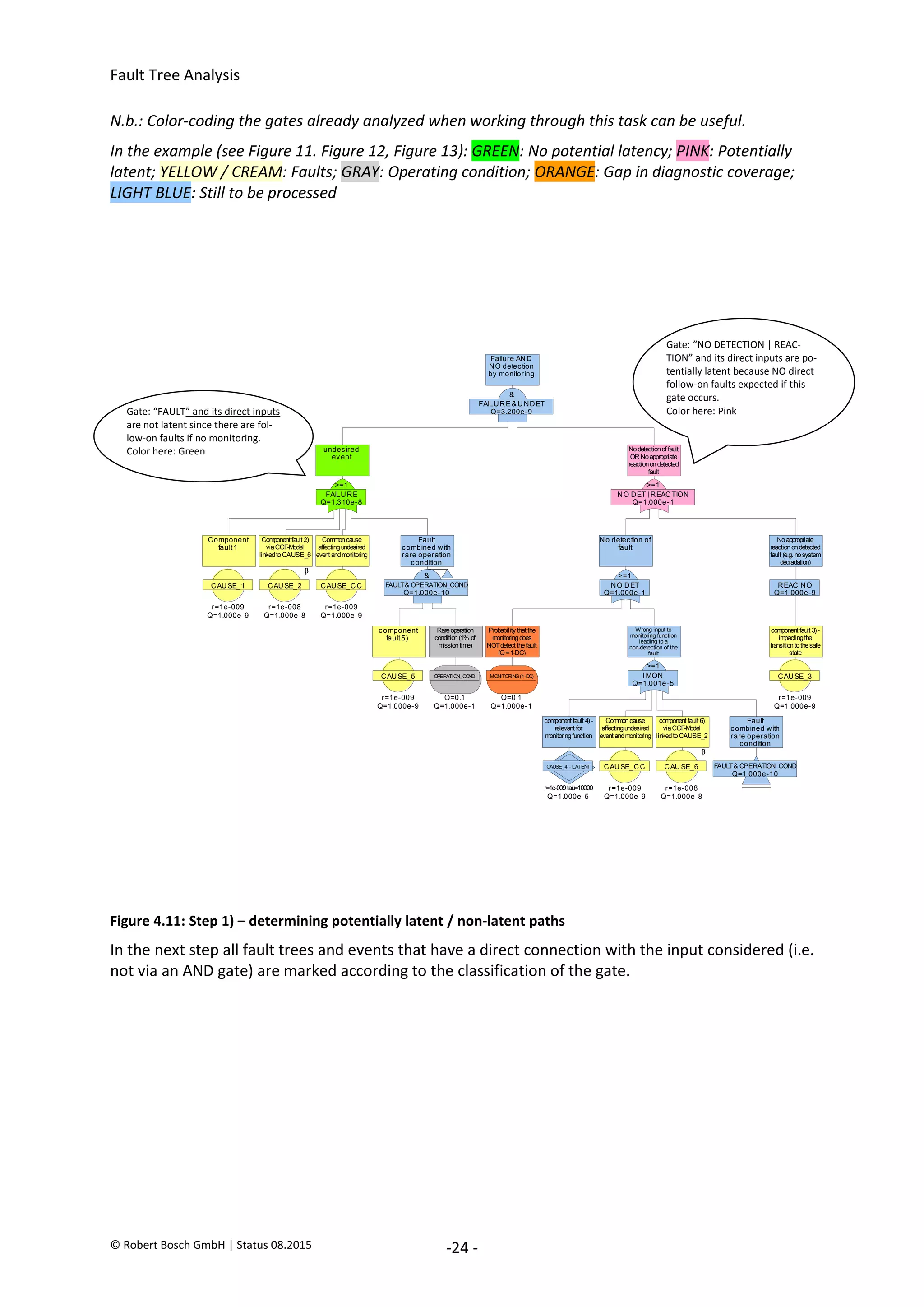

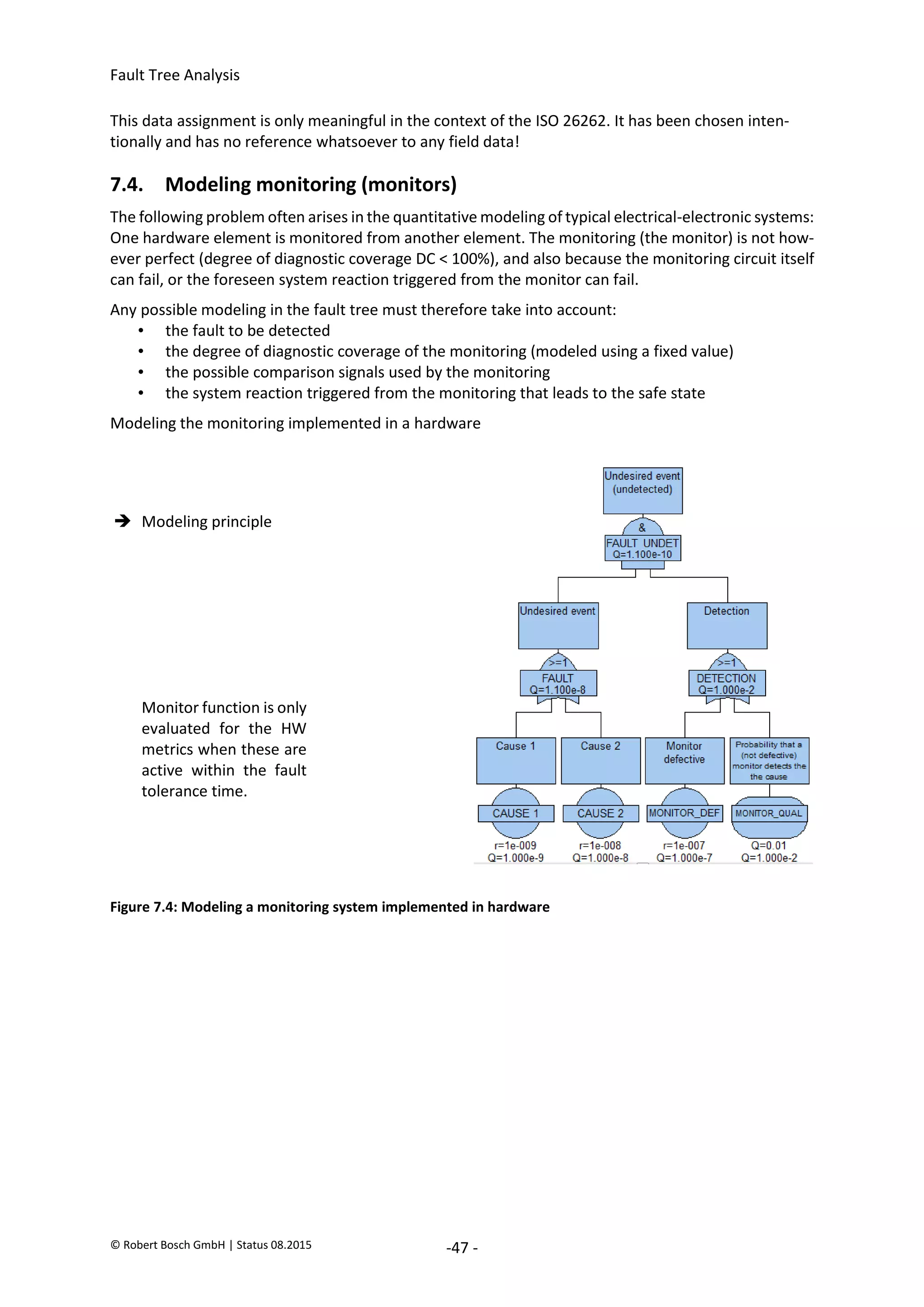
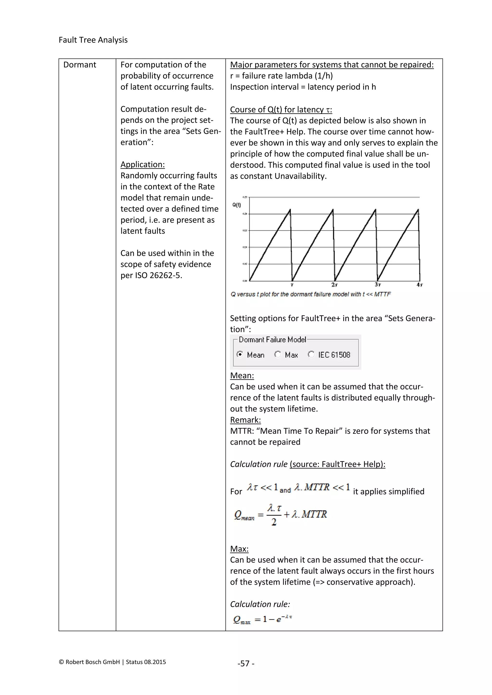
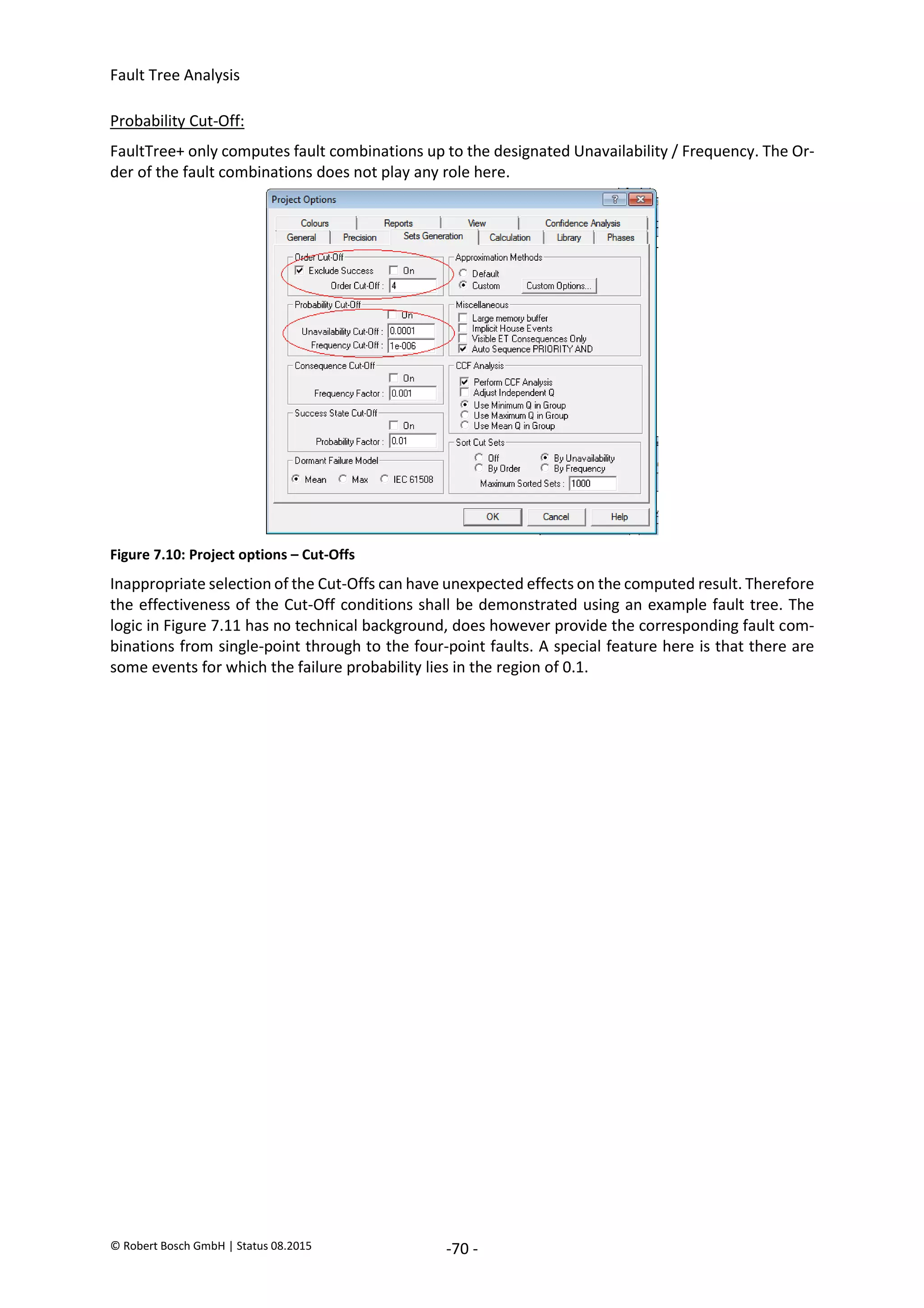
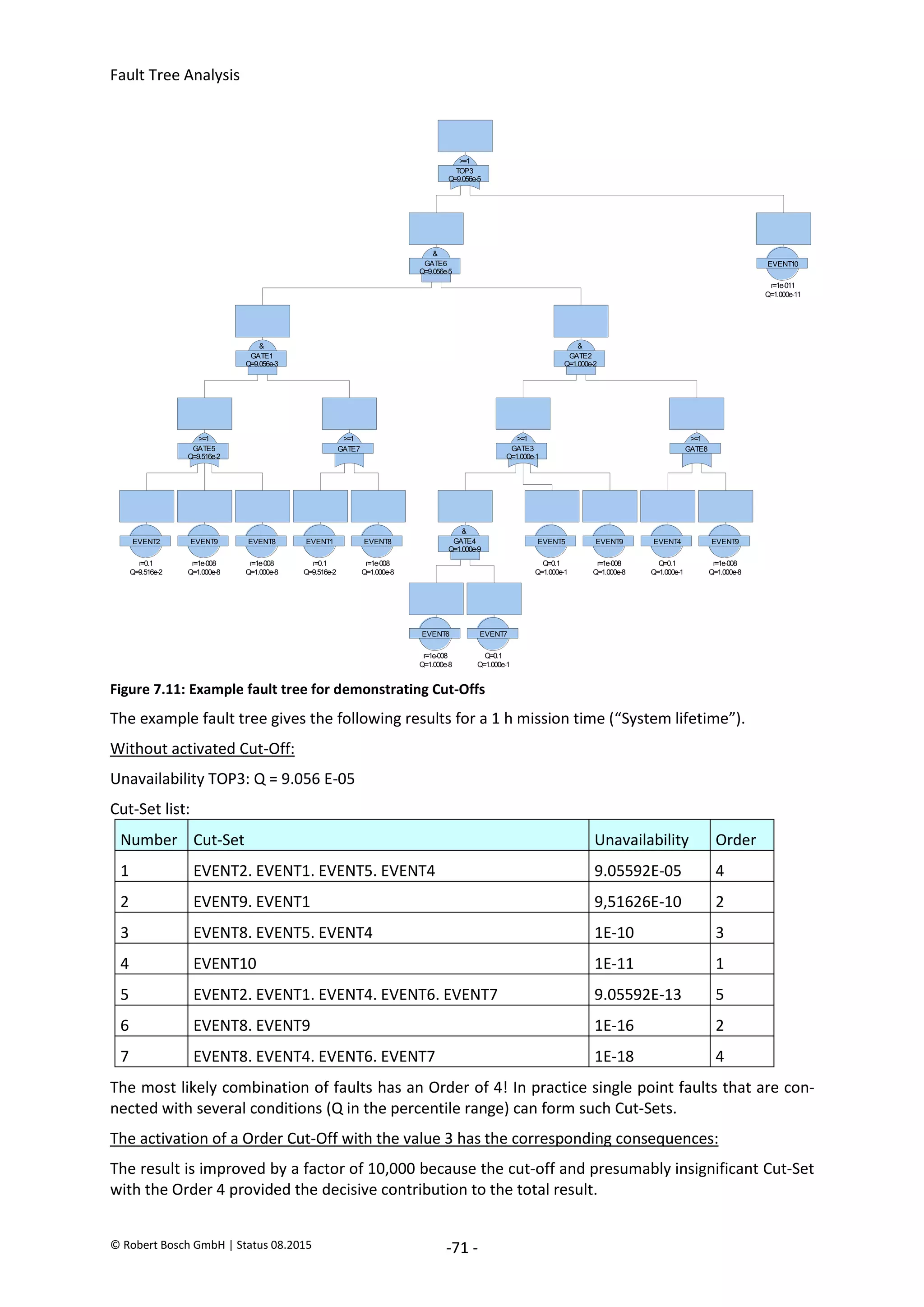
![Fault Tree Analysis
© Robert Bosch GmbH | Status 08.2015 -39 -
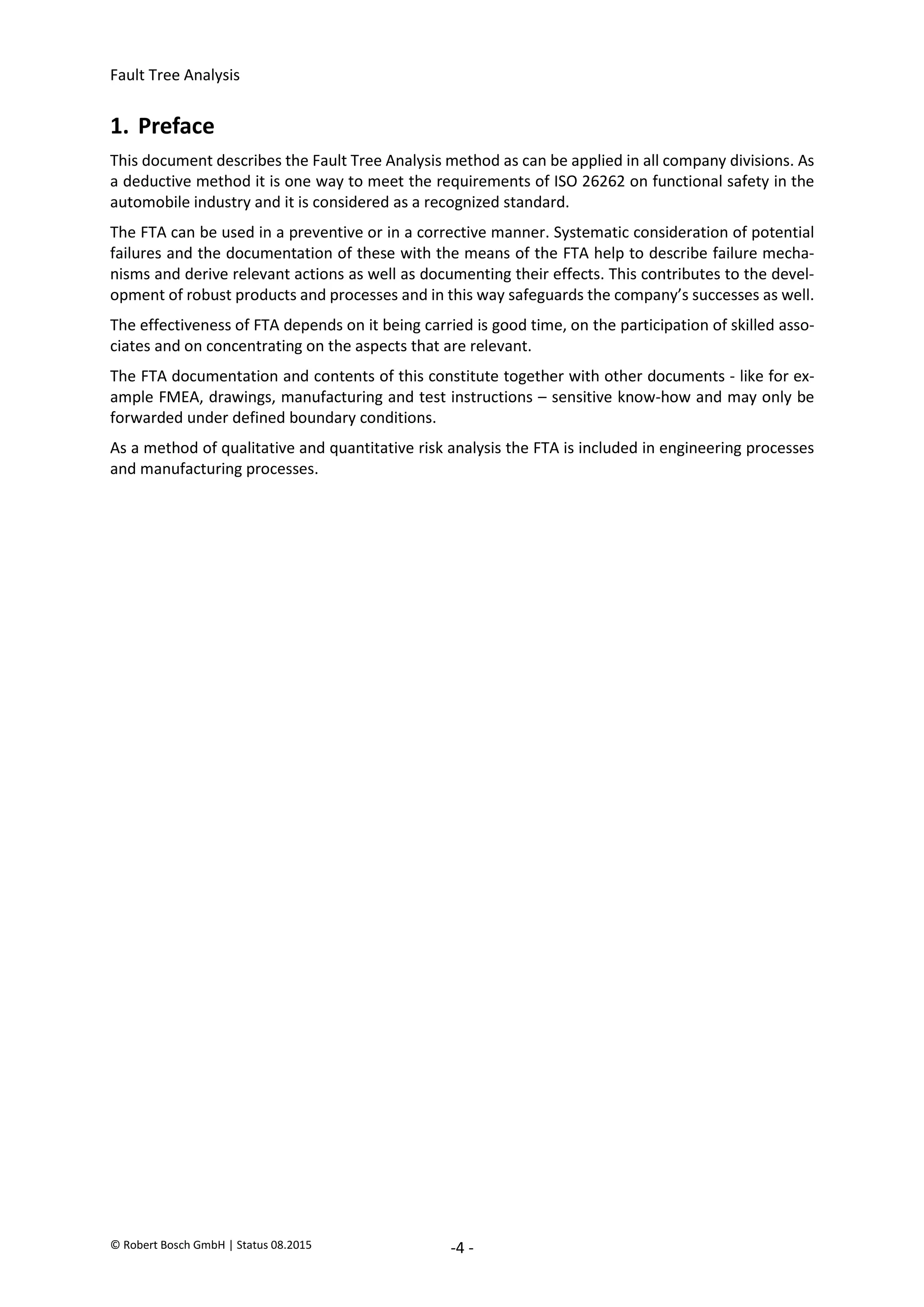
5. Literature on FTA
Norms, Guidelines, Handbooks
5.1. Norms
[5.1.1] DIN 25424-1, Fehlerbaumanalyse – Methode und Bildzeichen (Deutsche Norm)
Deutsches Institut für Normung, Sep. 1981, Beuth Verlag GmbH, Berlin
[5.1.2] DIN 25424-2, Fehlerbaumanalyse – Handrechenverfahren zur Auswertung eines Fehlerbau-
mes (Deutsche Norm)
Deutsches Institut für Normung, April 1990, Beuth Verlag GmbH, Berlin
[5.1.3] DIN EN 61025 Fehlzustandsbaumanalyse (Deutsche Version der europ. Norm EN 61025)
DKE Deutsche Kommission Elektrotechnik Elektronik Informationstechnik im DIN und VDE,
August 2007, Beuth Verlag GmbH, 10772 Berlin
[5.1.4] ISO 26262 Straßenfahrzeuge – Funktionale Sicherheit (Teil 1 - 10)
Internationale Organisation für Normung, November 2011, Genf (Schweiz)
[5.1.5] SN 29500, Ausfallraten Bauelemente (Teil 1-16) (Siemens Norm)
Siemens AG, 2004-2014, München und Erlangen
5.2. Standards
[5.2.1] Qualitätsmanagement in der Automobilindustrie, Band 4, Kapitel 4, Fehlerbaumanalyse
VDA, Verband der Automobilindustrie e.V., Oberursel, Deutschland (2003)
5.3. Handbooks
[5.3.1] Fault Tree Handbook, NUREG-0492 (US-Standard)
D. F. Haasl et al., U.S. Nuclear Regulatory Commission, Washington, USA (1981)
[5.3.2] Fault Tree Analysis Application Guide (international standard)
D. J. Mahar et al., Reliability Analysis Center, Rome, USA (1990)
[5.3.3] Fault Tree Handbook with Aerospace Applications (Aerospace industry)
W. Vesely et al., NASA Office of Safety and Mission Assurance, Washington, USA (2002)
[5.3.4] VDI 4008 Blatt 7, Strukturfunktion und ihre Anwendung (VDI-Handbuch Technische Zuver-
lässigkeit)
Verein Deutscher Ingenieure, VDI-Verlag GmbH, Düsseldorf (1986), Bezug: Beuth Verlag GmbH, Berlin
[5.3.5] IEC TR 62380, Reliability Data Handbook (Internationaler Standard)
(Ermittlung von Zuverlässigkeitsdaten, the für the Berechnung der FTA benötigt werden)
Internat. Electrotechnical Commission, Geneve, Switzerland (2004)
[5.3.6] Reliability Engineering: Theory and Practice
Alessandro Birolini, ISBN: 3-642-39534-1, Springer Verlag, 2014 (7th edition)
2020-04-06
-
SOCOS
•••••••••
•••••••••](https://image.slidesharecdn.com/faulttreeanalysis-230702025029-121e1627/75/Fault-Tree-Analysis-pdf-41-2048.jpg)
![Fault Tree Analysis
© Robert Bosch GmbH | Status 08.2015 -40 -
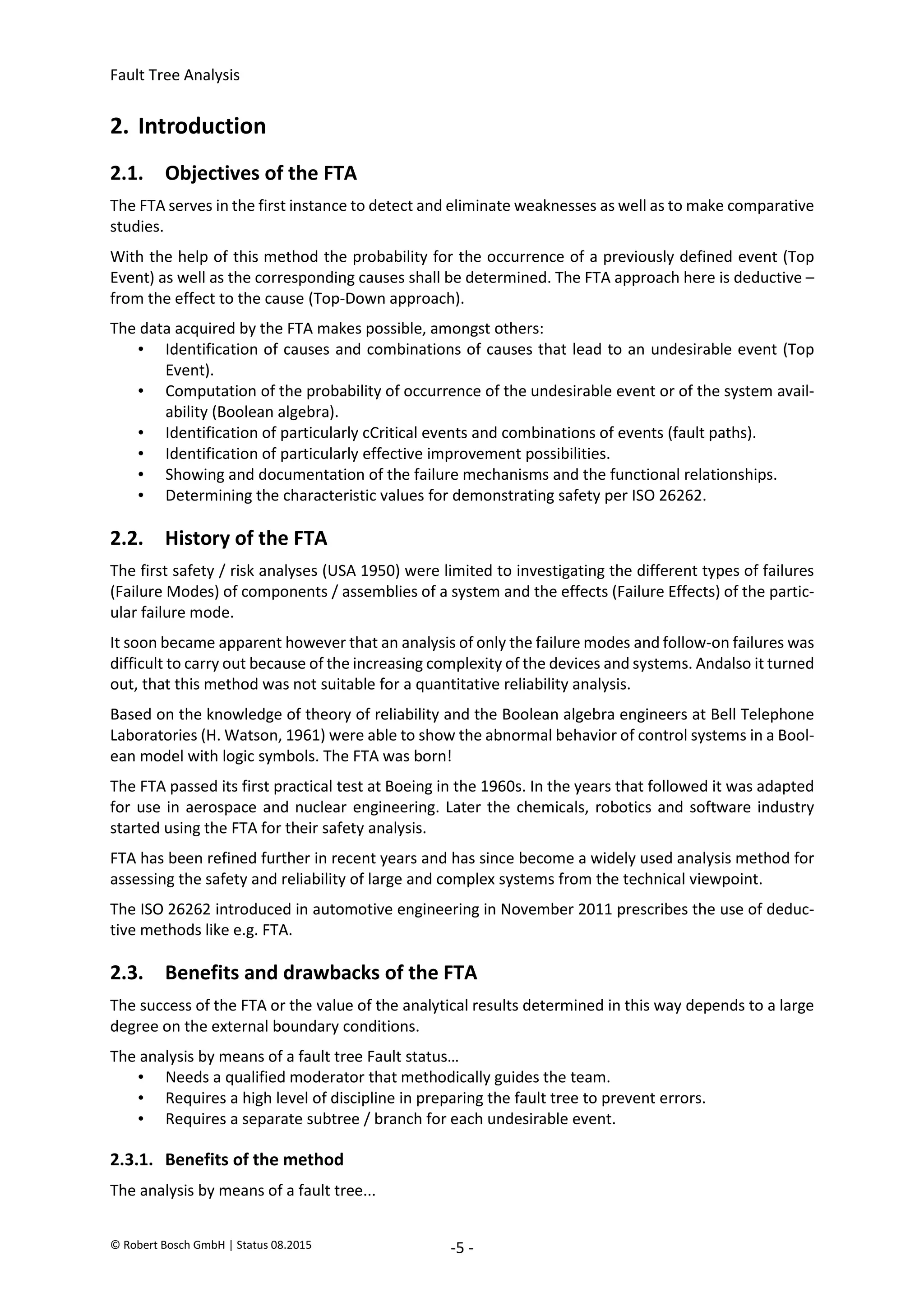
5.4. Reference books
[5.4.1] Die Fehlerbaum-Methode
W. Schneeweiss, ISBN 3-934447-02-3, LiLoLe Verlag, Hagen, Germany (1999)
[5.4.2] Taschenbuch der Zuverlässigkeits- und Sicherheitstechnik
(Darstellung unterschiedlicher Methothe und Techniken der Zuverlässigkeits- und Sicherheitstechnik)
A. Meyna, B. Pauli et al., ISBN 3-446-21594-8, Carl Hanser Verlag, München – Wien (2003)
[5.4.3] Fault Tree Analysis Primer
Clifton A. Ericson II, ISBN 9781466446106, CreateSpace Inc., Charleston, NC (2011)
[5.4.4] Fehlerbaumanalyse in Theorie und Praxis
(Grundlagen und Anwendung der Methode), F. Edler, M. Soden, R. Hankammer
ISBN 9783662481653, Springer-Verlag, Berlin Heidelberg (2015)
[5.4.5] Erstellung von Fehlerbäumen
(Eine strukturierte und systematische Methode), W. Freese, ISBN 9783446445161,
Carl Hanser Verlag, München (2015)
2020-04-06
-
SOCOS
•••••••••
•••••••••](https://image.slidesharecdn.com/faulttreeanalysis-230702025029-121e1627/75/Fault-Tree-Analysis-pdf-42-2048.jpg)
![Fault Tree Analysis
© Robert Bosch GmbH | Status 08.2015 -52 -
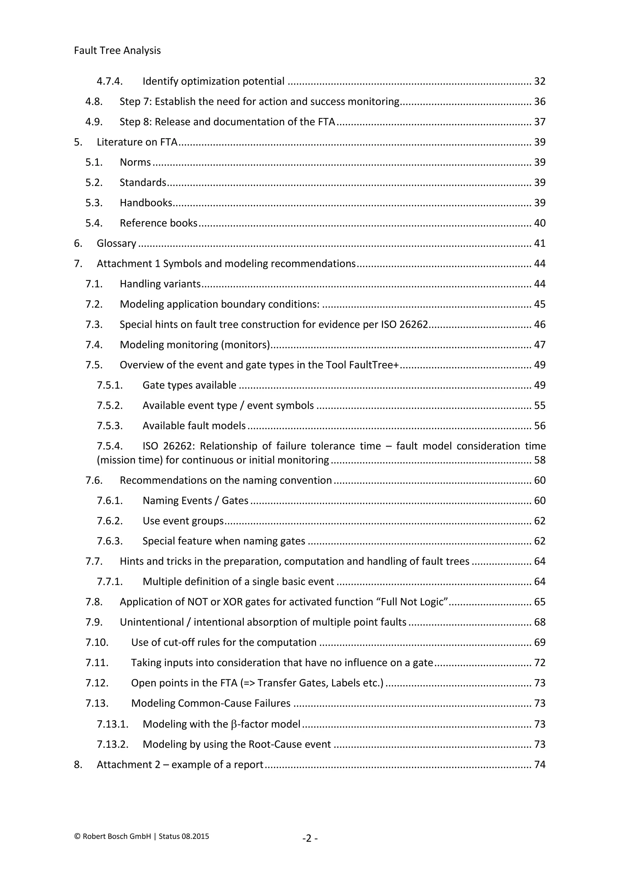
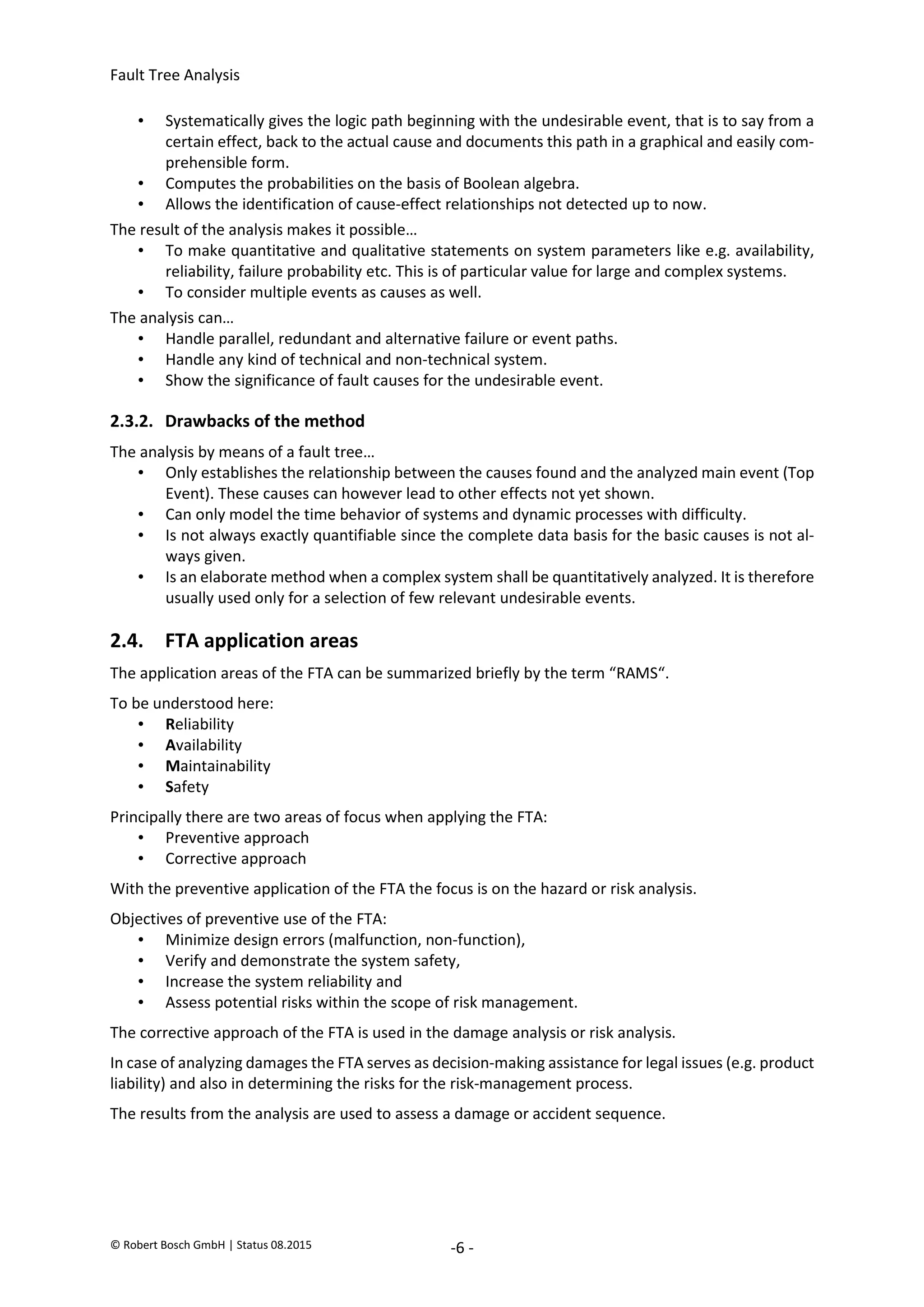
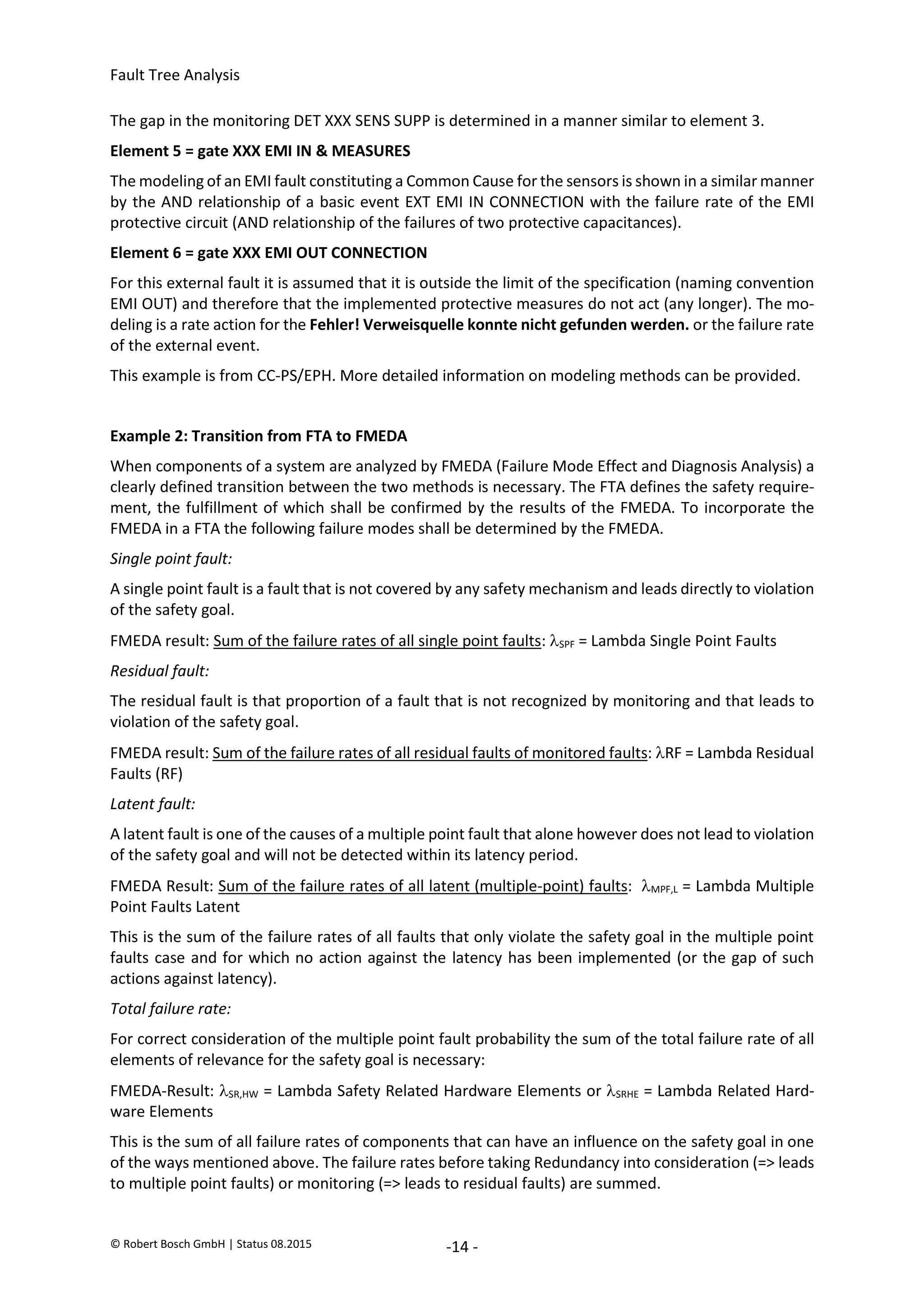
Type Symbol Remark
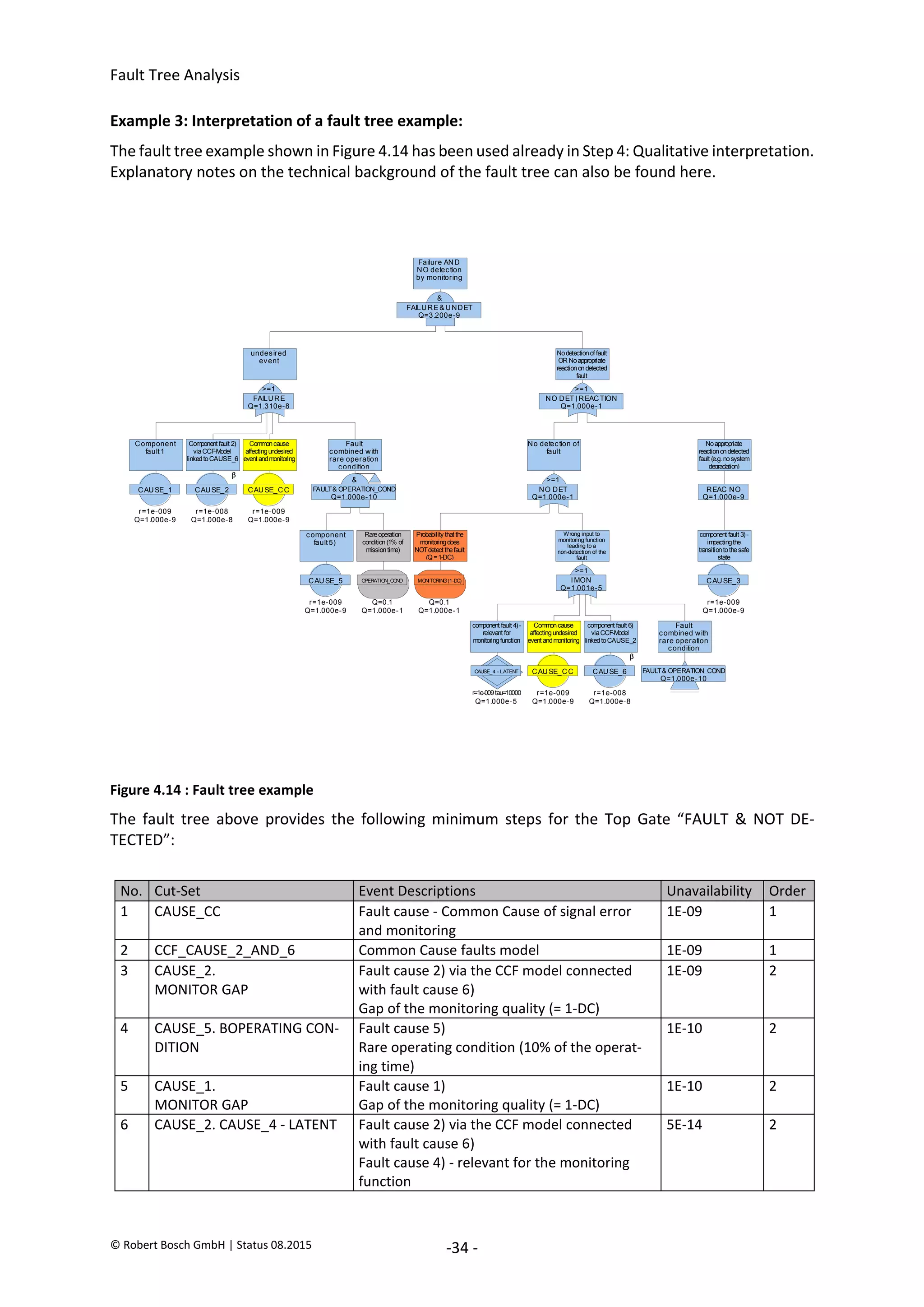
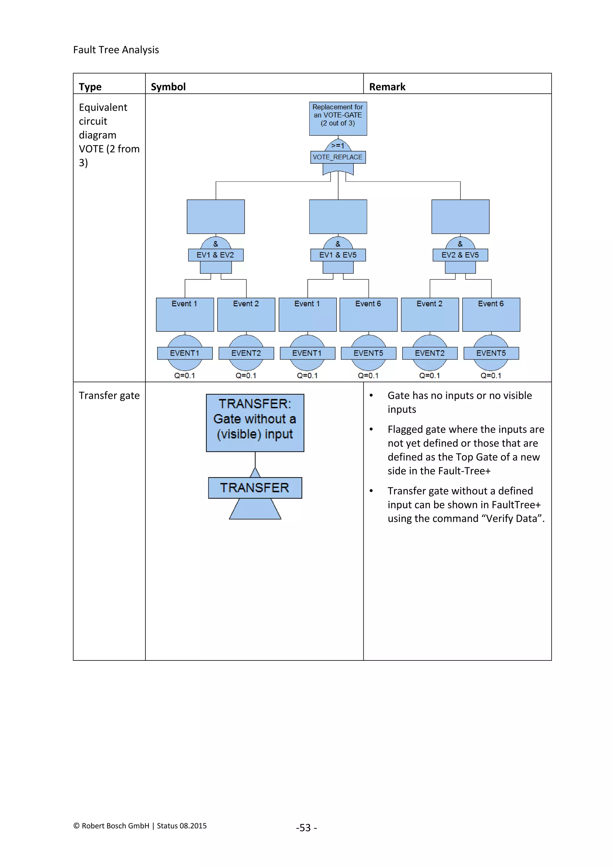
Vote gate (n
from m)
Remark:
• n from m inputs must be TRUE.
Here: 2 from 3 inputs...
• (AB)(AC)(BC)
• Cut-Set list:
EVENT1.EVENT2
EVENT1.EVENT6
EVENT2.EVENT6
• Computation of Q (summation rule)
Q = qA*qB + qA*qC + qB*qC
- [(qA*qB)*(qA*qC) + (qA*qB)*(qB*qC) + (qB*qC)*(qA*qC)]
+ (qA*qB)*(qA*qC)*(qB*qC)
= qA*qB + qA*qC + qB*qC - [(qA*qB*qC) + (qA*qB*qC) + (qB*qC*qA)]
+ (qA*qB*qC)
• In the example the following applies...
qx*qy = 0.01
qx*qy*qz = 0.001
• Also:
Q = 0.01 + 0.01 + 0.01 - [0.001 + 0.001 + 0.001] + 0.001
= 0.03 – 0.003 + 0.001
= 0.028
• Remark: FaultTree+ limits the maximum number of inputs to 18
2020-04-06
-
SOCOS
•••••••••
•••••••••](https://image.slidesharecdn.com/faulttreeanalysis-230702025029-121e1627/75/Fault-Tree-Analysis-pdf-54-2048.jpg)

![Fault Tree Analysis
© Robert Bosch GmbH | Status 08.2015 -62 -
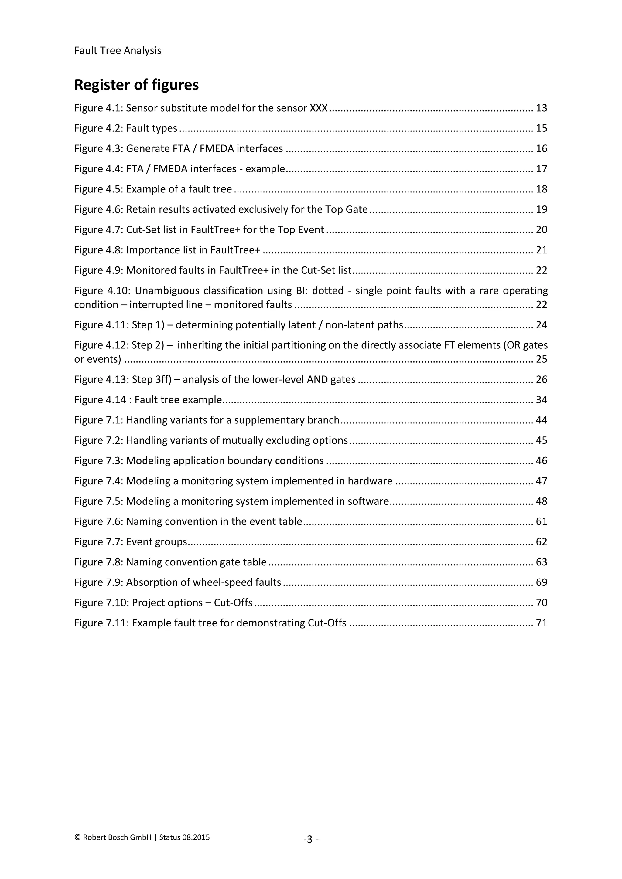
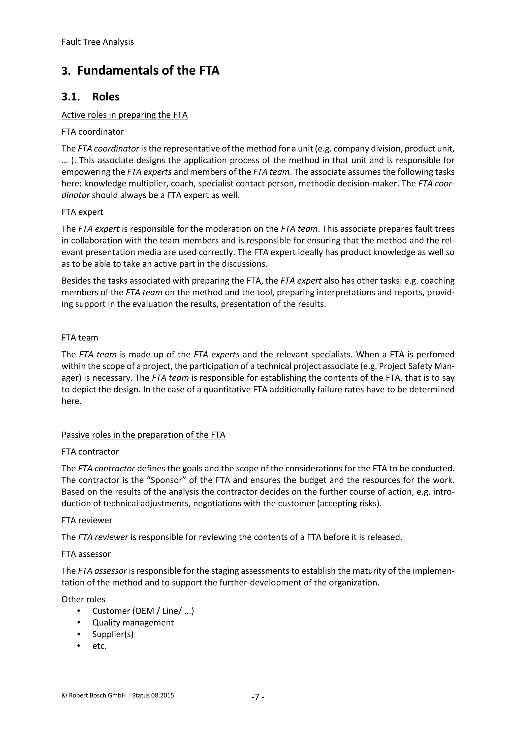
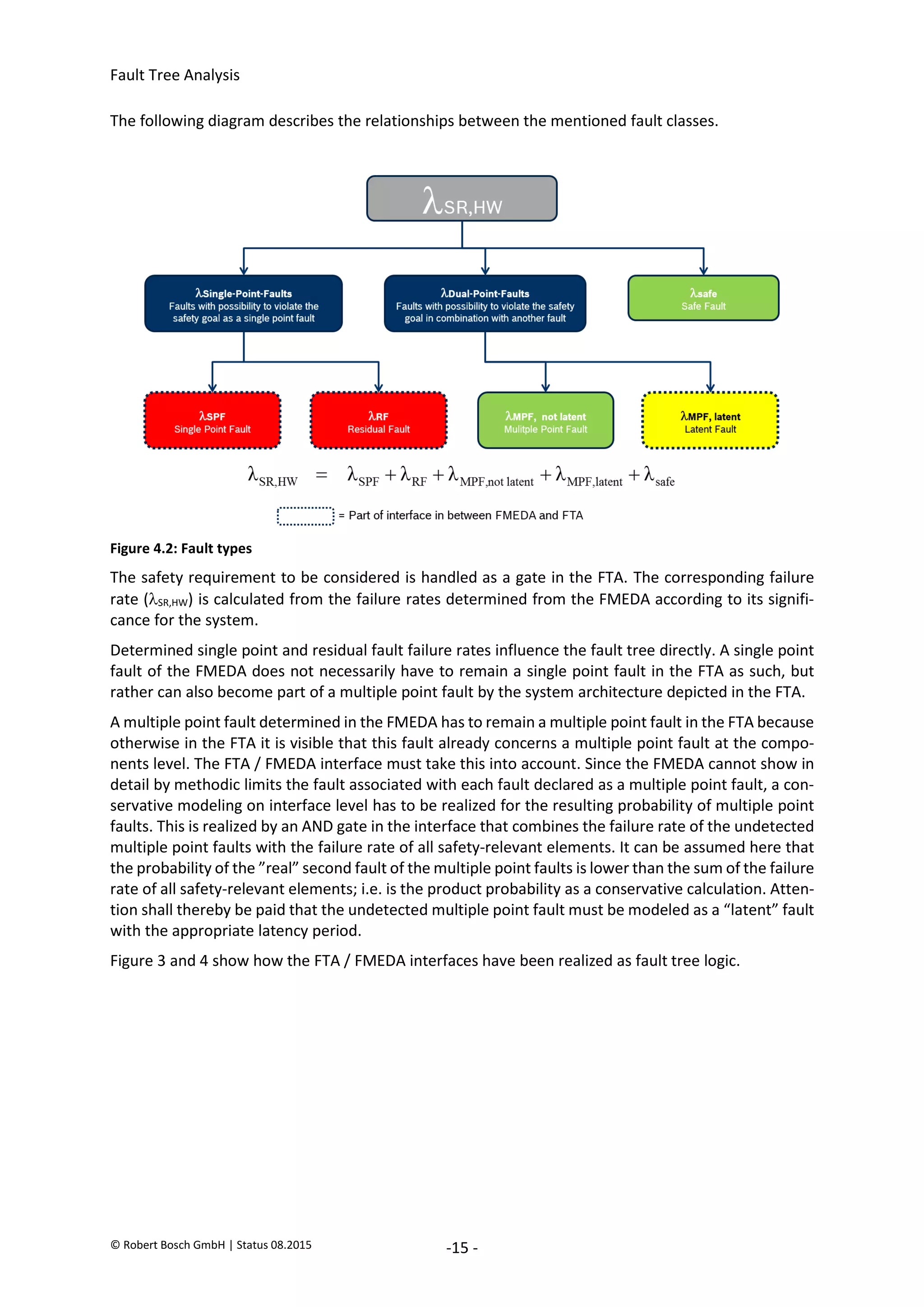
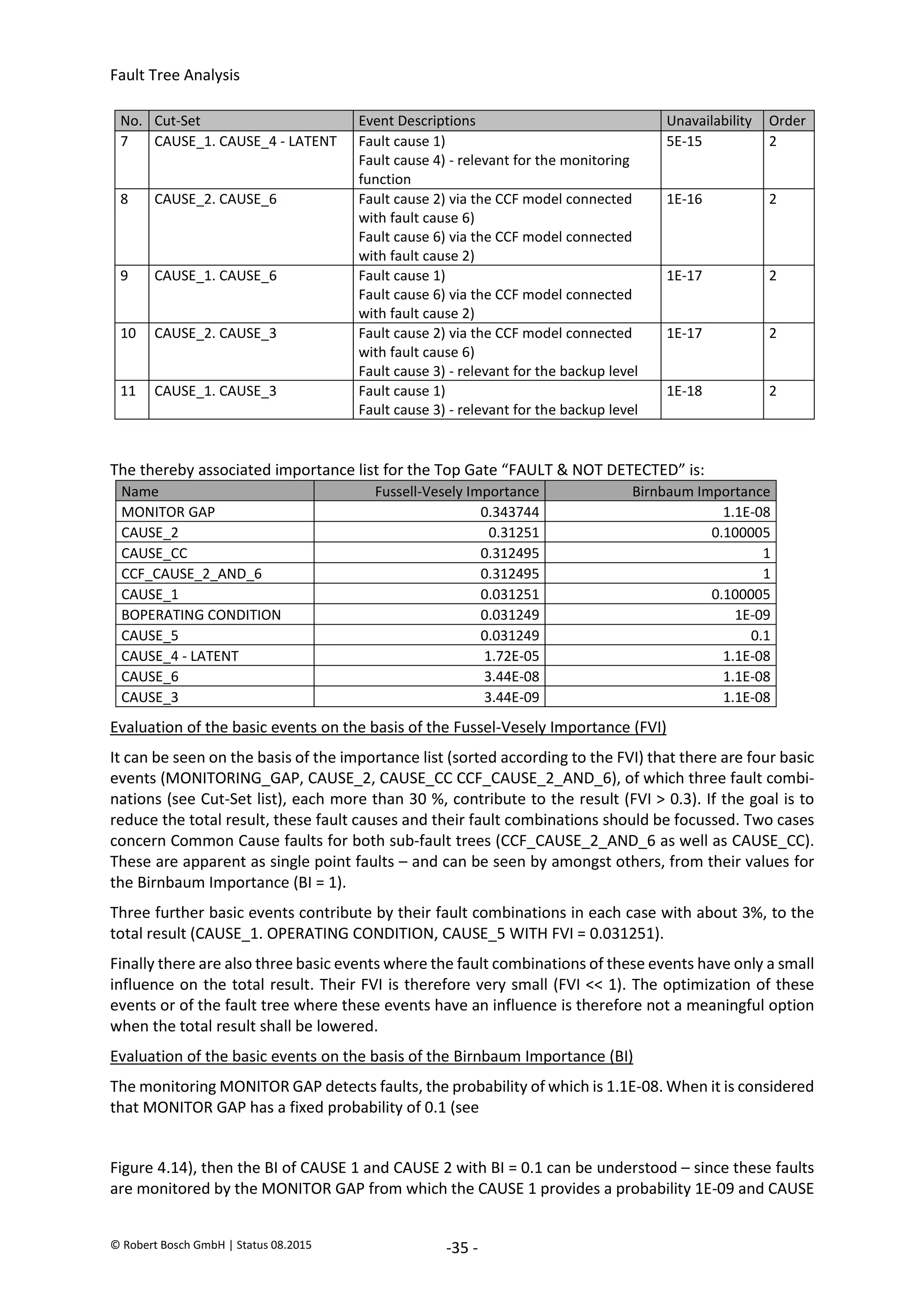
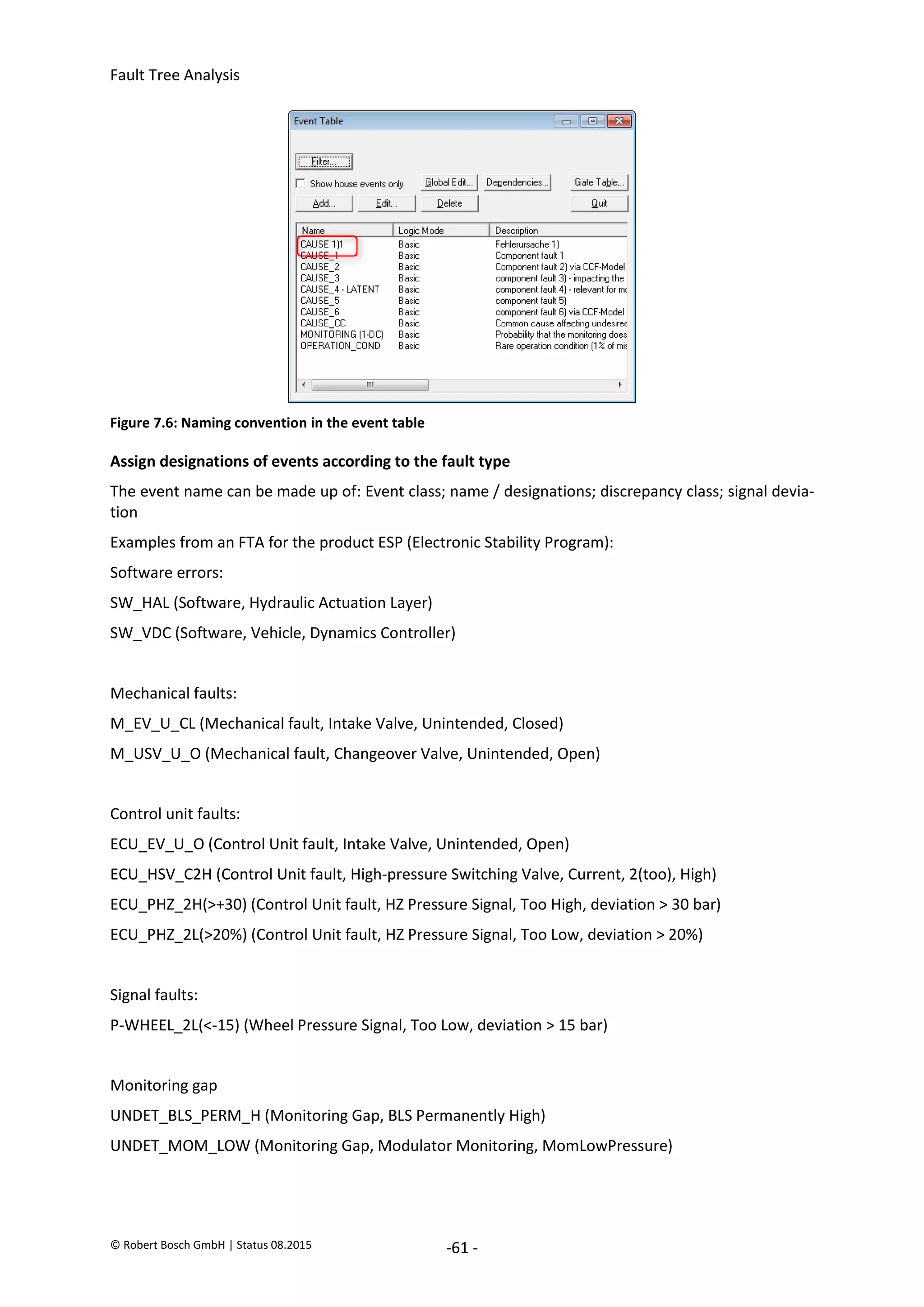
7.6.2. Use event groups
If the number of assigned events increases, then sorting the events into groups can help to retain the
overview. Event groups are created in FaultTree+ in the project Explorer. Assigning an event to several
event groups is also possible.
Figure 7.7: Event groups
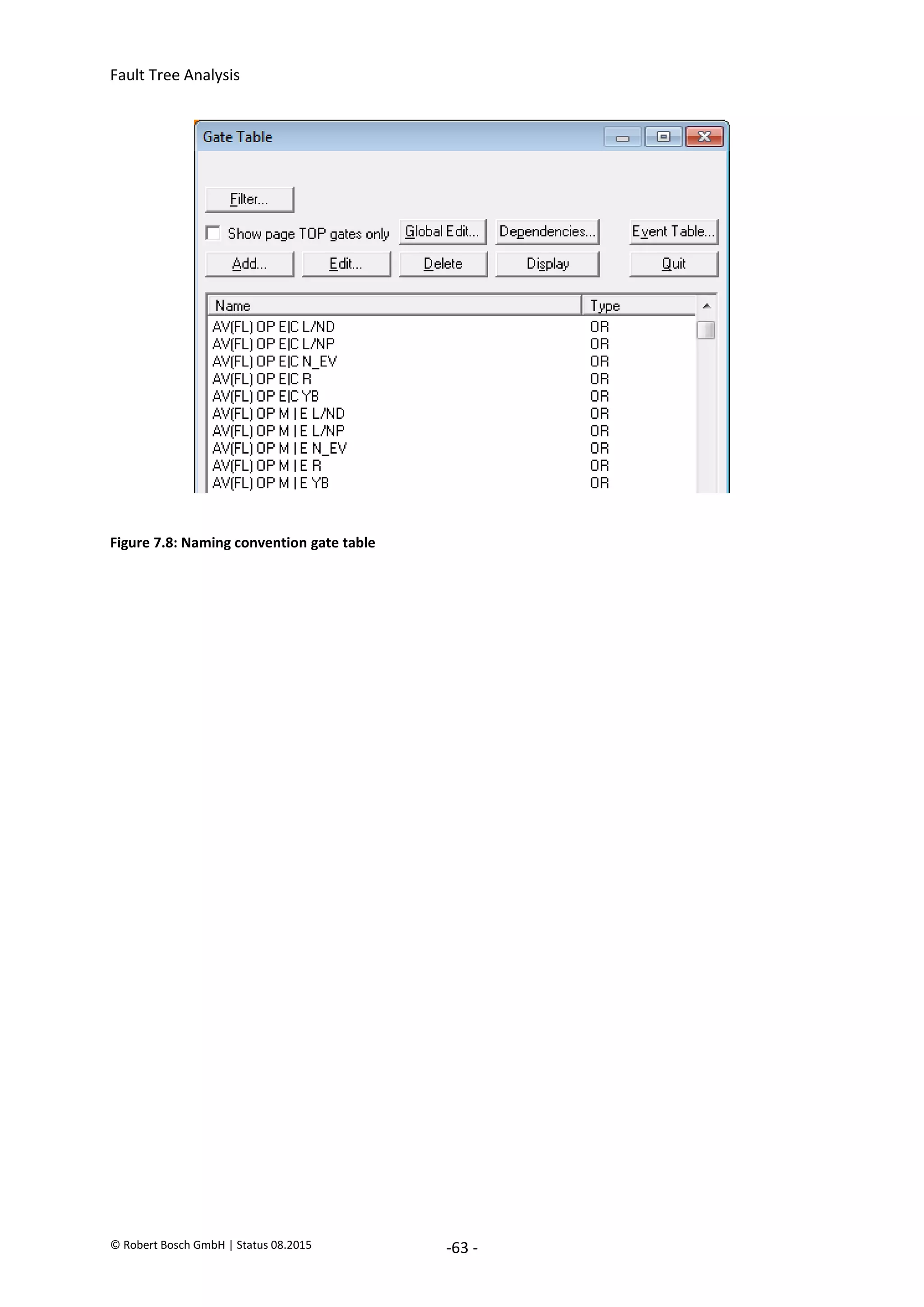
7.6.3. Special feature when naming gates
If a file contains several sub-fault trees that analyze the different Top Events, then it can be meaningful
when the designations of the gates include indications about the inclusion in the particular sub-fault
tree. If the note is added at the end of the designation then this has the advantage that similar gates
which are sorted alphabetically are listed side-by-side by FaultTree+ in different hazards.
Advantage: Especially the relationships between the gates are easier to understand. Contradictions
(repeatedly used) signal-fault trees and the Top Event (the Hazard) of the fault tree can be (more)
easily identified.
Example for the identification of gates within fault trees (last letters):
AV(FL) OP E|C * [Exhaust Valve] [(Wheel Front Left)] [Open] [Electrical or Control fault] [identifica-
tion for the respective fault tree (L/ND, L/NP, R,...)]
AV(FL) OP M|E * [Exhaust Valve] [(Wheel Front Left)] [Open] [Mechanical or Electrical fault] [iden-
tification for the respective fault tree (L/ND, L/NP, R, ...)]
2020-04-06
-
SOCOS
•••••••••
•••••••••](https://image.slidesharecdn.com/faulttreeanalysis-230702025029-121e1627/75/Fault-Tree-Analysis-pdf-64-2048.jpg)


![[SiriusCon 2020] Realization of Model-Based Safety Analysis and Integration w...](https://cdn.slidesharecdn.com/ss_thumbnails/siriusconslidesfinalslidesmzellersiemens-200624092330-thumbnail.jpg?width=640&height=640&fit=bounds)


![[DSC Europe 25] Debmalya Biswas - Agentification: the art of transforming man...](https://cdn.slidesharecdn.com/ss_thumbnails/r5azlggvtqiaiiusrqdr-4-251212103249-5a12c89b-thumbnail.jpg?width=640&height=640&fit=bounds)
![[DSC Europe 25] Tatevik Maytesyan - How to actually use AI in marketing: gett...](https://cdn.slidesharecdn.com/ss_thumbnails/tjo626lsqdgfntbgl2mw-4-251216103155-e36cd239-thumbnail.jpg?width=640&height=640&fit=bounds)


![[DSC Europe 25] Hans Kleinsman - The Compliance Gearbox: How Tax Tech Mediate...](https://cdn.slidesharecdn.com/ss_thumbnails/dxdytie1toel0hr90bjs-2-251212103250-174fdbe7-thumbnail.jpg?width=640&height=640&fit=bounds)
![[DSC Europe 25] Jon Dajci - Bridging TradFi and DeFi: Building the Future of ...](https://cdn.slidesharecdn.com/ss_thumbnails/fqmhfvlbqhkihjvqvhmu-7-251211083849-6af7e325-thumbnail.jpg?width=640&height=640&fit=bounds)
![[DSC Europe 25] Danica Soc - The Science Behind Marketing: Experimentation me...](https://cdn.slidesharecdn.com/ss_thumbnails/c0nofsggs9gw5ucmallr-3-251216103155-56bd64d1-thumbnail.jpg?width=640&height=640&fit=bounds)
![[DSC Europe 25] Dusan Nesic - Securing Tomorrow’s Infrastructure: Why Cyber-P...](https://cdn.slidesharecdn.com/ss_thumbnails/qikbszfftyowjm2q6duw-1-251211083848-8f2ead6b-thumbnail.jpg?width=640&height=640&fit=bounds)
![[DSC Europe 25] Bassam Maharmeh - Artificial Intelligence: Opportunities and ...](https://cdn.slidesharecdn.com/ss_thumbnails/thhfmr2fqpawzj7hsjpg-5-251211083048-2c23204f-thumbnail.jpg?width=640&height=640&fit=bounds)


![[DSC Europe 25] Branko Dzakula - From Defense to Attack: How AI Redefines Cyb...](https://cdn.slidesharecdn.com/ss_thumbnails/80bdzdxpr3ky2g0qvyk9-8-251211083048-ce5fc1ee-thumbnail.jpg?width=640&height=640&fit=bounds)
