This document summarizes research on deep learning approaches for face recognition. It describes the DeepFace model from Facebook, which used a deep convolutional network trained on 4.4 million faces to achieve state-of-the-art accuracy on the Labeled Faces in the Wild (LFW) dataset. It also summarizes the DeepID2 and DeepID3 models from Chinese University of Hong Kong, which employed joint identification-verification training of convolutional networks and achieved performance comparable or superior to DeepFace on LFW. Evaluation metrics for face verification and identification tasks are also outlined.


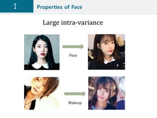

![Properties of Face
Diverse Recognition Scenes
Adopted from [8].](https://image.slidesharecdn.com/facerecognitionv1-190528022819/85/Face-recognition-v1-5-320.jpg)
![Properties of Face
Prior: face images lie on a manifold [15-17]
Adopted from [15]](https://image.slidesharecdn.com/facerecognitionv1-190528022819/85/Face-recognition-v1-6-320.jpg)
![Holistic learning
Eigenfaces [1][2]
Adopted from Wikipedia(Eigenface)
Fisherfaces [2]
Adopted from OpenCV Docs.(Face Recognition)
Bayes, Laplacianface 2DPCA, SRC, CRC, Metric Learning, etc.](https://image.slidesharecdn.com/facerecognitionv1-190528022819/85/Face-recognition-v1-7-320.jpg)
![Local handcraft
Gabor filter [3]
Adopted from Mathworks.com
(Gabor Feature Extraction)
Local Binary Pattern [4][5][6]
Adopted from Scikit-image (Local Binary Pattern for texture classification).
EBGM, LGBP, HD-LBP, etc.](https://image.slidesharecdn.com/facerecognitionv1-190528022819/85/Face-recognition-v1-8-320.jpg)
![Deep learning
DeepFace (Facebook, CVPR 2014)[7]
Adopted from [7].](https://image.slidesharecdn.com/facerecognitionv1-190528022819/85/Face-recognition-v1-9-320.jpg)
![Training, evaluation protocol
Training protocol,
Evaluation protocol
Adopted from [9].](https://image.slidesharecdn.com/facerecognitionv1-190528022819/85/Face-recognition-v1-10-320.jpg)
![Training, evaluation protocol
Training, Evaluation protocol
Adopted from [8].](https://image.slidesharecdn.com/facerecognitionv1-190528022819/85/Face-recognition-v1-11-320.jpg)
![Training, evaluation protocol
Training, Evaluation protocol
Adopted from [8].](https://image.slidesharecdn.com/facerecognitionv1-190528022819/85/Face-recognition-v1-12-320.jpg)

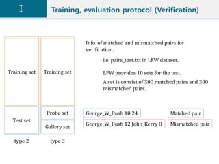
![Training, evaluation protocol (Verification)
Training, Evaluation protocol for LFW dataset
Adopted from [11].
1. Unrestricted, Labeled Outside Data
2. Unrestricted, No Outside Data
Commonly,](https://image.slidesharecdn.com/facerecognitionv1-190528022819/85/Face-recognition-v1-15-320.jpg)
![Training, evaluation protocol (Identification)
Training set
Probe set
Gallery set
type 3
Training set
Probe set
Gallery set
type 4
Close-set Identification Adopted from [8].
Open-set Identification Adopted from [8].](https://image.slidesharecdn.com/facerecognitionv1-190528022819/85/Face-recognition-v1-16-320.jpg)
![Dataset
Long tail distribution
Adopted from [8].
• The depth of dataset enforces the trained model to address a wide range
intra-class variations, such as lighting, age, and pose.
• The breadth of dataset ensures the trained model to cover the sufficiently
variable appearance of various people.](https://image.slidesharecdn.com/facerecognitionv1-190528022819/85/Face-recognition-v1-17-320.jpg)
![Dataset (training)
The commonly used FR datasets for training.
Adopted from [8].](https://image.slidesharecdn.com/facerecognitionv1-190528022819/85/Face-recognition-v1-18-320.jpg)
![Dataset (test)
The commonly used FR datasets for test. Adopted from [8].](https://image.slidesharecdn.com/facerecognitionv1-190528022819/85/Face-recognition-v1-19-320.jpg)


![Evaluation metrics (Identification. Close-set)
• Precision-coverage curve
• Measure identification performance under a variable
threshold t.
• The probe is rejected when its confidence score is lower
than t.
• The algorithms are compared in term of what fraction of
passed probes, i.e. coverage, with a high recognition
precision, e.g. 95% or 99%.
CMC curve. Adopted from [9][12] CMC curve. Adopted from [13]](https://image.slidesharecdn.com/facerecognitionv1-190528022819/85/Face-recognition-v1-22-320.jpg)
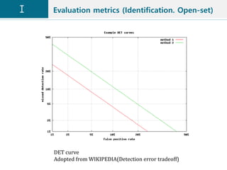
![Evaluation metrics (Identification. Open-set)
• Decision(or Detection) error tradeoff (DET) curve [14]
• Characterize the false negative identification rate(FNIR)
as function of false positive identification rate(FPIR).
• The FPIR measures what fraction of comparisons
between probe templates and non-mate gallery
templates result in a match score exceeding T. At the
same time, the FNIR measures what fraction of probe
searches will fail to match a mated gallery template
above a score of T.
• The algorithms are compared in term of the FNIR at a
low FPIR, e.g. 1% or 10%.
• IJB-A benchmark supports open-set face recognition.](https://image.slidesharecdn.com/facerecognitionv1-190528022819/85/Face-recognition-v1-23-320.jpg)


![Deep FR System
Deep FR System
Adopted from [8].
K. Zhang, Z. Zhang, Z. Li, Y. Qiao. Joint face detection and alignment using multi-task
cascaded convolutional networks. arXiv preprint arXiv:1604.02878, 2016](https://image.slidesharecdn.com/facerecognitionv1-190528022819/85/Face-recognition-v1-28-320.jpg)
![Deep FR System
Adopted from [8].](https://image.slidesharecdn.com/facerecognitionv1-190528022819/85/Face-recognition-v1-29-320.jpg)
![Deep FR System
Adopted from [8].](https://image.slidesharecdn.com/facerecognitionv1-190528022819/85/Face-recognition-v1-30-320.jpg)
![Deep Face (Facebook, CVPR, 2014)
Face Alignment
Adopted from [7].](https://image.slidesharecdn.com/facerecognitionv1-190528022819/85/Face-recognition-v1-31-320.jpg)
![Deep Face (Facebook, CVPR, 2014)
Outline of the DeepFace architecture
Adopted from [7].
Dataset for training: Social Face Classification (SFC) dataset
(4.4M labeled face, 4K identities, 800~1200 faces per person)
Objective: Minimize cross entropy with softmax function.](https://image.slidesharecdn.com/facerecognitionv1-190528022819/85/Face-recognition-v1-32-320.jpg)
![Deep Face (Facebook, CVPR, 2014)
• Verification metric
• Weighted 𝜒2 distance
• DeepFace feature vector contains several similarities
to histogram-based feature.[6]
1. It contains non-negative values
2. It is very sparse
3. Its values are between [0, 1].
• 𝜒2
𝑓1, 𝑓2 = 𝑖
𝑤 𝑖 𝑓1 𝑖 −𝑓2 𝑖 2
𝑓1 𝑖 +𝑓2[𝑖]
• The weight parameters are learned using a linear
SVM.
• Siamese network [18]
• Metric learning
• 𝑑 𝑓1, 𝑓2 = 𝑖 𝛼𝑖|𝑓1 𝑖 − 𝑓2 𝑖 |](https://image.slidesharecdn.com/facerecognitionv1-190528022819/85/Face-recognition-v1-33-320.jpg)
![Deep Face (Facebook, CVPR, 2014)
Adopted from [18].](https://image.slidesharecdn.com/facerecognitionv1-190528022819/85/Face-recognition-v1-34-320.jpg)
![Deep Face (Facebook, CVPR, 2014)
Comparison of the classification errors on the SFC.
Adopted from [7].
• DF-1.5K, 3.3K, 4.4K: Subsets of sizes 1.5K, 3K, 4K persons
• DF-10%, 20%, 50%: the global number of samples in SFC to
10%, 20%, 50%
• DF-sub1, sub2, sub3: chopping off the C3, L4, L5 layers.](https://image.slidesharecdn.com/facerecognitionv1-190528022819/85/Face-recognition-v1-35-320.jpg)
![Deep Face (Facebook, CVPR, 2014)
The performance of various individual DeepFace networks and
the Siamese network.
Adopted from [7].
• DeepFace-single: 3D aligned RGB inputs
• DeepFace-align2D: 2D aligned RGB inputs.
• DeepFace-gradient: gray-level image plus image gradient
magnitude and orientation.
• DeepFace-ensemple: combined distances using a non-linear
SVM with a simple sum of power CPD-kernels.](https://image.slidesharecdn.com/facerecognitionv1-190528022819/85/Face-recognition-v1-36-320.jpg)
![Deep Face (Facebook, CVPR, 2014)
Comparison with the state-of-the-art on the LFW dataset.
Adopted from [7].
• DeepFace-single, unsupervised: directly compare the inner
product of a pair of normalized features.](https://image.slidesharecdn.com/facerecognitionv1-190528022819/85/Face-recognition-v1-37-320.jpg)

![Deep Face (Facebook, CVPR, 2014)
Comparison with the state-of-the-art on the LFW dataset.
Adopted from [7].](https://image.slidesharecdn.com/facerecognitionv1-190528022819/85/Face-recognition-v1-39-320.jpg)

![DeepID2 (CUHK, NIPS, 2014)
The DeepID2 feature learning algorithm.
Adopted from [19].](https://image.slidesharecdn.com/facerecognitionv1-190528022819/85/Face-recognition-v1-41-320.jpg)
![DeepID2 (CUHK, NIPS, 2014)
Patches selected for feature extraction.(positions, scales, color
channels, horizontal flipping)
Adopted from [19].
The ConvNet structure for DeepID2 feature extraction.
Adopted from [19].](https://image.slidesharecdn.com/facerecognitionv1-190528022819/85/Face-recognition-v1-42-320.jpg)

![DeepID2 (CUHK, NIPS, 2014)
(left)Face verification accuracy by varying the weighting
parameter 𝜆.
(right) Face verification accuracy of DeepID2 features learned by
both the face identification and verification signals, where the
number of training identities used for face identification varies.
Adopted from [19].](https://image.slidesharecdn.com/facerecognitionv1-190528022819/85/Face-recognition-v1-44-320.jpg)
![DeepID2 (CUHK, NIPS, 2014)
Spectrum of eigenvalues of the inter- and intra-personal scatter
matrices.
Adopted from [19].](https://image.slidesharecdn.com/facerecognitionv1-190528022819/85/Face-recognition-v1-45-320.jpg)
![DeepID2 (CUHK, NIPS, 2014)
The first two PCA dimensions of DeepID2 features extracted from
six identities in LFW.
Adopted from [19].
Comparison of different verification signals. (classifying the 8192
identities)
Adopted from [19].](https://image.slidesharecdn.com/facerecognitionv1-190528022819/85/Face-recognition-v1-46-320.jpg)
![DeepID2 (CUHK, NIPS, 2014)
Face verification accuracy with DeepID2 features extracted from
an increasing number of face patches.
Adopted from [19].
Accuracy comparison with the previous best results on LFW.
Adopted from [19].](https://image.slidesharecdn.com/facerecognitionv1-190528022819/85/Face-recognition-v1-47-320.jpg)
![DeepID2 (CUHK, NIPS, 2014)
ROC comparison with the previous best results on LFW.
Adopted from [19].](https://image.slidesharecdn.com/facerecognitionv1-190528022819/85/Face-recognition-v1-48-320.jpg)
![DeepID3 (CUHK, arXiv, 2015)
Architecture of DeepID3.
Adopted from [19].](https://image.slidesharecdn.com/facerecognitionv1-190528022819/85/Face-recognition-v1-49-320.jpg)
![DeepID3 (CUHK, arXiv, 2015)
Architecture of DeepID3.
Adopted from [20].](https://image.slidesharecdn.com/facerecognitionv1-190528022819/85/Face-recognition-v1-50-320.jpg)
![DeepID3 (CUHK, arXiv, 2015)
Face verification on LFW.
Adopted from [20].
50 networks.
VGGNet-10](https://image.slidesharecdn.com/facerecognitionv1-190528022819/85/Face-recognition-v1-51-320.jpg)
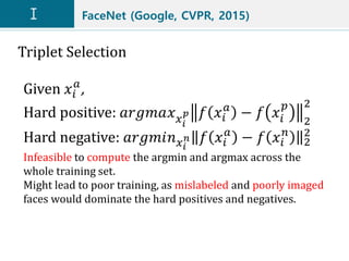
![FaceNet (Google, CVPR, 2015)
Adopted from [21].](https://image.slidesharecdn.com/facerecognitionv1-190528022819/85/Face-recognition-v1-52-320.jpg)


![FaceNet (Google, CVPR, 2015)
Adopted from [21].](https://image.slidesharecdn.com/facerecognitionv1-190528022819/85/Face-recognition-v1-58-320.jpg)
![FaceNet (Google, CVPR, 2015)
Adopted from [21].](https://image.slidesharecdn.com/facerecognitionv1-190528022819/85/Face-recognition-v1-59-320.jpg)
![FaceNet (Google, CVPR, 2015)
Adopted from [21].](https://image.slidesharecdn.com/facerecognitionv1-190528022819/85/Face-recognition-v1-60-320.jpg)
![FaceNet (Google, CVPR, 2015)
Adopted from [21].](https://image.slidesharecdn.com/facerecognitionv1-190528022819/85/Face-recognition-v1-61-320.jpg)
![Center Loss (SIAT, ECCV, 2016)
The distribution of deeply learned features in (a) training set (b) testing set, both under
the supervision of softmax loss.
Adopted from [22].](https://image.slidesharecdn.com/facerecognitionv1-190528022819/85/Face-recognition-v1-62-320.jpg)


![Center Loss (SIAT, ECCV, 2016)
The distribution of deeply learned features under the joint supervision of softmax loss
and center loss.
Adopted from [22].](https://image.slidesharecdn.com/facerecognitionv1-190528022819/85/Face-recognition-v1-65-320.jpg)
![Center Loss (SIAT, ECCV, 2016)
Adopted from [22].](https://image.slidesharecdn.com/facerecognitionv1-190528022819/85/Face-recognition-v1-66-320.jpg)
![Center Loss (SIAT, ECCV, 2016)
Face verification accuracies on LFW dataset, respectively achieve by (a) models with
different 𝜆 and fixed 𝛼 = 0.5. (b) models with different 𝛼 and fixed 𝜆 = 0.003.
Adopted from [22].](https://image.slidesharecdn.com/facerecognitionv1-190528022819/85/Face-recognition-v1-67-320.jpg)
![Center Loss (SIAT, ECCV, 2016)
A: softmax
B:softmax+contrastive
C: proposed. 𝜆 = 0.003, 𝛼 = 0.5
Adopted from [22].](https://image.slidesharecdn.com/facerecognitionv1-190528022819/85/Face-recognition-v1-68-320.jpg)

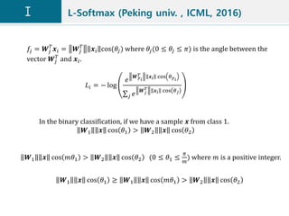
![L-Softmax (Peking univ. , ICML, 2016)
𝐿𝑖 = − log
𝑒
𝑾 𝑦 𝑖
𝑇 𝒙𝑖 𝜓(𝜃 𝑦 𝑖
)
𝑒
𝑾 𝑦 𝑖
𝑇 𝒙𝑖 𝜓(𝜃 𝑦 𝑖
)
+ 𝑗≠𝑦 𝑖
𝑒
𝑾 𝑗
𝑇 𝒙𝑖 cos 𝜃 𝑗
𝜓 𝜃 = −1 𝑘
cos 𝑚𝜃 − 2𝑘, 𝜃 ∈
𝑘𝜋
𝑚
,
𝑘 + 1 𝜋
𝑚
𝑘 ∈ [0, 𝑚 − 1]
Adopted from [23].](https://image.slidesharecdn.com/facerecognitionv1-190528022819/85/Face-recognition-v1-71-320.jpg)
![L-Softmax (Peking univ. , ICML, 2016)
Adopted from [23].
𝑓𝑦 𝑖
=
𝜆 𝑊𝑦 𝑖
𝑥𝑖 cos 𝜃 𝑦 𝑖
+ 𝑊𝑦 𝑖
𝑥𝑖 𝜓 𝜃 𝑦 𝑖
1 + 𝜆](https://image.slidesharecdn.com/facerecognitionv1-190528022819/85/Face-recognition-v1-72-320.jpg)
![L-Softmax (Peking univ. , ICML, 2016)
Adopted from [23].
cos(𝑛𝑥) =
𝑘=0
𝑛
2
−1 𝑘 𝑛
2𝑘
sin2 𝑥 𝑘 cos 𝑛−2𝑘(𝑥)
=
𝑘=0
𝑛
2
−1 𝑘 𝑛
2𝑘
1 − cos2
𝑥 𝑘
cos 𝑛−2𝑘
(𝑥)
For forward and backward propagation, we need to replace cos(𝜃𝑗) with
𝑾 𝑗
𝑇
𝒙 𝑖
𝑾 𝑗
𝑇 𝒙𝑖
cos(𝑚𝜃 𝑦 𝑖
)
=
𝑚
0
cos 𝑚(𝜃 𝑦 𝑖
) −
𝑚
2
cos 𝑚−2 𝜃 𝑦 𝑖
1 − cos2 𝜃 𝑦 𝑖
+
𝑚
4
cos 𝑚−4 𝜃 𝑦 𝑖
1 − cos2 𝜃 𝑦 𝑖
2
+ ⋯ −1 𝑛 𝑚
2𝑛
cos 𝑚−2𝑛
𝜃 𝑦 𝑖
1 − cos2
𝜃 𝑦 𝑖
𝑛
+ ⋯
Where 𝑛 is an integer and 2𝑛 ≤ 𝑚.](https://image.slidesharecdn.com/facerecognitionv1-190528022819/85/Face-recognition-v1-73-320.jpg)
![L-Softmax (Peking univ. , ICML, 2016)
Adopted from [23].](https://image.slidesharecdn.com/facerecognitionv1-190528022819/85/Face-recognition-v1-74-320.jpg)
![L-Softmax (Peking univ. , ICML, 2016)
Adopted from [23].](https://image.slidesharecdn.com/facerecognitionv1-190528022819/85/Face-recognition-v1-75-320.jpg)
![L-Softmax (Peking univ. , ICML, 2016)
Adopted from [23].](https://image.slidesharecdn.com/facerecognitionv1-190528022819/85/Face-recognition-v1-76-320.jpg)
![SphereFace (Georgia Tech. , CVPR, 2017)
Adopted from [24].
𝐿𝑖 = − log
𝑒 𝒙𝑖 𝜓(𝜃 𝑦 𝑖
)
𝑒 𝒙𝑖 𝜓(𝜃 𝑦 𝑖
)
+ 𝑗≠𝑦 𝑖
𝑒 𝒙 𝑖 cos 𝜃 𝑗
𝜓 𝜃 = −1 𝑘 cos 𝑚𝜃 − 2𝑘, 𝜃 ∈
𝑘𝜋
𝑚
,
𝑘 + 1 𝜋
𝑚
𝑘 ∈ [0, 𝑚 − 1]
In the binary classification.
𝑾1 = 𝑾2 = 1](https://image.slidesharecdn.com/facerecognitionv1-190528022819/85/Face-recognition-v1-77-320.jpg)
![SphereFace (Georgia Tech. , CVPR, 2017)
Adopted from [24].](https://image.slidesharecdn.com/facerecognitionv1-190528022819/85/Face-recognition-v1-78-320.jpg)
![SphereFace (Georgia Tech. , CVPR, 2017)
Adopted from [24].](https://image.slidesharecdn.com/facerecognitionv1-190528022819/85/Face-recognition-v1-79-320.jpg)
![SphereFace (Georgia Tech. , CVPR, 2017)
Adopted from [24].](https://image.slidesharecdn.com/facerecognitionv1-190528022819/85/Face-recognition-v1-80-320.jpg)
![SphereFace (Georgia Tech. , CVPR, 2017)
Experiments on LFW and YTF.
Adopted from [24].](https://image.slidesharecdn.com/facerecognitionv1-190528022819/85/Face-recognition-v1-81-320.jpg)
![SphereFace (Georgia Tech. , CVPR, 2017)
MegaFace.
Adopted from [24].](https://image.slidesharecdn.com/facerecognitionv1-190528022819/85/Face-recognition-v1-82-320.jpg)
![SphereFace (Georgia Tech. , CVPR, 2017)
Experiments on MegaFace
Adopted from [24].](https://image.slidesharecdn.com/facerecognitionv1-190528022819/85/Face-recognition-v1-83-320.jpg)
![SphereFace (Georgia Tech. , CVPR, 2017)
1:1M rank-1 identification results on MegaFace benchmark: (a)
introducing label flips to training data, (b) introducing outliers to
training data.
Adopted from [26].](https://image.slidesharecdn.com/facerecognitionv1-190528022819/85/Face-recognition-v1-84-320.jpg)
![CosFace (Tencent AI Lab, arXiv, 2018)
Adopted from [25].](https://image.slidesharecdn.com/facerecognitionv1-190528022819/85/Face-recognition-v1-85-320.jpg)
![CosFace (Tencent AI Lab, arXiv, 2018)
Adopted from [25].](https://image.slidesharecdn.com/facerecognitionv1-190528022819/85/Face-recognition-v1-86-320.jpg)
![CosFace (Tencent AI Lab, arXiv, 2018)
Adopted from [25].](https://image.slidesharecdn.com/facerecognitionv1-190528022819/85/Face-recognition-v1-87-320.jpg)
![CosFace (Tencent AI Lab, arXiv, 2018)
Adopted from [25].](https://image.slidesharecdn.com/facerecognitionv1-190528022819/85/Face-recognition-v1-88-320.jpg)
![CosFace (Tencent AI Lab, arXiv, 2018)
Adopted from [25].](https://image.slidesharecdn.com/facerecognitionv1-190528022819/85/Face-recognition-v1-89-320.jpg)
![CosFace (Tencent AI Lab, arXiv, 2018)
Adopted from [25].](https://image.slidesharecdn.com/facerecognitionv1-190528022819/85/Face-recognition-v1-90-320.jpg)
![L2-normalization, scaling
Adopted from [27].](https://image.slidesharecdn.com/facerecognitionv1-190528022819/85/Face-recognition-v1-91-320.jpg)
![ArcFace (Imperial College, arXiv, 2018)
Adopted from [28].](https://image.slidesharecdn.com/facerecognitionv1-190528022819/85/Face-recognition-v1-92-320.jpg)
![ArcFace (Imperial College, arXiv, 2018)
Adopted from [28].](https://image.slidesharecdn.com/facerecognitionv1-190528022819/85/Face-recognition-v1-93-320.jpg)
![ArcFace (Imperial College, arXiv, 2018)
Adopted from [28].](https://image.slidesharecdn.com/facerecognitionv1-190528022819/85/Face-recognition-v1-94-320.jpg)
![ArcFace (Imperial College, arXiv, 2018)
Adopted from [28].](https://image.slidesharecdn.com/facerecognitionv1-190528022819/85/Face-recognition-v1-95-320.jpg)
![ArcFace (Imperial College, arXiv, 2018)
Adopted from [28].](https://image.slidesharecdn.com/facerecognitionv1-190528022819/85/Face-recognition-v1-96-320.jpg)
![ArcFace (Imperial College, arXiv, 2018)
Adopted from [28].](https://image.slidesharecdn.com/facerecognitionv1-190528022819/85/Face-recognition-v1-97-320.jpg)
![ArcFace (Imperial College, arXiv, 2018)
Adopted from [28].](https://image.slidesharecdn.com/facerecognitionv1-190528022819/85/Face-recognition-v1-98-320.jpg)
![ArcFace (Imperial College, arXiv, 2018)
Adopted from [28].](https://image.slidesharecdn.com/facerecognitionv1-190528022819/85/Face-recognition-v1-99-320.jpg)
![ArcFace (Imperial College, arXiv, 2018)
Adopted from [28].](https://image.slidesharecdn.com/facerecognitionv1-190528022819/85/Face-recognition-v1-100-320.jpg)
![ArcFace (Imperial College, arXiv, 2018)
Adopted from [28].](https://image.slidesharecdn.com/facerecognitionv1-190528022819/85/Face-recognition-v1-101-320.jpg)
![ArcFace (Imperial College, arXiv, 2018)
Adopted from [28].](https://image.slidesharecdn.com/facerecognitionv1-190528022819/85/Face-recognition-v1-102-320.jpg)
![ArcFace (Imperial College, arXiv, 2018)
Adopted from [28].](https://image.slidesharecdn.com/facerecognitionv1-190528022819/85/Face-recognition-v1-103-320.jpg)
![ArcFace (Imperial College, arXiv, 2018)
Adopted from [28].](https://image.slidesharecdn.com/facerecognitionv1-190528022819/85/Face-recognition-v1-104-320.jpg)
![ArcFace (Imperial College, arXiv, 2018)
Adopted from [28].](https://image.slidesharecdn.com/facerecognitionv1-190528022819/85/Face-recognition-v1-105-320.jpg)
![ArcFace (Imperial College, arXiv, 2018)
Adopted from [28].](https://image.slidesharecdn.com/facerecognitionv1-190528022819/85/Face-recognition-v1-106-320.jpg)
![References
[1] M. Turk, A. Pentland, “Face recognition using eigenfaces,” in Proc. CVPR, pp.
586–591. (1991)
[2] P. Belhumeur, J. P. Hespanha, and D. Kriegman. “Eigenfaces vs. fisherfaces:
Recognition using class specific linear projection,” in PAMI, 19(7):711-720, July
1997.
[3] H. G. Feichtinger, T. Strohmer, “Gabor Analysis and Algorithms,” in Birkhauser,
1998.
[4] DC. He, L. Wang, “Texture Unit, Texture Spectrum, And Texture Analysis,” in
IEEE Trans. Geoscience and Remote Sensing, Vol. 8, No. 8, pp. 905-910, 1990.
[5] L. Wang, DC. He, “Texture Classification Using Texture Spectrum,” in Pattern
Recognition, Vol. 23, No. 8, pp. 905-910, 1990.
[6] T. Ahonen, A. Hadid, and M. Pietikainen, “Face description with local binary
patterns: Application to face recognition,” in PAMI, 2006
[7] Y. Taigman, M. Yang, M. Ranzato, L. Wolf, “DeepFace: Closing the gap to human-
level performance in face verification,” in Proc. CVPR, 2014
[8] M. Wang, W. Deng, “Deep Face Recognition: A Survey,” ArXiv preprint
arXiv:1804.06655v8
[9] W. Liu, Y. Wen, Z. Yu, M. Li, B. Raj, L. Song, SphereFace: Deep Hypersphere
Embedding for Face Recognition. In Conf. on CVPR, 2017](https://image.slidesharecdn.com/facerecognitionv1-190528022819/85/Face-recognition-v1-107-320.jpg)
![References
[10] G. B. Huang, M. Ramesh, T. Berg, E. Learned-Miller. Labeled Faces in the Wild:
A Database for Studying Face Recognition in Unconstrained Environments.
University of Massachusetts, Amherst, Technical Report 07-49, October, 2007.
[11] G. B. Huang, E. Learned-Miller. Labeled Faces in the Wild: Updates and New
Reporting Procedures.
[12] J. Deng, J. Guo, S. Zafeiriou. Arcface: Additive angular margin loss for deep
face recognition. arXiv preprint arXiv:1712.04695, 2017
[13] F. Zhao & Y. Jian, Y. Shuicheng, J. Feng. Dynamic Conditional Networks for
Few-Shot Learning. ECCV, 2018
[14] B. K. Klare, B. Klein, E. Taborsky, A. Blanton, J. Cheney, K. Allen, P. Grother, A.
Mah, K. Jain. Pushing the Frontiers of Unconstrained Face Detection and
Recognition: IARPA Janus Benchmark A. CVPR, 2015
[15] A. Talwalkar, S. Kumar, H. Rowley. Large-scale manifold learning. In CVPR,
2014
[16] K. –C. Lee, J. Ho, M. –H. Yang, D. Kriegman. Video-based face recognition using
probabilistic appearance minifolds. In CVPR, 2003.
[17] X. He, S. Yan, Y. Hu, P. Niyogi, H.-J. Zhang. “Face recognition using
laplacianfaces,” PAMI, 27(3):328-240.
[18] S. Chopra, R. Hadsell, Y. LeCun. Learning a similarity metric discriminatively,
with application to face verification. In CVPR, 2005.](https://image.slidesharecdn.com/facerecognitionv1-190528022819/85/Face-recognition-v1-108-320.jpg)
![References
[19] Y. Sun, Y. Chen, X. Wang, X. Tang. Deep learning face representation by joint
identification-verification. In NIPS, pages 1988-1996, 2014.
[20] Y. Sun, D. Liang, X. Wang, X. Tang. Deepid3: Face recognition with very deep
neural networks. arXiv preprint arXiv:1502.00873
[21] F. Schroff, D. Kalenichenko, J. Philbin. Facenet: A unified embedding for face
recognition and clustering. In CVPR, pp. 815-823, 2015.
[22] Y. Wen, K. Zhang, Z. Li, Y. Qiao. A discriminative feature learning approach for
deep face recognition. In ECCV, pp 299-515, 2016.
[23] W. Liu, Y. Wen, Z. Yu, M. Yang. Large-margin softmax loss for convolutional
neural networks. In ICML, pp. 507-516, 2016.
[24] W. Liu, Y. Wen, Z. Yu, M. Li, B. Raj, L. Song. Sphererface: Deep hypersphere
embedding for face recognition. In CVPR, volume 1, 2017.
[25] F. Wang, W. Liu, H. Liu, J. Cheng. Additive margin softmax for face verification.
arXiv preprint arXiv:1801.05599, 2018
[26] F. Wang, L. Chen, C. Li, S. Huang, Y. Chen, C. Qian, C. Change Loy. The devil of
face recognition is in the noise. In ECCV, September 2018.
[27] R. Ranjan, C. D. Castillo, R. Chellappa. L2-constrained softmax loss for
discriminative face verification. arXiv preprint arXiv:1703.09507, 2017.
[28] J. Deng, J. Guo, S. Zafeiriou. Arcface: Additive angular margin loss for deep
face recognition .arXiv:1801.07698, 2018.](https://image.slidesharecdn.com/facerecognitionv1-190528022819/85/Face-recognition-v1-109-320.jpg)


![SSII2021 [SS1] Transformer x Computer Visionの 実活用可能性と展望 〜 TransformerのCompute...](https://cdn.slidesharecdn.com/ss_thumbnails/ss1-01-210607043349-thumbnail.jpg?width=640&height=640&fit=bounds)