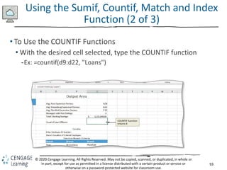
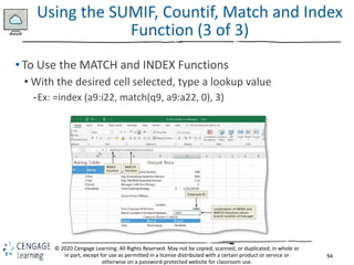
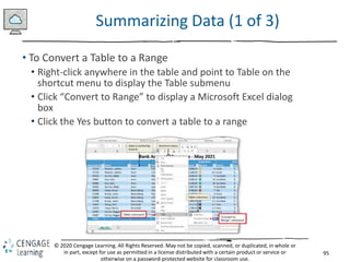
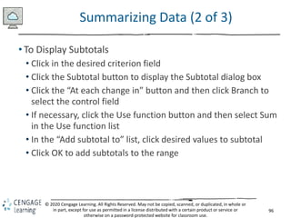
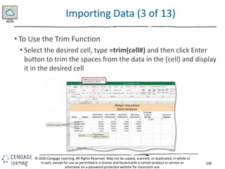
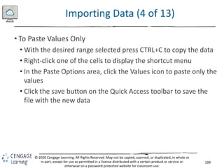
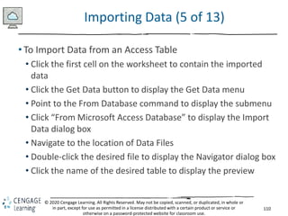
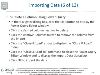
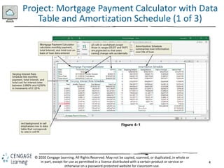
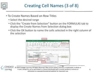
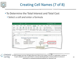
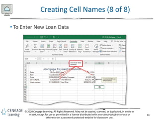
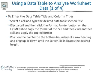
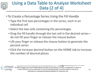
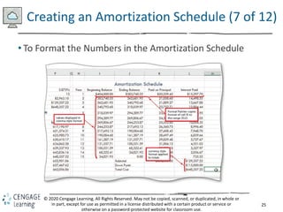
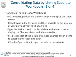
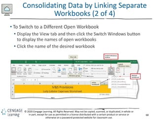
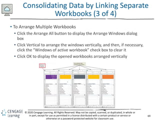
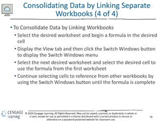
The document covers Microsoft Excel 2019's financial functions and data manipulation, including creating amortization schedules and data tables. It outlines objectives such as calculating loan payments using functions like PMT and managing worksheet formatting. It also includes detailed steps for projects like a mortgage payment calculator and formatting data for analysis.


![48
© 2020 Cengage Learning. All Rights Reserved. May not be copied, scanned, or duplicated, in whole or
in part, except for use as permitted in a license distributed with a certain product or service or
otherwise on a password-protected website for classroom use.
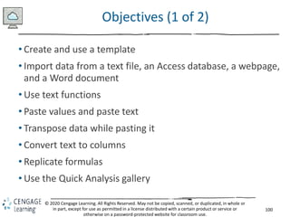
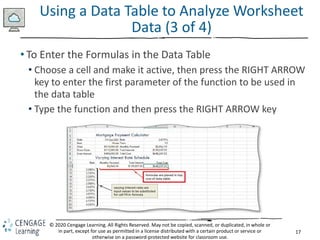
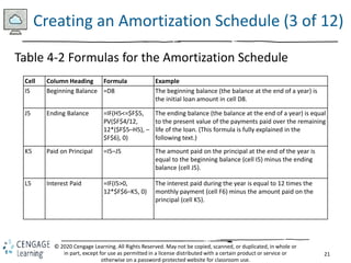
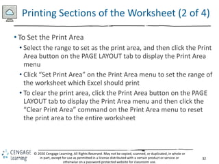
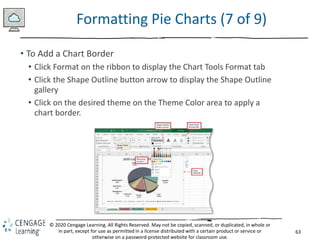
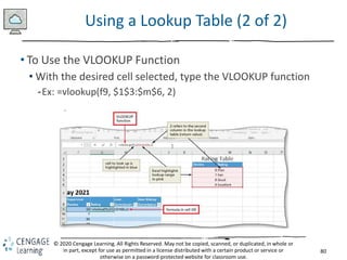
Format Codes (1 of 2)
Table 5-5 Format Symbols in Format Codes
Format Symbol Example of
Symbol in Code
Description
# (number
sign)
###.## Serves as a digit placeholder. If the value in a cell has more digits to the right of the decimal point
than number signs in the format, Excel rounds the number. All digits to the left of the decimal point
are displayed.
0 (zero) 0.00 Works like a number sign (#), except that if the number is less than 1, Excel displays a 0 in the ones
place.
. (period) #0.00 Ensures Excel will display a decimal point in the number. The placement of zeros determines how
many digits appear to the left and right of the decimal point.
% (percent) 0.00% Displays numbers as percentages of 100. Excel multiplies the value of the cell by 100 and displays a
percent sign after the number.
, (comma) #,##0.00 Displays a comma as a thousands separator.
( ) #0.00;(#0.00) Displays parentheses around negative numbers.
$, +, or – $#,##0.00;
($#,##0.00)
Displays a floating sign ($, +, or –).
* (asterisk) $*##0.00 Displays a fixed sign ($, +, or –) to the left, followed by spaces until the first significant digit.
[color] #.##;[Red]#.## Displays the characters in the cell in the designated color. In the example, positive numbers appear
in the default color, and negative numbers appear in red.
” ” (quotation
marks)
$0.00 “Surplus”; $-
0.00 “Shortage”
Displays text along with numbers entered in a cell.
_ (underscore) #,##0.00_) Adds a space. When followed by a parentheses, positive numbers will align correctly with
parenthetical negative numbers.](https://image.slidesharecdn.com/excelmodules4-7-240504223041-1d0b1254/85/Excel-Modules-4-7-Microsoft-Excel-Shelly-Cashman-pptx-48-320.jpg)


![81
© 2020 Cengage Learning. All Rights Reserved. May not be copied, scanned, or duplicated, in whole or
in part, except for use as permitted in a license distributed with a certain product or service or
otherwise on a password-protected website for classroom use.
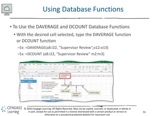
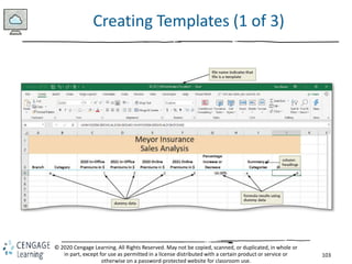
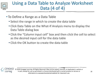
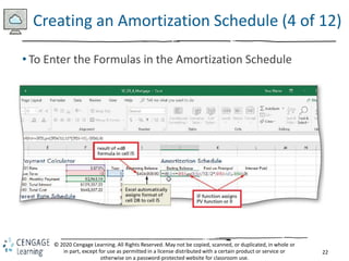
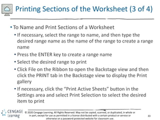
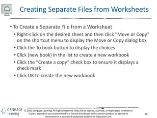
Adding Calculated Fields to the Table
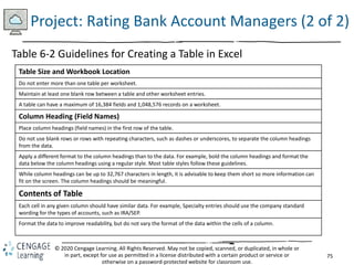
• To Create Calculated Fields
• Click the desired cell
• Click the “Accounting Number Format” button so that data in
the selected column is displayed as a dollar amount with two
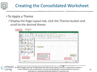
decimal places
• Double-click Specialty to select the field to use for the IF
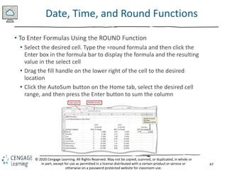
function
• Type =IF([Specialty]=“Loans”,[Account Values] * .0025, 0) to
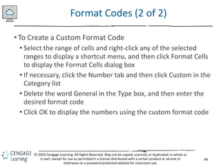
complete the structured reference and then click the Enter
button to create the calculated column](https://image.slidesharecdn.com/excelmodules4-7-240504223041-1d0b1254/85/Excel-Modules-4-7-Microsoft-Excel-Shelly-Cashman-pptx-81-320.jpg)