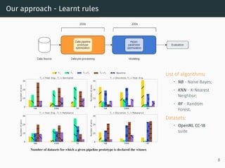
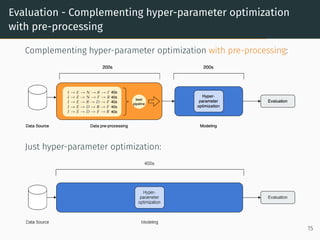
The document discusses effective data pre-processing techniques for automated machine learning (AutoML), emphasizing the importance of optimized data pipelines and algorithm configurations. It presents a framework for selecting data transformations, evaluates the effectiveness of these prototypes, and highlights that pre-processing optimization can significantly enhance predictive accuracy while being cost-effective. Future work aims to explore datasets that are less responsive to pre-processing and to integrate a meta-learning module into the approach.

1. Effective data pre-processing for AutoML
Joseph Giovanelli Besim Bilalli Alberto Abelló
j.giovanelli@unibo.it bbilalli@essi.upc.edu aabello@essi.upc.edu

2. The data analytics process
Based on the problem to tackle:
• Data Pipeline Selection and Optimization (DPSO) 1
consists of
finding the best data pipeline;
• Combined Algorithm Selection and Hyperparameter
Optimization (CASH) 2
consists of finding the best algorithm and
its configuration.
1Alexandre Quemy. 2020. Two-stage optimization for machine learning workflow. Information
Systems 92 (2020).
2Chris Thornton, Frank Hutter, Holger H. Hoos, et al. 2013. Auto-WEKA: Combined Selection and
Hyperparameter Optimization of Classification Algorithms. In KDD.
1

3. AutoML and data analytics process
Automated Machine Learning (AutoML) aims to automate the whole
data analytics process.
Highlight:
• usage of state-of-the-art
optimization techniques e.g.,
Sequential Model-Based
Optimization (SMBO) 3
Drawback:
• neglect of data
pre-processing
1Frank Hutter, Holger H Hoos, and Kevin Leyton-Brown. 2011. Sequential model-based
optimization for general algorithm configuration. In International conference on learning and
intelligent optimization.Springer, 507–523.
2

4. Data pre-processing complexity
List of transformations:
• E - Encoding;
• N - Normalization;
• D - Discretization;
• I - Imputation;
• R - Rebalancing;
• F - Feature Engineering.
framework=
scikit-learn 4
Framework-related rules:
1 - a precedence edge exists between
the row and the column,
0 - a precedence edge does not exist
between the row and the column,
x - the combination is meaningless.
2https://scikit-learn.org/stable/
3

5. Data pre-processing complexity
Framework-related rules:
1 - a precedence edge exists between
the row and the column,
0 - a precedence edge does not exist
between the row and the column,
x - the combination is meaningless.
Exhaustive set of data pipeline prototypes:
4

6. Data pre-processing complexity - Universal pipeline prototype
List of algorithms:
• NB - Naive Bayes;
• KNN - K-Nearest
Neighbor;
• RF - Random
Forest.
Datasets:
• OpenML CC-18
suite 5
3https://www.openml.org/s/99
5

7. Our approach

8. Our approach
1. Build effective pipeline prototypes:
2. Optimize them
3. Select the best one
6

9. Our approach - Building effective pipeline prototypes
Framework-related rules: Heuristic rules: Learnt rules:
E - Encoding N - Normalization D - Discretization I - Imputation R - Rebalancing F - Feature Eng.
1 - a precedence edge exists between the row and the column,
0 - a precedence edge does not exist between the row and the column,
x - the combination is meaningless.
7

10. Our approach - Learnt rules
List of algorithms:
• NB - Naive Bayes;
• KNN - K-Nearest
Neighbor;
• RF - Random
Forest.
Datasets:
• OpenML CC-18
suite
8

11. Our approach - Building effective pipeline prototypes
Framework-related rules: Heuristic rules: Learnt rules:
E - Encoding N - Normalization D - Discretization I - Imputation R - Rebalancing F - Feature Eng.
1 - a precedence edge exists between the row and the column, 0 - a precedence edge does not exist between the row and the column,
x - the combination is meaningless.
Union of rules:
9

12. Our approach - Building effective pipeline prototypes
Union of rules:
1 - a precedence edge exists between
the row and the column,
0 - a precedence edge does not exist
between the row and the column,
x - the combination is meaningless.
Effective set of data pipeline prototypes:
10

13. Our approach - Optimization
11

14. Evaluation

15. Evaluation - Effective versus exhaustive prototypes optimization
Effective prototypes optimization (our approach):
Exhaustive prototypes optimization :
for each of the possible
data pipeline prototypes:
12

16. Evaluation - Effective versus exhaustive prototypes optimization
normalized distance =
Acc(deffective, a∗
) − Acc(d, a)
Acc(dexhaustive, a∗) − Acc(d, a)
• Acc(d, a): baseline accuracy (i.e., predictive accuracy of the algorithm a
with default hyper-parameters over the original dataset d);
• Acc(deffective, a∗
): accuracy of the optimized algorithm a∗
over the
dataset deffective transformed using the optimized instantiation of the
effective set of prototypes obtained with our approach;
• Acc(dexhaustive, a∗
): accuracy of the optimized algorithm a∗
over the
dataset dexhaustive transformed using the optimized pipeline
instantiation of the exhaustive set of prototypes.
13

17. Evaluation - Effective versus exhaustive prototypes optimization
normalized distance =
Acc(deffective, a∗
) − Acc(d, a)
Acc(dexhaustive, a∗) − Acc(d, a)
Normalized distances
between the scores
obtained by
optimizing our
effective prototypes
and the ones
obtained optimizing
the exhaustive set.
14

18. Evaluation - Complementing hyper-parameter optimization
with pre-processing
Complementing hyper-parameter optimization with pre-processing:
Just hyper-parameter optimization:
15

19. Evaluation - Complementing hyper-parameter optimization
with pre-processing
pp impact =
Acc(deffective, a∗
) − Acc(d, a)
max(Acc(deffective, a∗), Acc(d, a∗)) − Acc(d, a)
hp impact =
Acc(d, a∗
) − Acc(d, a)
max(Acc(deffective, a∗), Acc(d, a∗)) − Acc(d, a)
• Acc(d, a): baseline accuracy (i.e., predictive accuracy of the algorithm a
with default hyper-parameters over the original dataset d);
• Acc(deffective, a∗
): accuracy of the optimized algorithm a∗
over the
dataset deffective transformed using the optimized instantiation of the
effective set of prototypes obtained with our approach;
• Acc(d, a∗
): accuracy of the optimized algorithm a∗
(i.e, using the entire
budget) over the original dataset d.
16

20. Evaluation - Complementing hyper-parameter optimization
with pre-processing
normalized pp impact =
pp impact
pp impact + hp impact
normalized hp impact =
hp impact
pp impact + hp impact
17

21. Conclusions and future works
Contributions:
• no universal pre-processing pipeline prototype;
• pre-processing optimization may boost the final result;
• our approach provides results that get 90% of the optimal
predictive accuracy in the median, but with a cost that is 24
times smaller;
Future works:
• study the datasets that do not react well to data-pre-processing;
• extend our approach with a meta-learning module.
18

22. Thanks for the attention
18