Economic roots (1)

Journal of Economic Literature 2013, 51(2), 325–369
http://dx.doi.org/10.1257/jel.51.2.325
325
“The further backward you look,
the further forward you can see”
(attributed to Winston Churchill).1
1. Introduction
W hy is income per capita higher in
some societies and much lower in
others? Answers to this perennial question
have evolved over time. Decades ago, the
emphasis was on the accumulation of fac-
tors of production and exogenous techno-
logical progress. Later, the focus switched
to policies and incentives endogenously
affecting factor accumulation and innova-
tion. More recently, the attention has moved
to the institutional framework underly-
ing these policies and incentives. Pushing
How Deep Are the Roots
of Economic Development?†
Enrico Spolaore and Romain Wacziarg*
The empirical literature on economic growth and development has moved from the
study of proximate determinants to the analysis of ever deeper, more fundamental
factors, rooted in long-term history. A growing body of new empirical work focuses on
the measurement and estimation of the effects of historical variables on contemporary
income by explicitly taking into account the ancestral composition of current
populations. The evidence suggests that economic development is affected by traits
that have been transmitted across generations over the very long run. This article
surveys this new literature and provides a framework to discuss different channels
through which intergenerationally transmitted characteristics may impact economic
development, biologically (via genetic or epigenetic transmission) and culturally (via
behavioral or symbolic transmission). An important issue is whether historically
transmitted traits have affected development through their direct impact on
productivity, or have operated indirectly as barriers to the diffusion of productivity-
enhancing innovations across populations. (JEL J11, O33, O47, Z13)
* Spolaore: Tufts University, National Bureau of Eco-
nomic Research, and CESIfo. Wacziarg: University of
California at Los Angeles, National Bureau of Economic
Research, and CEPR. We thank Leonardo Bursztyn, Janet
Currie, Oded Galor, David Weil, and several anonymous
referees for useful input.
†
Go to http://dx.doi.org/10.1257/jel.51.2.325 to visit the
article page and view author disclosure statement(s).
1 This is the usual form of the quote attributed to
Winston Churchill—for instance, by Queen Elizabeth II
in her 1999 Christmas Message. According to Langworth
(2008, 577), Churchill’s words were “the longer you can
look back, the farther you can look forward.”

Journal of Economic Literature, Vol. LI (June 2013)326
back the debate one more degree, a key
question remains as to why the proximate
determinants of the wealth of nations vary
across countries. A burgeoning literature
seeks to better understand the deep causes
of development, rooted in geography and
history.
As the empirical literature has moved
from studying the proximate determi-
nants of growth and development to ana-
lyzing ever deeper, more fundamental
factors, important questions have arisen:
How much time persistence is there in
development outcomes? How far back in
time should we go in order to understand
contemporary economic development?
Through what specific mechanisms do
long-term geographic and historical fac-
tors affect outcomes today? If economic
development has deep historical roots,
what is the scope for policy to affect the
wealth of nations? This article discusses
the current state of knowledge on these
issues, focusing on recent empirical work
shedding light on the complex interactions
among geography, history, and compara-
tive development. Throughout, we illus-
trate the major milestones of the recent
literature in a unified empirical frame-
work for understanding variation in eco-
nomic development.
Our starting point is the long-standing
debate on geography and development.
There is no doubt that geographic factors,
such as latitude and climate, are highly cor-
related with development, but the inter-
pretation of this correlation remains hotly
debated. While some of the effects of geog-
raphy may operate directly on current pro-
ductivity, there is mounting evidence that
much of the correlation operates through
indirect mechanisms, i.e., through the his-
torical effects of initial geographic condi-
tions on the spatial distribution of human
characteristics, such as institutions, human
capital, social capital, and cultural traits,
affecting income and productivity over
the long run.2
We review the literature
on the legacy of geographic conditions in
section 2.
A major theme emerging from the recent
literature is that key human characteristics
affecting development are transmitted from
one generation to the next within popula-
tions over the long run, explaining why deep
historical factors still affect outcomes today.
A growing body of new empirical work has
focused on the measurement and estimation
of long-term effects of historical variables
on contemporary income by explicitly tak-
ing into account the ancestral composition of
current populations (Spolaore and Wacziarg
2009; Putterman and Weil 2010; Comin,
Easterly, and Gong 2010; Ashraf and Galor
2013). We survey contributions to this new
literature in section 3.
In section 4, we provide a general taxon-
omy to discuss different channels through
which inherited human characteristics may
impact economic development. Our discus-
sion builds on an extensive evolutionary lit-
erature on the complex interactions among
genetic, epigenetic, and cultural transmis-
sion mechanisms, and on the coevolution of
biological and cultural traits (Cavalli-Sforza
and Feldman 1981; Boyd and Richerson
1985; Richerson and Boyd 2005; Jablonka
and Lamb 2005), as well as on a growing
literature on cultural transmission and eco-
nomic outcomes (e.g., Bisin and Verdier
2000, 2001; Tabellini 2008, 2009; Alesina,
Giuliano, and Nunn 2013). An important
issue is whether historically transmitted
characteristics affect economic development
through their direct impact on productivity,
or operate indirectly as barriers to the diffu-
sion of technological and institutional inno-
vations across populations.
2 For recent discussions of these issues from differ-
ent perspectives, see Galor (2005, 2011) and Acemoglu,
Johnson, and Robinson (2005).

327Spolaore and Wacziarg: How Deep Are the Roots of Economic Development?
2. Geography and Development
2.1 Long-Term Effects of Geography
The hypothesis that geographic factors
affect productivity and economic develop-
ment has a long pedigree, going back to
Machiavelli (1531), Montesquieu (1748), and
Marshall (1890). A vast empirical literature
has documented high correlations between
current levels of income per capita and a
series of geographic and biological variables,
such as climate and temperature (Myrdal
1968; Kamarck 1976; Masters and McMillan
2001; Sachs 2001), the disease environment
(Bloom and Sachs 1998; Sachs, Mellinger,
and Gallup 2001; Sachs and Malaney 2002),
natural resources (Sachs and Warner 2001),
and transportation conditions (Rappaport
and Sachs 2003).
In order to illustrate the main empiri-
cal findings of the contributions discussed
herein, we punctuate this paper with our
own empirical results based on a unified data
set, regression methodology and sample.
This analysis is not meant to be an exhaustive
recapitulation of existing results, but simply
to illustrate some important milestones in
the recent literature. We use, alternately, log
per capita income in 2005 (from the Penn
World Tables version 6.3) as a measure of
contemporary economic performance, and
population density in 1500 (from McEvedy
and Jones 1978) as a measure of economic
performance in 1500, and regress these on a
variety of proposed determinants of develop-
ment, starting here with geographic factors.3
3 As is well known, in the preindustrial, Malthusian
era population density is the appropriate measure of a
society’s economic performance since any technologi-
cal improvement leads to increases in population rather
than to increases in per capita income. For a theoretical
and empirical analysis of the relationship between popu-
lation size, population density, and long-term growth in
Malthusian times, see Kremer (1993). For in-depth discus-
sions of this topic, see Galor (2005) and the recent contri-
bution by Ashraf and Galor (2011a).
Table 1, column 1 shows that a small set of
geographic variables (absolute latitude, the
percentage of a country’s land area located
in tropical climates, a landlocked coun-
try dummy, an island country dummy) can
jointly account for 44 percent of contempo-
rary variation in log per capita income, with
quantitatively the largest effect coming from
absolute latitude (excluding latitude causes
the R2
to fall to 0.29). This result captures
the flavor of the above-cited literature docu-
menting a strong correlation between geog-
raphy and income per capita.
While the correlation between geography
and development is well established, the
debate has centered around causal mecha-
nisms. A number of prominent economists,
including Myrdal (1968), Kamarck (1976),
and Sachs and coauthors, argue that geo-
graphic factors have a direct, contemporane-
ous effect on productivity and development.
In particular, Sachs (2001) claims that eco-
nomic underdevelopment in tropical coun-
tries can be partly explained by the current
negative effects of their location, which
include two main ecological handicaps: low
agricultural productivity and a high burden of
diseases. Tropical soils are depleted by heavy
rainfall, and crops are attacked by pests and
parasites that thrive in hot climates without
winter frosts (Masters and McMillan 2001).
Warm climates also favor the transmission of
tropical diseases borne by insects and bacte-
ria, with major effects on health and human
capital. In sum, according to this line of
research, geography has direct current effects
on productivity and income per capita.
Other scholars, in contrast, claim that
geography affects development indirectly
through historical channels, such as the
effects of prehistoric geographic and biologi-
cal conditions on the onset and spread of agri-
culture and domestication (Diamond 1997;
Olsson and Hibbs 2005), and the effects
of crops and germs on the settlement of
European colonizers after 1500 (Engerman

and Sokoloff 1997 and 2002; Acemoglu,
Johnson, and Robinson 2001, 2002; Easterly
and Levine 2003).
Diamond (1997) famously argues that the
roots of comparative development lie in a
series of environmental advantages enjoyed
by the inhabitants of Eurasia at the transition
from a hunter–gatherer economy to agricul-
tural and pastoral production, starting roughly
in 10,000 BC (the Neolithic Revolution).
These advantages included the larger size
of Eurasia, its initial biological conditions
(the diversity of animals and plants avail-
able for domestication in prehistoric times),
and its East–West orientation, which facili-
tated the spread of agricultural innovations.
Building on these geographic advantages,
Eurasia experienced a population explosion
Table 1
Geography and Contemporary Development
(Dependent variable: log per capita income, 2005; estimator: OLS)
Sample:
Whole
World
Olsson–Hibbs
samplea
Olsson–Hibbs
samplea
Olsson–Hibbs
samplea
Olsson–Hibbs
samplea
Old World
only
(1) (2) (3) (4) (5) (6)
Absolute latitude 0.044 0.052
(6.645)*** (7.524)***
Percent land area in –0.049 0.209 –0.410 –0.650 –0.421 –0.448
the tropics (0.154) (0.660) (1.595) (2.252)** (1.641) (1.646)
Landlocked dummy –0.742 –0.518 –0.499 –0.572 –0.505 –0.226
(4.375)*** (2.687)*** (2.487)** (2.622)** (2.523)** (1.160)
Island dummy 0.643 0.306 0.920 0.560 0.952 1.306
(2.496)** (1.033) (3.479)*** (1.996)** (3.425)*** (4.504)***
Geographic conditions 0.706 0.768 0.780
(Olsson–Hibbs)b
(6.931)*** (4.739)*** (5.167)***
Biological conditions 0.585 –0.074 0.086
(Olsson–Hibbs)c
(4.759)*** (0.483) (0.581)
Constant 7.703 7.354 8.745 8.958 8.741 8.438
(25.377)*** (25.360)*** (61.561)*** (58.200)*** (61.352)*** (60.049)***
Observations 155 102 102 102 102 83
Adjusted R2
0.440 0.546 0.521 0.449 0.516 0.641
Notes:
a
The Olsson and Hibbs sample excludes the neo-European countries (Australia, Canada, New Zealand, and the
United States) and countries whose current income is based primarily on extractive wealth (Olsson and Hibbs 2005).
b
First principal component of number of annual or perennial wild grasses and number of domesticable big mam-
mals (all variables from Olsson and Hibbs 2005)
c
First principal component of absolute latitude; climate suitability to agriculture; rate of East–West orientation; size
of landmass in millions of sq km (all variables from Olsson and Hibbs 2005).
Robust t statistics in parentheses.
*** Significant at the 1 percent level.
** Significant at the 5 percent level.
* Significant at the 10 percent level.

and an earlier acceleration of technological
innovation, with long-term consequences
for comparative development. According to
Diamond, the proximate determinants of
European economic and political success
(“guns, germs, and steel”) were therefore
the outcomes of deeper geographic advan-
tages that operated in prehistoric times. The
descendants of some Eurasian populations
(Europeans), building on their Neolithic
advantage, were able to use their technologi-
cal lead (guns and steel) and their immunity
to old-world diseases (germs) to dominate
other regions in modern times—including
regions that did not enjoy the original geo-
graphic advantages of Eurasia.
In order to test Diamond’s hypotheses,
Olsson and Hibbs (2005) provide an empiri-
cal analysis of the relation between initial
biogeographic endowments and contempo-
rary levels of development.4
They use several
geographic and biological variables: the size
of continents, their major directional axis
(extent of East–West orientation), climatic
factors, and initial biological conditions
(the number of animals and plants suitable
to domestication and cultivation at each
location 12,000 years ago). We revisit their
empirical results in columns 2 through 5 of
table 1. In order to reduce the effect of post-
1500 population movements, the Olsson–
Hibbs sample excludes the neo-European
countries (Australia, Canada, New Zealand,
and the United States), as well as countries
whose current income is based primarily on
extractive wealth. Column 2 replicates the
estimates of column 1 using this restricted
sample—the joint explanatory power of geo-
graphic variables rises to 55 percent, since
the new sample excludes regions that are
rich today as a result of the guns, germs, and
steel of colonizing Europeans rather than
purely geographic factors.
4 See also Hibbs and Olsson (2004).
Columns 3–5 add the two main Olsson–
Hibbs geographic variables, first separately
and then jointly: a summary measure of bio-
logical conditions and a summary measure
of geographic conditions.5
Both geographic
and biological conditions variables are highly
significant when entered separately. When
entered jointly, the geographic conditions
variable remains highly significant and the
overall explanatory power of the regressors
remains large (52 percent). These empiri-
cal results provide strong evidence in favor
of Diamond’s hypotheses, while suggesting
that the geographic component of the story
is empirically more relevant than the bio-
logical component. Column 6 goes further in
the attempt to control for the effect of post-
1500 population movements, by restrict-
ing the sample to the Old World (defined
as all countries minus the Americas and
Oceania). The effect of geography now rises
to 64 percent—again highly consistent with
Diamond’s idea that biogeographic condi-
tions matter mostly in the Old World.6
5 These are the first principal components of the
above-listed factors. Since latitude is a component of the
geographic conditions index, we exclude our measure of
latitude as a separate regressor in the regressions that
include geographic conditions.
6 Olsson and Hibbs also find that geographic variables
continue to be positively and significantly correlated with
income per capita when they control for measures of the
political and institutional environment. They show that
such political and institutional measures are positively
correlated with geographic and biogeographic conditions,
consistent with the idea that institutions could mediate the
link between geography and development. As they notice
(934), controlling for political–institutional variables raises
well-known issues of endogeneity and reverse causality (for
instance, richer countries can have the resources and abil-
ity to build better institutions). They write: “Researchers
have struggled with the joint endogeneity issue, proposing
various instrumental variables to obtain consistent esti-
mates of the proximate effects of politics and institutions
on economic performance, along with the related question
of how much influence, if any, natural endowments exert
on economic development independent of institutional
development. None of these attempts is entirely persuasive
in our view.” We return to these important issues below.

2.2 The Legacy of the Neolithic Transition
The long-term effects of geographic and
biogeographic endowments also play a cen-
tral role in the analysis of Ashraf and Galor
(2011a). While their main goal is to test a
central tenet of Malthusian theory (that
per capita income gains from technologi-
cal improvements in the preindustrial era
were largely dissipated through population
growth), their approach leads them to pro-
vide further evidence relating to Diamond’s
hypotheses and the legacy of geography.
Ashraf and Galor demonstrate that the
spread of agriculture (the Neolithic transi-
tion) was driven by geographic conditions
(climate, continental size and orientation)
and biogeographic conditions (the availabil-
ity of domesticable plant and big mammal
species). They empirically document how
geographic factors influenced the timing of
the agricultural transition. They also show
that biogeographic variables, consistent
with Olsson and Hibbs (2005), are strongly
correlated with population density in 1500,
but argue that the only way these variables
matter for economic performance in pre-
industrial times is through their effect on the
timing of the adoption of agriculture. This
paves the way to using biogeographic factors
as instruments for the timing of the Neolithic
transition in a specification explaining popu-
lation density in 1500.
Table 2 illustrates these findings in our
unified empirical setup. In column 1, we
regressed the number of years since the
Neolithic transition (obtained from Chanda
and Putterman 2007) on a set of geographic
variables—i.e., this is the first stage regres-
sion.7
These geographic conditions account
7 For comparability we use the same set of variables as
above, except instead of the Olsson–Hibbs summary indi-
ces of geographic and biological conditions, we directly
include the number of annual or perennial wild grasses and
the number of domesticable big mammals, so as to main-
tain consistency with Ashraf and Galor (2011a).
for 70 percent of the variation in the date of
adoption of agriculture, and most enter with
a highly significant coefficient. Column 2
shows the reduced form—again, geographic
factors account for 44 percent of the varia-
tion in population density in 1500, consistent
with the results of table 1 for the contempo-
rary period.8
Ashraf and Galor (2011a) argue that, while
geographic factors may have continued
to affect economic development after the
introduction of agriculture, the availability
of prehistoric domesticable wild plant and
animal species did not influence population
density in the past two millennia other than
through the timing of the Neolithic transi-
tion. Therefore, they use these variables,
obtained from the Olsson and Hibbs (2005)
data set, as instruments to estimate the effect
of the timing of the Neolithic transition on
population density. The results of column 3
(OLS) and column 4 (IV) of table 2 illustrate
their findings: years since the agricultural
transition has a strong, statistically significant
positive effect on population density in 1500.
Interestingly, the IV effect is quantitatively
larger than the OLS estimate.9
The magni-
tude of the effect is large, as a one standard
8 Interestingly, the effect of latitude is negative. Ashraf
and Galor (2011a) indeed observe that: “in contrast to the
positive relationship between absolute latitude and con-
temporary income per capita, population density in pre-
industrial times was on average higher at latitudinal bands
closer to the equator.” Thus, the effects of geographic
factors have varied over different periods of technologi-
cal development, in line with the idea that the effects of
geography on development are indirect.
9 Ashraf and Galor (2011a) argue that, in regressions of
this type: “reverse causality is not a source of concern, (. . .)
[but] the OLS estimates of the effect of the time elapsed
since the transition to agriculture may suffer from omit-
ted variable bias (. . .)” (2016). The sign of the expected
OLS bias therefore depends on the pattern of correlations
between the omitted factors, the dependent variables
and the included regressors. Finding an IV effect that is
larger than the OLS effect is also broadly consistent with
IV partly addressing measurement error in years since the
agricultural transition, although care must be exercised
with this inference in the multivariate context.

deviation change in years of agriculture is
associated with 63 percent of a standard
deviation change in log population density
in 1500 (OLS). The corresponding standard-
ized beta coefficient using IV is 88 percent.
All of the other regressors feature much
smaller standardized effects.
In addition to providing strong support
in favor of the Malthusian view that tech-
nological improvements impact popula-
tion density but not per capita income in
preindustrial societies, the results in Ashraf
and Galor (2011a), as summarized in table
2, add an important qualifier to the Olsson
and Hibbs (2005) results. They show, not
only that an earlier onset of the Neolithic
transition contributed to the level of tech-
nological sophistication in the preindustrial
world, but also that the effect of Diamond’s
biogeographic factors may well operate
through the legacy of an early exposure to
agriculture.
Table 2
Geography and Development in 1500 AD
Dependent Variable:
Years since
agricultural
transition
Population
density in 1500
Population
density in 1500
Population
density in 1500
Estimator: OLS OLS OLS IV
(1) (2) (3) (4)
Absolute latitude –0.074 –0.022 0.027 0.020
(3.637)*** (1.411) (2.373)** (1.872)*
Percent land area in the tropics –1.052 0.997 1.464 1.636
(2.356)** (2.291)** (3.312)*** (3.789)***
Landlocked dummy –0.585 0.384 0.532 0.702
(2.306)** (1.332) (1.616) (2.158)**
Island dummy –1.085 0.072 0.391 0.508
(3.699)*** (0.188) (0.993) (1.254)
Number of annual or 0.017 0.030
perennial wild grasses (0.642) (1.105)
Number of domesticable 0.554 0.258
big mammals (8.349)*** (3.129)***
Years since agricultural transition 0.426 0.584
(6.694)*** (6.887)***
Constant 4.657 –0.164 –2.159 –2.814
(9.069)*** (0.379) (4.421)*** (5.463)***
Observations 100 100 98 98
Adjusted R2
0.707 0.439 0.393 —
Notes: Robust t statistics in parentheses.

2.3 Reversal of Fortune and the Role of
Institutions
Diamond’s book, as well as the empirical
work by Olsson and Hibbs and Ashraf and
Galor, suggests an important role for geog-
raphy and biogeography in the onset and
diffusion of economic development over
the past millennia. However, these analy-
ses leave open the question of whether the
effects of geography operate only through
their historical legacy, or also affect contem-
poraneous income and productivity directly.
Nunn (2009) makes a closely related point
when discussing Nunn and Puga (2007), an
attempt to estimate the magnitude of direct
and indirect (historical) effects of a specific
geographic characteristic: terrain rugged-
ness, measured by the average absolute slope
of a region’s surface area. Nunn and Puga
(2007) argue that ruggedness has a negative
direct effect on agriculture, construction,
and trade, but a positive historical effect
within Africa because it allowed protection
from slave traders. They find that the histori-
cal (indirect) positive effect is twice as large
as the negative (direct) contemporary effect.
A broader issue with Diamond’s geo-
graphic explanation is that it denies a role
for specific differences between populations,
especially within Eurasia itself. For example,
Appleby (2010) writes: “How deep are the
roots of capitalism? [ . . . ] Jared Diamond
wrote a best-selling study that emphasized
the geographic and biological advantages
the West enjoyed. Two central problems
vex this interpretation: The advantages of
the West were enjoyed by all of Europe, but
only England experienced the breakthrough
that others had to imitate to become capi-
talistic. Diamond’s emphasis on physical fac-
tors also implies that they can account for
the specific historical events that brought
on Western modernity without reference
to the individuals, ideas, and institutions
that played so central a part in this historic
development” (11). We return to these
important questions below.
Acemoglu, Johnson, and Robinson (2002)
address the issue of whether geography may
have had a direct effect on development by
documenting a “reversal of fortune” among
former European colonies. This reversal of
fortune suggests that the effect of geogra-
phy was indirect. The simplest geography
story states that some geographic features
are conducive to development, but this story
is inconsistent with the reversal of fortune
since the same geographic features that
made a society rich in 1500 should presum-
ably make it rich today.10
More sophisticated
geography-centered arguments rely on the
idea that geographic features conducive to
development vary depending on the time
period. A reversal of fortune would be con-
sistent with nonpersistent direct effects of
geography on productivity: features of geog-
raphy that had positive effects on productiv-
ity in the past could have become a handicap
in more recent times. However, such shifts
would then have to be explained by specific
changes in nongeographic factors (e.g., a
technological revolution).
To proxy for levels of economic produc-
tivity and prosperity in a Malthusian world,
use data on urbanization patterns and popu-
lation density. Contemporary income per
capita is regressed on these measures of
economic performance in 1500 to assess
whether a reversal of fortune has occurred.
The bottom panel of table 3 mirrors their
main results: in various samples that all
exclude European countries, the relationship
between population density in 1500 and log
10 Acemoglu, Johnson, and Robinson (2002) state that:
“The simplest version of the geography hypothesis empha-
sizes the time-invariant effects of geographic variables,
such as climate and disease, on work effort and productiv-
ity, and therefore predicts that nations and areas that were
relatively rich in 1500 should also be relatively prosperous
today” (1233).

per capita income in 2005 is negative. In the
regression that corresponds to their baseline
(column 3), looking only at former European
colonies, the effect is large in magnitude and
highly significant statistically: the standard-
ized beta on 1500 density is 48 percent and
the t-statistic is 7. Similar results hold for the
whole World minus Europe (column 1), and
also when restricting attention only to coun-
tries not currently populated by more than
50 percent of their indigenous population
(columns 5 and 7).11
These important find-
ings suggest that the observed correlation
between geographic variables and income
per capita are unlikely to stem from direct
effects of geography on productivity. In con-
trast, they point to indirect effects of geogra-
phy operating through long-term changes in
nongeographic variables.
argue that the reversal reflects changes in
the institutions resulting from European
colonialism: Europeans were more likely to
introduce institutions encouraging invest-
ment in regions with low population density
and low urbanization, while they introduced
extractive, investment-depressing institu-
tions in richer regions. This interpretation
is consistent with Acemoglu, Johnson, and
Robinson (2001), where the focus is on an
indirect biogeographic channel: European
settlers introduced good (productivity-
enhancing) institutions in regions where they
faced favorable biogeographic conditions
(low mortality rates), and bad institutions
in regions where they faced unfavorable
biogeographic conditions (high mortality
rates).12
11 To define whether a country’s population today is
composed of more than 50 percent of descendents of its
1500 population we rely on the World Migration Matrix
of Putterman and Weil (2010), which we discuss in much
greater detail in section 3.
12 For a critical reassessment of the empirical strategy
in Acemoglu, Johnson, and Robinson (2001), see Albouy
This line of research is part of a body of
historical and empirical work emphasizing
institutional differences across societies,
including seminal contributions by North
and Thomas (1973), North (1981, 1990), and
Jones (1988), and more recently Engerman
and Sokoloff (1997, 2002), Sokoloff and
Engerman (2000), and Acemoglu, Johnson,
and Robinson (2001, 2002, 2005). In particu-
lar, Engerman and Sokoloff (1997) provide a
path-breaking investigation of the interplay
between geographic and historical factors in
explaining differential growth performance
in the Americas (United States and Canada
versus Latin America). They point out that
Latin American societies also began with
vast supplies of land and natural resources
per capita, and “were among the most pros-
perous and coveted of the colonies in the
seventeenth and eighteenth century. Indeed,
so promising were these other regions, that
Europeans of the time generally regarded
the thirteen British colonies of the North
American mainland and Canada as of rela-
tively marginal economic interest—an opin-
ion evidently shared by Native Americans
who had concentrated disproportionally in
the areas the Spanish eventually developed.
Yet, despite their similar, if not less favorable,
factor endowment, the U.S. and Canada ulti-
mately proved to be far more successful than
the other colonies in realizing sustained eco-
nomic growth over time. This stark contrast
in performance suggests that factor endow-
ment alone cannot explain the diversity of
outcomes” (Engerman and Sokoloff 1997,
260). Their central hypothesis was that dif-
ferences in factor endowments across New
World colonies played a key role in explain-
ing different growth patterns after 1800, but
that those effects were indirect. Different
factor endowments created “substantial dif-
ferences in the degree of inequality in wealth,
(2012). See Acemoglu, Johnson, and Robinson (2012) for
a reply.

human capital, and political power,” which,
in turn, were embodied in persistent societal
traits and institutions. Societies that were
endowed with climate and soil conditions
well-suited for growing sugar, coffee, rice,
tobacco, and other crops with high market
value and economies of scale ended up with
unequal slave economies in the hands of a
small elite, implementing policies and insti-
tutions that perpetuated such inequality,
lowering incentives for investment and inno-
vation. In contrast, a more equal distribution
Table 3
Reversal of Fortune
Sample:
Whole
World
Europe
Only
Former
European
Colony
Not
Former
European
Colony
Non
Indigenous Indigenous
Former
European
colony, Non
Indigenous
Former
European
Colony,
Indigenous
(1) (2) (3) (4) (5) (6) (7) (8)
With European Countries
Log of 0.027 0.117 0.170 0.193
population
density,
year 1500
(0.389) (1.276) b
(2.045)** b
(2.385)** b b
Beta coeffi-
cient on
1500density
3.26% 22.76% 22.34% 20.00%
R2
0.001 0.052 0.050 0.040
Without European Countries
Log of –0.246 –0.393 –0.030 –0.232 –0.117 –0.371 –0.232
population
density,
year 1500
(3.304)*** a
(7.093)*** (0.184) (2.045)** (1.112) (4.027)*** (2.740)**
Beta coeffi-
cient on
1500density
–27.77% –47.88% –3.08% –32.81% –11.72% –51.69% –26.19%
Observations 136 98 38 33 103 28 70
R2
0.077 0.229 0.001 0.108 0.014 0.267 0.069
Notes: All regressions include a constant term (estimates not reported). Robust t statistics in parentheses.
a
Empty sample.
b
No European countries in sample, regression results identical to those in the bottom panel.

of wealth and power emerged in societies
with small-scale crops (grain and livestock),
with beneficial consequences for long-term
economic performance.
An alternative to the institutional explana-
tion for the reversal of fortune is rooted in
the composition of world populations. For
while Europeans may have left good institu-
tions in former colonies that are rich today,
they also brought themselves there. This
point is stressed by Glaeser et al. (2004), who
write: “[Acemoglu, Johnson, and Robinson’s]
results do not establish a role for institutions.
Specifically, the Europeans who settled in the
New World may have brought with them not
so much their institutions, but themselves,
that is, their human capital. This theoretical
ambiguity is consistent with the empirical
evidence as well” (274).
The top panel of table 3 shows that when
Europe is included in the sample, any evi-
dence for reversals of fortune disappears:
the coefficient on 1500 population density is
essentially zero for the broadest sample that
includes the whole world (column 1). For
countries that were not former European
colonies, there is strong evidence of persis-
tence, with a positive significant coefficient
on 1500 density. The evidence of persistence
is even stronger when looking at countries
that are populated mostly by their indigenous
populations (the evidence is yet stronger
when defining “indigenous” countries more
strictly, for instance requiring that more than
90 percent of the population be descended
from those who inhabited the country in
1500).13
In other words, the reversal of
fortune is a feature of samples that exclude
Europe and is driven largely by countries
inhabited by populations that moved there
13 The R2
we obtain in the regressions of table 3 are
commensurate in magnitude to those obtained from com-
parable specifications in Acemoglu, Johnson, and Robinson
(2002). As expected, as the sample expands beyond former
European colonies, the explanatory power of past develop-
ment for current development falls, and correspondingly
after the discovery of the New World, and
now constitute large portions of these coun-
tries’ populations—either European coloniz-
ers (e.g., in North America and Oceania) or
African slaves (e.g., in the Caribbean).
These regularities suggest that the broader
features of a population, rather than institu-
tions only, might account for the pattern of
persistence and change in the relative eco-
nomic performance of countries through
history. Of course, the quality of institutions
might be one of the features of a population
(perhaps not the only feature) that makes it
more or less susceptible to economic success,
but the basic lesson from table 3 is that one
cannot abstract from the ancestral structure
of populations when trying to understand
comparative development. This central idea
is the subject of sections 3 and 4, so we will
say little more for now.
Recent work casts additional doubt on
the view that national institutions are para-
mount. In a paper on African development,
Michalopoulos and Papaioannou (2010) find
that national institutions have little effect
when one looks at the economic performance
of homogeneous ethnic groups divided by
national borders. They examine the effects
on comparative development of national
contemporary institutions structures and
ethnicity-specific precolonial societal traits,
using a methodological approach that com-
bines anthropological data on the spatial dis-
tribution of ethnicities before colonization,
historical information on ethnic cultural and
institutional traits, and contemporary light
density image data from satellites as a proxy
of regional development. Overall, their find-
ings suggest that long-term features of popu-
lations, rather than institutions in isolation,
the R2
falls. In general, R2
s are quite low because we are
regressing two different measures of development on each
other (per capita income and population density in 1500),
and both variables (particularly historical population den-
sity) are measured with significant amounts of error.

play a central role in explaining comparative
economic success.14
In sum, the evidence on reversal of for-
tune documented by Acemoglu, Johnson,
and Robinson (2002) is consistent with an
indirect rather than direct effect of geogra-
phy on development, but is open to alterna-
tive interpretations about the mechanisms
of transmission. A key issue is whether the
differential settlement of Europeans across
colonies after 1500 affect current income in
former colonies exclusively through institu-
tions, as argued by Acemoglu, Johnson, and
Robinson (2001, 2002, 2005), or through
other relevant factors and traits brought by
Europeans, such as human capital (Glaeser
et al. 2004) or culture (Landes 1998).
Disentangling the effects of specific soci-
etal characteristics, such as different aspects
of institutions, values, norms, beliefs, other
human traits, etc., is intrinsically difficult,
because these variables are conceptually
elusive to measure, deeply interlinked, and
endogenous with respect to economic devel-
opment. In spite of these intrinsic difficulties,
a growing body of historical and empirical
research, focusing on natural experiments,
has attempted to provide insights on the
complex relationships between geography
and human history and their implications for
comparative development (for example, see
the contributions in Diamond and Robinson
2010).
As we discuss in the next two sections,
recent contributions stress the importance of
persistent characteristics transmitted inter-
generationally over the long run. This litera-
ture is consistent with anthropological work,
14 The effects of ethnic/cultural differences on eco-
nomic outcomes within a common national setting are also
documented by Brügger, Lalive, and Zweimüller (2009),
who compare different unemployment patterns across the
language barrier in Switzerland, and find that job seekers
living in Latin-speaking border communities take about 18
percent longer to leave unemployment than their neigh-
bors in German-speaking communities.
such as by Guglielmino et al. (1995), show-
ing in the case of Africa that cultural traits
are transmitted intergenerationally and bear
only a weak correlation with environmental
characteristics: “Most traits examined, in
particular those affecting family structure
and kinship, showed great conservation over
generations. They are most probably trans-
mitted by family members.”
3. Development and the Long-Term
History of Populations
3.1 Adjusting for Ancestry
Historical population movements play
a central role in the debate regarding the
mechanism linking geography and economic
development, as well as the interpretation
of reversals of fortune. Recent research has
focused on the measurement and estimation
of the long-term effects of historical factors
on contemporary income by explicitly tak-
ing into account the ancestral composition
of current populations. We review some of
these contributions in this section.
An important contribution within this line
of research is Putterman and Weil (2010).
They examine explicitly whether it is the
historical legacy of geographic locations
or the historical legacy of the populations
currently inhabiting these locations that
matters more for contemporary outcomes.
To do so, they assemble a matrix showing
the share of the contemporary population
of each country descended from people in
different source countries in the year 1500.
The definition of ancestry is bound to have
some degree of arbitrariness, since it refers
to ancestral populations at a specific point
in time. However, choosing 1500 is sensible
since this date occurs prior to the massive
population movements that followed the
discovery of the New World, and data on
population movements prior to that date
are largely unavailable.

Building on previous work by Bockstette,
Chanda, and Putterman (2002) and Chanda
and Putterman (2007), they consider two
indicators of early development: early state
history and the number of years since the
adoption of agriculture. They then construct
two sets of historical variables, one set repre-
senting the history of the location, the other
set weighted using the migration matrix,
representing the same variables as they
pertain not to the location but the contem-
poraneous population inhabiting this loca-
tion. Inevitably, measuring these concepts
is fraught with methodological issues. For
instance, when it comes to state antiquity,
experience with centralization that occurred
in the distant past is discounted exponen-
tially, while no discounting is applied to the
measure of the years of agriculture. While
these measurement choices will surely lead
to future refinements, it is the comparison
between the estimates obtained when look-
ing at the history of locations rather than pop-
ulations that leads to interesting inferences.
According to this approach, the United
States has had a relatively short exposure
to state centralization in terms of location,
but once ancestry-adjusted it features a
longer familiarity with state centralization,
since the current inhabitants of the United
States are mostly descended from Eurasian
populations that have had a long history of
centralized state institutions.15
Clearly, in
this work the New World plays a big role in
identifying the difference in the coefficients
15 Germany and Italy, two countries from which many
ancestors of current Americans originate, have fluctuated
over their histories between fractured and unified states.
For instance, Italy was a unified country under the Roman
Empire, but a collection of city-states and local polities,
partly under foreign control, prior to its unification in 1861.
The index of state antiquity for such cases discounts peri-
ods that occurred in the distant past (see http://www.econ.
brown.edu/fac/louis_putterman/Antiquity%20data%20
page.htm for details on the computation of the index). Due
to lengthy periods of unification or control of substantial
parts of their territories by domestic regional states (such
between historical factors and their ancestry-
adjusted counterparts, because outside the
New World, everyone’s ancestry is largely
from their own location. Putterman and Weil
explore how their two historical variables—
each either ancestry adjusted or not—affect
the level of income per capita and within-
country income inequality in the world today.
Their key finding is that it is not as much
the past history of locations that matters as
it is the history of the ancestor populations.
Tables 4 and 5 illustrate their approach in
our unified empirical framework. Table 4
starts with simple correlations. The corre-
lations between state history and years of
agriculture, on the one hand, and per capita
income in 2005, on the other hand, are of the
expected positive signs, but are much larger
when ancestry-adjusting—almost doubling
in magnitude. These results are confirmed in
the regressions of table 5. In these regres-
sions, we start from the specification that
controls for the baseline set of four geo-
graphic variables, and add the Putterman
and Weil variables one by one, either ances-
try-adjusted or not. The variables represent-
ing the history of the locations enter with an
insignificant coefficient (columns 1 and 3),
while the ancestry-adjusted variables enter
with positive, statistically significant coef-
ficients (columns 2 and 4). A one standard
deviation change in ancestry-adjusted years
of agriculture can account for 17 percent of a
standard deviation of log per capita income,
as the Republic of Venice and Prussia), however, Italy and
Germany do not display state antiquity indices that are
that different from other European countries. The United
States overall has a state antiquity index roughly commen-
surate with that of European countries, despite the addi-
tion of populations, for instance descended from Native
Americans or African slaves, that may have had limited
exposure to centralized states. While the measurement
of state antiquity can be questioned on several grounds,
there is little doubt that ancestry adjustment implies that
the United States had a longer experience with centralized
states than the history of Native Americans would suggest.

while the corresponding figure is almost 22
percent for state history.
To summarize, a long history of central-
ized states as well as an early adoption of
agriculture are positively associated with per
capita income today, after ancestry adjust-
ment.16
Putterman and Weil also find that
the variance of early development history
across ancestor populations predicts within-
country income inequality better than simple
measures of ethnic and linguistic heteroge-
neity. For example, in Latin America, coun-
tries that are made up of a lot of Europeans
along with a lot of Native Americans tend to
display higher income inequality than coun-
tries that are made up mostly of European
descendants. Finally, to further elucidate
why correcting for ancestry matters, they also
16 Interestingly, Paik (2010) documents that within
Europe, an earlier onset of agriculture is negatively cor-
related with subsequent economic performance after the
Industrial Revolution, contrary to the worldwide results
of Putterman and Weil. Paik argues that the mechanism
is cultural: a late adoption of agriculture is associated with
individualist values that were conducive to economic suc-
cess in the Industrial era.
show that a variable capturing the extent of
European ancestry accounts for 41 percent
of the variation in per capita income, a topic
to which we turn in the next subsection.
Putterman and Weil’s results strongly
suggest that the ultimate drivers of devel-
opment cannot be fully disembodied from
characteristics of human populations.
When migrating to the New World, popula-
tions brought with them traits that carried
the seeds of their economic performance.
This stands in contrast to views emphasizing
the direct effects of geography or the direct
effects of institutions, for both of these
characteristics could, in principle, operate
irrespective of the population to which they
apply. A population’s long familiarity with
certain types of institutions, human capital,
norms of behavior or more broadly culture
seems important to account for comparative
development.
3.2 The Role of Europeans
Easterly and Levine (2012) confirm and
expand upon Putterman and Weil’s find-
ing, showing that a large population of
Table 4
Historical Correlates of Development, with and without Ancestry Adjustment
Log per capita
income 2005
Years of
agriculture
Ancestry
adjusted years
of agriculture
State
history
Ancestry
adjusted
state history
Years of agriculture 0.228 1.000
Ancestry-adjusted years
of agriculture
0.457 0.817 1.000
State history 0.257 0.618 0.457 1.000
Ancestry-adjusted state history 0.481 0.424 0.613 0.783 1.000
Note: Observations: 139

European ancestry confers a strong advan-
tage in development, using new data on
European settlement during colonization
and its historical determinants. They find
that the share of the European population
in colonial times has a large and significant
impact on income per capita today, even
when eliminating Neo-European countries
and restricting the sample to countries
where the European share is less than
15 percent—that is, in non-settler colonies,
with crops and germs associated with bad
institutions. The effect remains high and
significant when controlling for the quality
of institutions, while it weakens when con-
trolling for measures of education.
Table 5
The History of Populations and Economic Development
Main regressor:
Years of
agriculture
Ancestry-adjusted
years of agriculture State history
Ancestry-adjusted
state history
(1) (2) (3) (4)
Years of agriculture 0.019
(0.535)
Ancestry-adjusted years 0.099
of agriculture (2.347)**
State history 0.074
(0.245)
Ancestry-adjusted state 1.217
history (3.306)***
Absolute latitude 0.042 0.040 0.047 0.046
(6.120)*** (6.168)*** (7.483)*** (7.313)***
Percent land area in the –0.188 –0.148 0.061 0.269
tropics (0.592) (0.502) (0.200) (0.914)
Landlocked dummy –0.753 –0.671 –0.697 –0.555
(4.354)*** (3.847)*** (4.122)*** (3.201)***
Island dummy 0.681 0.562 0.531 0.503
(2.550)** (2.555)** (2.216)** (2.338)**
Constant 7.699 7.270 7.458 6.773
(22.429)*** (21.455)*** (22.338)*** (19.539)***
Beta coefficients on the
bold variable
3.75% 17.23% 1.50% 21.59%
R2
0.475 0.523 0.558 0.588

Table 6 captures the essence of these
results. Still controlling for our four base-
line geographic variables, we introduce the
share of Europeans (computed from the
Putterman and Weil ancestry matrix) in a
regression explaining log per capita income
in 2005. The effect is large and statistically
significant (column 1), and remains signifi-
cant when confining attention to a sample
of countries with fewer than 30 percent of
Europeans. Introducing the Putterman and
Weil ancestry-adjusted historical variables
(columns 3 and 4), we find that years of agri-
culture and state history remain significant
after controlling for the share of Europeans,
suggesting that historical factors have an
effect on contemporary development over
and beyond the effect of European ancestry.
In other words, while the traits characterizing
European populations are correlated with
development, the historical legacy of state
centralization and early agricultural adoption
matters independently.
Easterly and Levine (2012) interpret these
findings as consistent with the human-cap-
ital argument by Glaeser et al. (2004) that
Europeans brought their human capital, and
the Galor and Weil (2000) and Galor, Moav,
and Vollrath (2009) emphasis on the role
of human capital in long-run development.
However, Easterly and Levine (2012) also
write: “Of course, there are many other things
Table 6
Europeans and Development
Main regressor:
Share of
Europeans
Sample with
less than 30%
of Europeans
Control for
years of
agriculture
Control for
state history
Control
for genetic
distance
(1) (2) (3) (4) (5)
Share of descendants of Europeans, 1.058 2.892 1.079 1.108 0.863
per Putterman and Weil (4.743)*** (3.506)*** (4.782)*** (5.519)*** (3.601)***
Ancestry-adjusted years of 0.105
agriculture, in thousands (2.696)***
Ancestry-adjusted state history 1.089
(3.108)***
Fstgenetic distance to the –4.576
United States, weighted (2.341)**
Constant 8.064 7.853 7.676 7.195 8.637
(24.338)*** (17.030)*** (21.984)*** (21.594)*** (20.941)***
Observations 150 92 147 134 149
R2
0.526 0.340 0.580 0.656 0.545
Notes: All regressions include controls for the following geographic variables: absolute latitude; percent land area
in the tropics; landlocked dummy; island dummy. Robust t statistics in parentheses.

that Europeans carried with them besides
general education, scientific and techno-
logical knowledge, access to international
markets, and human capital creating institu-
tions. They also brought ideologies, values,
social norms, and so on. It is difficult for us to
evaluate which of these were crucial either
alone or in combination” (27). This exempli-
fies the difficult issue of disentangling, with
the imperfect data that must be used to study
comparative development, the effects of dif-
ferent human characteristics. The bottom
line, however, is that human traits are impor-
tant to account for comparative development
patterns, quite apart from the effects of geo-
graphic and institutional factors.
3.3 The Persistence of Technological
Advantages
The deep historical roots of development
are at the center of Comin, Easterly, and
Gong (2010). They consider the adoption
rates of various basic technologies in 1000
BC, 1 AD, and 1500 AD in a cross-section
of countries defined by their current bound-
aries. They find that technology adoption in
1500, but also as far back as 1000 BC, is a
significant predictor of income per capita
and technology adoption today. The effects
of past technology continue to hold when
including continental dummies and other
geographic controls. At the level of technol-
ogies, then, when examining a worldwide
sample of countries (including European
countries), there is no evidence of a rever-
sal of fortune.
Interestingly, Comin, Easterly, and Gong
(2010) also find that the effects of past tech-
nological adoption on current technologi-
cal sophistication are much stronger when
considering the past history of technology
adoption of the ancestors of current popu-
lations, rather than technology adoption in
current locations, using the migration matrix
provided in Putterman and Weil (2010).
Hence, Comin, Easterly, and Gong’s results
provide a message analogous to Putterman
and Weil’s: earlier historical development
matters, and the mechanism is not through
locations, but through ancestors—that is,
intergenerational transmission.
The basic lesson from Putterman and
Weil (2010), Easterly and Levine (2012),
and Comin, Easterly, and Gong (2010) is
that historical factors—experience with
settled agriculture and with former political
institutions, and past exposure to frontier
technologies—predict current income per
capita and income distribution within coun-
tries, and that these factors become more
important when considering the history of
populations rather than locations. These
contributions point to a key role for persis-
tent traits transmitted across generations
within populations in explaining develop-
ment outcomes over the very long run.
3.4 Genetic Distance and Development
Genealogical links among populations
over time and space are at the center of
Spolaore and Wacziarg (2009), where we
emphasized intergenerationally transmitted
human traits as important determinants of
development. The main goal of this paper
was to explore the pattern of diffusion of
economic development since the onset of
the Industrial Revolution in Northwestern
Europe in the late eighteenth century and
early nineteenth century. The idea is to
identify barriers to the adoption of these
new modes of production, with a specific
focus on human barriers (while controlling
for geographic barriers). The bottom line
is, again, that human traits matter, but the
paper emphasizes barrier effects stemming
from differences in characteristics, rather
than the direct effect of human character-
istics on economic performance.
We compiled a data set, based on work
by Cavalli-Sforza, Menozzi, and Piazza
(1994), providing measures of genetic dis-
tance between pairs of countries, using

information about each population’s ances-
tral composition.17
Genetic distance is a
summary measure of differences in allele
frequencies between populations across a
range of neutral genes (chromosomal loci).
The measure we used, FSTgenetic distance,
captures the length of time since two popu-
lations became separated from each other.
When two populations split apart, random
genetic mutations result in genetic differen-
tiation over time. The longer the separation
time, the greater the genetic distance com-
puted from a set of neutral genes. Therefore,
genetic distance captures the time since two
populations have shared common ancestors
(the time since they were parts of the same
population), and can be viewed as a sum-
mary measure of relatedness between popu-
lations. An intuitive analogue is the concept
of relatedness between individuals: two sib-
lings are more closely related than two cous-
ins because they share more recent common
ancestors—their parents rather than their
grandparents.
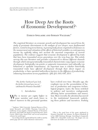
Figure 1 (from Cavalli-Sforza, Menozzi,
and Piazza 1994, page 78) is a phylogenetic
tree illustrating how different human popu-
lations have split apart over time. Such phy-
logenetic trees, constructed from genetic
distance data, are the population analogs
of family trees for individuals. In this tree,
the greatest genetic distance observed is
between Mbuti Pygmies and Papua New
Guineans, where the FST distance is 0.4573,
17 To accommodate the fact that some countries are
composed of different genetic groups (e.g., the United
States), we computed a measure of “weighted genetic
distance,” representing the expected genetic distance
between two randomly chosen individuals, one from each
country, using the genetic distances associated with their
respective ancestor populations. That is, we do not con-
sider the inhabitants of countries composed of different
genetic groups as a new homogeneous “population” in
the biological sense, but treat each of those countries as
formed by distinct populations, to accurately capture the
differences in ancestor-transmitted traits within and across
countries. This is the measure used in the empirical work
discussed below.
and the smallest is between the Danish and
the English, where the genetic distance is
0.0021.18
To properly interpret the effect of genetic
distance on differences in economic out-
comes, two important clarifications are in
order. First, since genetic distance is based
on neutral change, it is not meant to cap-
ture differences in specific genetic traits
that can directly matter for survival and fit-
ness. Hence, we emphasize that empiri-
cal work using genetic distance provides
no evidence for an effect of specific genes
on income or productivity. Evidence of an
“effect of genetic distance” is not evidence
of a “genetic effect.” Rather, it can serve as
evidence for the importance of intergenera-
tionally transmitted traits, including traits
that are transmitted culturally from one gen-
eration to the next.
Second, the mechanism need not be a
direct effect of those traits (whether cultur-
ally or genetically transmitted) on income
and productivity. Rather, divergences in
human traits, habits, norms, etc. have cre-
ated barriers to communication and imita-
tion across societies. While it is possible that
intergenerationally transmitted traits have
direct effects on productivity and economic
performance (for example, if some parents
transmit a stronger work ethic to their chil-
dren), another possibility is that human traits
also act to hinder development through a
barrier effect: more closely related societies
are more likely to learn from each other and
adopt each other’s innovations. It is easier for
someone to learn from a sibling than from
a cousin, and easier to learn from a cousin
18 Among the more disaggregated data for Europe, also
used in Spolaore and Wacziarg (2009), the smallest genetic
distance (equal to 0.0009) is between the Dutch and the
Danish, and the largest (equal to 0.0667) is between the
Lapps and the Sardinians. The mean genetic distance
across European populations is 0.013. Genetic distances
are roughly ten times smaller on average across popula-
tions of Europe than in the world data set.

0.2 0.15 0.1 0.05 0
San (Bushmen)
Mbuti Pygmy
Bantu
Nilotic
W. African
Ethiopian
S.E. Indian
Lapp
Berber, N. African
Sardinian
Indian
S.W. Asian
Iranian
Greek
Basque
Italian
Danish
English
Samoyed
Mongol
Tibetan
Korean
Japanese
Ainu
N. Turkic
Eskimo
Chukchi
S. Amerind
C. Amerind
N. Amerind
N.W. American
S. Chinese
Mon Khmer
Thai
Indonesian
Philippine
Malaysian
Polynesian
Micronesian
Melanesian
New Guinean
Australian
FST
Genetic
Distance
Figure 1. Genetic Distance among Forty-two Populations
Source: Cavalli-Sforza, Menozzi, and Piazza (1994).

than from a stranger. Populations that share
more recent common ancestors have had
less time to diverge in a wide range of traits
and characteristics—many of them cultural
rather than biological—that are transmitted
from a generation to the next with variation.
Similarity in such traits facilitates communi-
cation and learning, and hence the diffusion
and adaptation of complex technological and
institutional innovations.
Under this barriers interpretation, dif-
ferences in traits across populations hinder
the flow of technologies, goods and people,
and in turn these barriers hurt development.
For instance, historically rooted differences
may generate mistrust, miscommunica-
tion, and even racial or ethnic bias and dis-
crimination, hindering interactions between
populations that could result in a quicker
diffusion of productivity-enhancing innova-
tions from the technological frontier to the
rest of the world. The barriers framework in
Spolaore and Wacziarg (2009) predicts that,
ultimately, genetic distance should have no
residual effect on income differences (unless
another major innovation occurs), as more
and more societies, farther from the frontier,
come to imitate the frontier technology. This
is consistent with the diffusion of economic
development as emerging from the forma-
tion of a human web, gradually joined by dif-
ferent cultures and societies in function of
their relative distance from the technological
frontier (McNeill and McNeill 2003).
We test the idea that genealogical relat-
edness facilitates the diffusion of develop-
ment in our unified empirical framework.
Table 7, columns 1 and 2 introduce genetic
distance to the United States in our basic
income level regression, controlling for the
baseline geographic variables.19
Genetic
19 Since several countries in our sample, especially the
technological frontier (the United States) are composed of
several distinct genetic groups, we used a weighted mea-
sure of genetic distance, capturing the expected genetic
distance as of 1500, reflecting the distance
between indigenous populations, is nega-
tively and significantly related to log income
per capita in 2005. The effect rises in mag-
nitude when considering genetic distance to
the United States using the current genetic
composition of countries. In other words,
ancestry-adjusted genetic distance once
more is a better predictor of current income
than a variable based on indigenous charac-
teristics, consistent with the results in table
5. Column 3 of table 7 introduces genetic
distance alongside the share of Europeans,
showing that genetic distance to the United
States bears a significant partial correla-
tion with current income that is not entirely
attributable to the presence of Europeans.
While these simple regressions are infor-
mative, a better test of the hypothesis that
genetic distance captures human barriers
to the diffusion of development relies on a
bilateral approach, whereby absolute log
income differences are regressed on bilat-
eral genetic distance, analogous to a gravity
approach in international trade. This was the
main approach in Spolaore and Wacziarg
(2009), and is reflected in tables 8 and 9. The
bilateral approach offers a test of the barriers
story: if genetic distance acts as a barrier, it
should not be the simple distance between
countries that matters, but their genetic
distance relative to the world technological
frontier. In other words if genetic distance
acts as a barrier, it should not be the genetic
distance between, say, Ecuador and Brazil
that should better explain their income dif-
ference, but their relative genetic distance
to the United States, defined as the absolute
distance between two individuals, randomly selected from
each of the two countries in a pair. Formally, the weighted
FST genetic distance between countries 1 and 2 is defined
as:
FST 12 W
  = ∑ 
i=1
  
I
   ∑ 
j=1
  
J
    ( s1i  × s2 j  × dij )
where skiis the share of group i in country k, dijis the FST
genetic distance between groups i and j.

difference between the Ecuador–U.S.
genetic distance and the Brazil–U.S. genetic
distance.
The specifications we use are as follows:
First, we estimate the effect of simple
weighted genetic distance, denoted FST ij W
,
between country i and country j, on the abso-
lute difference in log per capita income
between the two countries, controlling for a
vector Xijof additional bilateral variables of
a geographic nature:
(1) | log  Yi − log  Yj | = β0 + β1  FST ij W
 
+ β 2 ′   Xij + εij .
Second, we estimate the same specifica-
tion, but using as a regressor relative genetic
Table 7
Genetic Distance and Economic Development, Cross-Sectional Regressions
(Dependent variable: log per capita income, 2005)
Main regressor:
Indigenous
genetic distance
Ancestry-adjusted
genetic distance
Control for the
share of Europeans
(1) (2) (3)
Fstgenetic distance to the United States, –4.038
1500 match (3.846)***
Fstgenetic distance to the United States, –6.440 –4.576
weighted, current match (3.392)*** (2.341)**
Absolute latitude 0.034 0.030 0.015
(5.068)*** (4.216)*** (1.838)*
Percent land area in the tropics –0.182 –0.041 –0.384
(0.582) (0.135) (1.189)
Landlocked dummy –0.637 –0.537 –0.521
(3.686)*** (2.971)*** (3.051)***
Island dummy 0.584 0.607 0.557
(2.389)** (2.392)** (2.262)**
Share of descendants of Europeans, 0.863
per Putterman and Weil (3.601)***
Constant 8.451 8.618 8.637
(23.577)*** (21.563)*** (20.941)***
Beta coefficients on the bold variable –23.85% –27.11% –20.30%
Observations 155 154 149
R2
0.499 0.496 0.545

Table 8
Income Difference Regressions with Genetic Distance
(Dependent variable: absolute value of difference in log per capita income, 2005)
Specification includes: Simple GD Relative GD Horserace
Control for
Europeans Relative GD
Estimator: OLS OLS OLS OLS
2SLS with
1500 GD
(1) (2) (3) (4) (5)
Fstgenetic distance, weighted 2.735 0.607
(0.687)** (0.683)
Fstgen. dist. relative to the 5.971 5.465 5.104 9.406
United States, weighted (1.085)** (1.174)** (1.038)** (1.887)**
Absolute difference in the 0.620
shares of people of
European descent
(0.124)**
Absolute difference in latitudes 0.562 0.217 0.268 –0.369 0.112
(0.277)** (0.242) (0.250) (0.200)* (0.294)
Absolute difference in longitudes –0.117 –0.016 0.024 –0.308 0.245
(0.230) (0.214) (0.205) (0.198) (0.240)
Geodesic distance –0.017 –0.018 –0.025 0.025 –0.049
(0.030) (0.029) (0.028) (0.027) (0.031)
=1 for contiguity –0.536 –0.475 –0.469 –0.351 –0.395
(0.057)** (0.059)** (0.060)** (0.064)** (0.066)**
=1 if either country is an island 0.123 0.143 0.147 0.181 0.180
(0.097) (0.093) (0.094) (0.095)* (0.093)*
=1 if either country is landlocked 0.047 0.040 0.034 0.076 0.011
(0.089) (0.085) (0.087) (0.085) (0.085)
Difference in percent land area 0.156 0.124 0.113 0.182 0.050
in KG tropical climates (0.095)* (0.096) (0.093) (0.092)** (0.100)
=1 if pair shares at least –0.000 –0.027 –0.027 –0.008 –0.050
one sea or ocean (0.076) (0.067) (0.068) (0.066) (0.079)
Freight rate (surface transport) –0.506 –0.127 –0.162 –0.550 0.078
(0.748) (0.835) (0.835) (0.783) (0.674)
Constant 1.211 1.083 1.078 0.984 0.941
(0.161)** (0.169)** (0.171)** (0.170)** (0.169)**
Standardized Beta, absolute
GD (percent)
19.47 4.32
Standardized Beta, relative
GD (percent)
28.57 26.16 24.43 45.01
Standardized Beta, difference
in Europeans (percent)
24.95
R2
0.08 0.11 0.11 0.16 0.10
Notes: All regressions are based on 10,878 observations from 148 countries. Two-way clustered standard errors in
parentheses.

distance rather than simple genetic distance.
Genetic distance relative to the frontier (the
United States) between countries i and j is
defined as: FST ij R
 = | FST i, US W
    − FST j, US W
  | :
(2) |      log  Yi  − log  Yj |  = γ0  + γ1  FST ij R
 
+ γ 3 ′   Xij  + νij .
Third, we conduct a horse race between
FST ij W
and FST ij R
:
(3) | log   Yi − log  Yj | = δ0 + δ1 FST ij R
 
+ δ2 FST ij W
 
+ δ 3 ′  Xij + ζij .
The prediction of the barrier model is
that the effect of FST ij R
should be larger in
magnitude than the effect of FST ij W
(γ1  > β1),
and that FST ij R
should “win out” in a horse
race (δ1  > δ2).
Consistent with this prediction, in table 8,
columns 1 and 2 show that relative genetic
distance enters with a larger magnitude
than simple genetic distance, and column 3
demonstrates that, when both measures
are entered together, relative genetic dis-
tance trumps simple genetic distance. The
magnitude of the effect is substantial, with
a one standard deviation increase in genetic
distance increasing economic distance by
between 25 percent and 30 percent of a
standard deviation in the absolute difference
in log per capita income, depending on the
specification. Column 4 shows once again
that the effect of genetic distance is robust
to including the absolute difference in the
share of Europeans. In other words, genetic
distance accounts for comparative develop-
ment over and above the role played by the
historical advantage of European popula-
tions. Finally, column 5 attempts to control
for the possible endogeneity of post-1500
migrations (as well as possible measurement
error in contemporary genetic distance) by
using genetic distance in 1500 as an instru-
ment for contemporary genetic distance. The
magnitude of the beta coefficient increases
to 45 percent.
Table 9 examines the relationship
between genetic and economic distances
through history, providing further evidence
for the barriers interpretation. Here, we
consider the relative genetic distance to
the English population in a sample going
back to 1820, using Maddison’s data on per
capita income. We continue to control for
a large number of measures of geographic
distance, climatic differences and transpor-
tation costs. Since the availability of data
changes through time, we report both stan-
dardized betas for the full samples and for
the sample common to all dates. Focusing
on the latter for comparability across time,
we see that the magnitude of the effect
of genetic distance is maximal in 1870, in
the wake of the Industrial Revolution. The
effect then declines steadily from the peak
of 16 percent in 1870 to 7.8 percent in 2005.
This pattern provides a further suggestive
test of the barriers model: in the wake of
a big innovation occurring in Northwestern
Europe, relative genetic distance to the
frontier strongly predicts income differ-
ences, but as more and more countries join
the ranks of industrialized countries, the
effect declines. As already mentioned, this
is consistent with a barrier model, which
predicts that, ultimately, unless another
major innovation occurs, relative genetic
distance should have no residual effect on
income differences, as more and more soci-
eties, increasingly distant from the frontier
society, imitate the frontier technology.
Thus, these findings are consistent with our
interpretation of genetic distance as captur-
ing barriers to the long-term diffusion of
development.
What traits are captured by genetic dis-
tance? By its very definition, genetic distance

is a measure of genealogical relatedness
between human populations. It is important
to stress again that while effects of genetic
distance point to the importance of inter-
generational links, they are not evidence of
direct effects of specific genes or genetically
transmitted traits on income or productiv-
ity. Rather, genetic distance captures genea-
logical relations between populations, and
hence differences in traits that are trans-
mitted vertically from one generation to
the next through a variety of mechanisms,
biologically but also culturally, as well as
through the interactions of the two inheri-
tance systems (gene-culture coevolution).
We detail these different mechanisms in the
next section.
4. The Intergenerational Transmission
of Development
4.1 Mechanisms of Intergenerational
Transmission
The empirical literature on geography and
the reversal of fortune and the more recent
contributions on the role of ancestor popula-
tions suggest that, while there is significant
persistence in development, this persistence
is a characteristic of human populations and
not of geographic locations. The work dis-
cussed so far points to a key role for traits
transmitted from one generation to the next
within populations over the long run. In
this section, we provide a general taxonomy
Table 9
Historical Regressions
(Dependent variable: Absolute difference in log per capita income, 1820 to 2005; estimator: OLS)
Income measured as of:
Income
1820
Income
1870
Income
1913
Income
1960
Income
2005
(1) (2) (3) (4) (5)
Relative Fstgenetic distance to the 0.793 1.885 1.918 4.197 4.842
English population, weighted (0.291)** (0.933)** (0.955)** (0.822)** (0.877)**
Observations 990 1,431 1,596 4,005 10,878
Standardized Beta (percent) 14.31 23.06 20.93 31.56 28.50
Standardized Beta (percent),
common samplea
10.98 16.37 15.53 9.00 7.77
R2
0.36 0.30 0.29 0.22 0.23
Notes: All regressions include an intercept term as well as the following geographic control variables: Absolute
difference in latitudes, absolute difference in longitudes, geodesic distance (1000s of km), dummy for contiguity,
dummy if either country is an island, difference in percent land area in KG tropical climates, dummy if either coun-
try is landlocked, dummy if pair shares at least one sea or ocean, freight rate. Two-way clustered standard errors in
parentheses.
a
Common sample of 780 observations based on 40 countries for which data is available across all periods.

of the different channels and mechanisms
through which these traits can be transmit-
ted across generations and affect economic
development. We then use this framework to
discuss recent contributions to the econom-
ics literature.
The starting point for our discussion is
a classification of different mechanisms of
intergenerational transmission. The more
recent literature on heredity and evolution
stresses that inheritance mechanisms are
diverse and cannot be reduced to the old
nature versus nurture dichotomy. On the
contrary, people and societies inherit traits
from their ancestors through a complex
interaction of biological and cultural mecha-
nisms, with an essential role played by envi-
ronmental factors. Following Jablonka and
Lamb (2005), we consider four inheritance
dimensions: genetic, epigenetic, behavioral,
and symbolic. For convenience and to keep
the taxonomy relatively simple, we refer to
the first two dimensions (genetic and epi-
genetic) as “biological” and the remaining
two dimensions (behavioral and symbolic) as
“cultural.”
The genetic dimension has its molecular
basis in DNA and its replication. Modern
genetics stresses that the genome is a com-
plex and dynamic system, and that genes
alone do not determine individual charac-
teristics. For example, Jablonka and Lamb
(2005) write: “The stretch of DNA that is a
‘gene’ has meaning only within the system as
a whole. And because the effect of a gene
depends on its context, very often a change
in a single gene does not have a consistent
effect on the trait that it influences” (7). In
general, it is useful to view genetic transmis-
sion as part of a broader system, interact-
ing with other factors, including our second
dimension: epigenetics.
The epigenetic dimension, even though
important in biology and medicine, is not as
well known among nonspecialists. Epigenetic
inheritance systems refer to the ways cells
withidenticalgeneticinformationcanacquire
different phenotypes and transmit them to
their daughter cells through the inheritance
of epigenetic markers (for example, methyla-
tion patterns). The epigenetic dimension is
vital for the biological development of indi-
vidual organisms. In addition, some scholars
argue that it may play an important role in
evolution over time. An insightful and enter-
taining discussion of this view is provided
in Jablonka and Lamb (2005, chapter 4). As
they explain, “A person’s liver cells, skin cells,
and kidney cells, look different, behave dif-
ferently, and function differently, yet they all
contain the same genetic information. With
very few exceptions, the differences between
specialized cells are epigenetic, not genetic.
They are the consequences of events that
occurred during the developmental history
of each type of cell and determined which
genes are turned on, and how their products
act and interact (. . .). Although their DNA
sequences remain unchanged during devel-
opment, cells nevertheless acquire informa-
tion that they can pass to their progeny. This
information is transmitted through what are
known as epigenetic inheritance systems”
(113). Even though the extent and relevance
of heritable epigenetic effects is debated in
the biological literature, there is increasing
evidence that changes in the epigenome can
be inherited across generations (“paramuta-
tion”). Reviews of the evidence are provided,
for instance, in Chandler and Alleman (2008)
and, for humans, in Morgan and Whitelaw
(2008).20
This mechanism could provide an
explanation for rapid changes in populations
that could not be brought about by genetic
selection. In general, it is conceptually
20 Morgan and Whitelaw (2008) mention the well-
known Dutch Famine Birth Cohort Study (Lumey 1992),
which reported that children born during famine in World
War II were smaller than average and that the effects could
last two generations. However, they also point out that a
subsequent report by Stein and Lumey (2000) failed to
reproduce some of the findings.

appropriate to consider both genetic and
epigenetic transmission, and their interac-
tions, when discussing biological inheritance
systems.21
Clearly, humans do not inherit traits only
biologically from their ancestors. Typically,
people acquire all sorts of traits through
cultural transmission (for example their
mother tongue and all kinds of views and
beliefs about the world). We can distinguish
between behavioral transmission, which
is also common among some animals (for
instance, monkeys), and symbolic transmis-
sion, which some scholars view as uniquely
human—the philosopher Cassirer (1944)
famously defined man as “the symbolic
animal.” Both mechanisms involve social
learning. Behavioral transmission refers to
learning by direct observation and imita-
tion: I learned how to cook spaghetti by
watching my dad in the kitchen. In contrast,
symbolic transmission allows learning via
systems of symbols: I learned how to cook
goulash from a cookbook. Human norms,
habits, values, etc. tend to be passed across
generations both behaviorally (by example)
and symbolically (using language, art, writ-
ing, and so on). In general, culture can be
defined as “information capable of affecting
individuals’ behavior that they acquire from
other members of their species through
teaching, imitation, and other forms of social
transmission” (Richerson and Boyd 2005,
5).22
In their insightful discussion of the
21 In a different context, the relevance of epigenetics
for the study of economic outcomes has been emphasized
in the microeconomic literature on human capital forma-
tion. For instance, Cunha and Heckman (2007) write: “the
nature versus nurture distinction is obsolete. The modern
literature on epigenetic expression teaches us that the
sharp distinction between acquired skills and ability fea-
tured in the early human capital literature is not tenable”
(32).
22 Of course, this is one among many possible defini-
tions of culture. It is well known that the word “culture”
has multiple meanings. In a widely cited study, Kroeber
and Kluckhohn (1952) provided 164 definitions of culture.
“evolution of cultural evolution,” Henrich
and McElreath (2003) write: “While a vari-
ety of local genetic adaptations exist within
our species, it seems certain that the same
basic genetic endowment produces arctic
foraging, tropical horticulture, and desert
pastoralism [. . .]. The behavioral adapta-
tions that explain the immense success of
our species are cultural in the sense that they
are transmitted among individuals by social
learning and have accumulated over gen-
erations. Understanding how and when such
culturally evolved adaptations arise requires
understanding of both the evolution of the
psychological mechanisms that underlie
human social learning and the evolutionary
(population) dynamics of cultural systems”
(123).23
While it is conceptually useful to dis-
tinguish between biological and cultural
transmission, we must keep in mind that in
reality those dimensions are interconnected
in complex ways. An increasingly influential
literature within population genetics has
emphasized that human outcomes often
stem from the interaction of biological and
cultural factors. Both genes and culture are
informational entities that are transmitted at
different rates across generations with varia-
tions, and can be studied within a unified
framework that focuses on the interaction
between biological and cultural inheritance
systems. This approach is known as dual
inheritance theory or gene–culture coevolu-
tion (Cavalli-Sforza and Feldman 1981; Boyd
and Richerson 1985; Richerson and Boyd
2005). In such a framework, individual out-
comes (phenotypes) are a mix of genetically
and culturally transmitted traits, affecting
the transmission rates of different genetic
and cultural information. As Richerson and
Boyd (2005) point out, genes and culture can
23 An interesting example of analysis of cultural evolu-
tion with long-term implications for economic develop-
ment is Shariff, Norenzayan, and Henrich (2010).

be seen as “obligate mutualists, like two spe-
cies that synergistically combine their spe-
cialized capacities to do things that neither
can do alone. [ . . . ] Genes, by themselves
can’t readily adapt to rapidly changing envi-
ronments. Cultural variants, by themselves,
can’t do anything without brains and bodies.
Genes and culture are tightly coupled but
subject to evolutionary forces that tug behav-
ior in different directions” (194).
Proponents of dual inheritance theory
believe that gene–culture evolution has
played an important role in the evolution
of human social psychology, including the
evolution of social norms and institutions
(e.g., Richerson and Boyd, chapter 6). This
view informs a broad literature on the coevo-
lution of preferences, institutions and behav-
ior, such as the analyses of the evolution of
altruistic behavior by Boyd et al. (2003) and
Gintis et al. (2003). General discussions of
the emergence of prosperity-generating
behavior from an evolutionary perspective
are provided by Seabright (2010) and Ridley
(2010).
A famous example of gene–culture coevo-
lution is the evolution of adult tolerance for
milk in some, but not all, human popula-
tions (Simoons 1969, 1970).24
Most people,
like most other mammals, can digest milk as
infants but not as adults, because they lack
the enzyme to digest lactose. However, there
are several populations where most adults
can indeed digest milk. The largest concen-
tration of lactose absorbers can be found in
Northwestern Europe, where less than 10–15
percent of the population is lactose intoler-
ant. Low levels of lactose intolerance are
also found among Indians and some African
populations (Tutsi and Fulani). In contrast,
few Far Easterners, Bantu Africans, Pacific
Islanders, and Native Americans can digest
milk as adults.
24 See also Durham (1991, chapter 5) and Richerson
and Boyd (2005, chapter 6).
It is now well understood that the adult
ability to digest milk evolved in response to
a cultural innovation: dairying. The (domi-
nant) gene controlling lactose absorption
spread rapidly among populations that kept
cows, sheep or goats, making those practices
even more valuable from an evolutionary
perspective. It also spread, but to a lesser
extent, among Mediterranean people who
consume milk in the form of cheese and
yogurt, from which the lactose has been
removed, but it did not spread among popu-
lations without a dairying tradition. To pre-
dict whether a current population would
have a high or low tolerance for milk, one
must look at the history of dairying among
the population’s ancestors, no matter where
they lived, rather than to the history of dairy-
ing in that population’s current territory.
For instance, within the United States, it
has been observed that the percentage of
lactose intolerant adults is almost 100 per-
cent among Native Americans, 90 percent
among Asian Americans, 75 percent among
African Americans, and only 12 percent
among European Americans (Kretchmer
1972; Enattah et al. 2002). This is consistent
with the intergenerational transmission of
the lactose absorption trait over an extended
historical span, through genetic and cultural
interaction.25
In general, the economic effects of human
characteristics are likely to result from inter-
actions of biological and cultural factors, with
the effects of genetic or epigenetic charac-
teristics on economic outcomes changing
over space and time depending on cultural
characteristics, and vice versa. Consider,
for example, differences across individuals
within a given population (say, the United
States) with respect to a clearly genetic fea-
ture, such as having two X chromosomes,
the purely genetic characteristic associated
25 More examples of gene–culture interaction, and a
taxonomy, are provided by Durham (1991).

with the female gender. This characteristic
is likely to have had very different effects
on a person’s income, life expectancy, and
other outcomes in the year 1900 and in the
year 2000, because of changes in culturally
transmitted characteristics over the century.
This is a case where the impact of genes on
outcomes varies with a change in cultural
characteristics.26
Conversely, we can think
of the differential impact of a given cultural
characteristic—for example, the habit of
drinking alcohol—on individuals with differ-
ent genetic traits, such as variation in alcohol
dehydrogenase, the alcohol-metabolizing
enzyme.
In sum, we can aggregate inheritance
dimensions and their complex interactions in
three broad sets: (a) biological transmission
(genetic and epigenetic, and their interac-
tion), (b) cultural transmission (behavioral
and symbolic, and their interaction), and (c)
dual, capturing the interactions between bio-
logical and cultural transmission.
4.2 Direct and Barrier Effects
When considering how traits transmit-
ted along these different channels may have
affected development, we must introduce an
additional distinction, orthogonal to the cat-
egories discussed up to this point. No mat-
ter how traits are transmitted, their effects
on economic performance might operate
either directly or as barriers to the diffusion
of development.
One possibility is that intergeneration-
ally transmitted traits have direct effects on
productivity and economic performance.
A slow-changing cultural trait developed
in early history could be conducive directly
to high incomes in modern times if it is
26 This is a variation on an example by Alison Gopnik
in her comment to debate between Steven Pinker and
Elizabeth Spelke at http://www.edge.org/discourse/
science-gender.html#ag. Steven Pinker’s response is also
available at http://www.edge.org/discourse/sciencegender.
html.
transmitted from parents to kids within
populations, either behaviorally or through
complex symbolic systems (e.g., by religious
teaching). For example, a direct effect stem-
ming from cultural transmission would be
Weber’s (1905) argument that the Protestant
ethic was a causal factor in industrializa-
tion (a recent critical reassessment of this
hypothesis has been provided by Becker and
Woessmann 2009).
As we discussed in the previous section,
another possibility is that human traits act to
hinder development through a barrier effect.
In this case, it is not the trait itself that directly
affects economic performance. Rather, it
is differences in inherited characteristics
across populations that create barriers to the
flow of technological and institutional inno-
vations, ideas, etc., and, consequently, hurt
development. Historically rooted differences
may generate barriers—e.g., via cultural,
racial, and ethnic bias, discrimination, mis-
trust, and miscommunication—hindering
interactions between populations that could
result in a quicker diffusion of productivity-
enhancing innovations across populations, as
in Spolaore and Wacziarg (2009). A focus on
barriers can explain why differences in inher-
ited traits may matter, even though many
new ideas and innovations are learned “hori-
zontally” from individuals and populations
that are not directly related, rather than “ver-
tically” from one’s close relatives and ances-
tors. The fact is that, when barrier effects
exist, vertically transmitted traits also affect
horizontal learning and diffusion. People are
more likely to learn new ideas and adopt new
technologies from other people who, while
not directly related to them, share more
recent common ancestors and, consequently,
on average, a larger set of inherited traits and
characteristics.
The microeconomic literature on the dif-
fusion of innovations (Rogers 2003) is consis-
tent with a major role for subjective barriers
between groups and populations. As Rogers

points out, summarizing the lessons from
decades of research, most people depend
upon a subjective evaluation of an innovation
that is conveyed to them from other indi-
viduals like themselves, who have previously
adopted the innovation. This dependence on
the experience of near peers suggests that,
at the heart of the diffusion process, we can
often find potential adopters’ imitation of
their network partners.
4.3 A General Taxonomy
The distinction between barrier effects
and direct effects on the one hand, and the
different forms of intergenerational trans-
mission on the other hand, can be conve-
niently captured in the following matrix:
Direct
Effect
Barrier
Effect
Biological Transmission
Quadrant I Quadrant IV(genetic and/or
epigenetic)
Cultural Transmission
Quadrant II Quadrant V(behavioral and/or
symbolic)
Dual Transmission
Quadrant III Quadrant VI(biological-cultural
interaction)
In what follows, we provide examples of
each of these quadrants from contributions
to the social sciences, with a particular focus
on research that stresses the role of intergen-
erationally transmitted traits on economic
development. As we will see, mechanisms
from all six of the quadrants in the figure
above have been studied in the economic
literature. However, so far there have been
no systematic attempt to quantify the respec-
tive power of each of the major explanations,
nor has there been enough work on the pre-
cise traits that can account for either direct
or barrier effects on development. These
are the major avenues for promising future
research in this emerging field.
In light of the advances in the scientific
literature that we have mentioned above,
which have emphasized the interconnection
and coevolution of biological and cultural
traits, it may be very hard, or even mean-
ingless, to separate biological and cultural
effects in the long run. Therefore, while the
rows in our taxonomy matrix provide useful
ideal benchmarks from a theoretical perspec-
tive, a more productive empirical approach
might be to focus on whether such intergen-
erational mechanisms—whether biological
or cultural (or dual)—operate directly or as
barriers to the diffusion of technological and
institutional innovations—i.e., to identify
the respective roles of each column rather
than each row in the matrix that summarizes
our proposed taxonomy. We return to these
points below, as we discuss specific contribu-
tions to the economic literature.
4.3.1 Quadrants I, II, and III
A theory of development centered on a
direct effect of biologically transmitted char-
acteristics (Quadrant I) is provided in Galor
and Moav (2002). These authors suggest that
there may exist an intergenerationally trans-
mitted trait affecting humans’ fertility strate-
gies, with some individuals inheriting traits
that induce them to follow a quantity-biased
strategy (having a high number of children),
while others would lean toward quality-
biased strategies (high parental investment
in a smaller number of children).27
Galor and
Moav (2002) then argue that the evolution-
ary dynamics of these traits had important
implications for the onset of the Industrial
Revolution and the following demographic
transition. Their starting point is the pre-
industrial world, where everybody was
27 The authors are careful to notice that such differ-
ences do not imply that one strategy is “better” than the
other, in the same way as we cannot say that giant sequoias
(which follow an extreme quality-biased strategy) are “bet-
ter” than humans.

Economic roots (1)

Recommended

Recommended

More Related Content

What's hot

What's hot (20)

Viewers also liked

Viewers also liked (15)

Similar to Economic roots (1)

Similar to Economic roots (1) (20)

Recently uploaded

Recently uploaded (20)

Economic roots (1)