This document summarizes a digital signal processing project that involves resampling audio signals and modeling signals using autoregressive (AR) processes.
The resampling part involves downsampling two audio signals with correct and incorrect sampling rate conversions. Graphs and analysis show the resampled signals have lower quality and more distortion compared to the originals.
The AR modeling part estimates AR model coefficients from one of the signals using the Yule-Walker equations. A filter is designed to "whiten" the signal, removing noise. Graphs and audio comparison show the filtered signal has less noise but also some quality loss.
Modified freeform offner, august 11, 2021Dave Shafer
An Offner 1.0X relay system can be given a greatly increased field size with good aberration correction by adding to the design two 45 degree flat fold mirrors that are given some freeform aspheric deformation.
Professor Mark Beach's presentation (without videos) on the University of Bristol's Massive MIMO activities as given at the IET's 'Towards 5G Mobile Technology – Vision to Reality' event, January 25th 2017.
A survey of some interesting Gregorian telescope designs includes some with all spherical surfaces as well as some with a 20 meter spherical f/1.0 primary mirror and sub-aperture corrector mirrors.
what is gifi?
GIFI stands for General Index of Financial Information.
The GIFI is a system that assigns a unique code to a list of items commonly found on income statements, balance sheets, and statements of earnings.
The purpose of the GIFI is to allow the CRA (Canada Revenue Agency) to collect and process financial information more efficiently. For instance, the GIFI lets the CRA validate tax table information electronically rather than manually.
The application wavelet transform algorithm in testing adc effective number o...ijcsit
In evaluating Analog to Digital Convertors, many parameters are checked for performance and error rate.
One of these parameters is the device Effective Number of Bits. In classical testing of Effective Number of
Bits, testing is based on signal to noise components ratio (SNR), whose coefficients are driven via
frequency domain (Fourier Transform) of ADC’s output signal. Such a technique is extremely sensitive to
noise and require large number of data samples. That is, longer and more complex testing process as the
device under test increases in resolutions. Meanwhile, a new time – frequency domain approach (known as
Wavelet transform) is proposed to measure and analyze Analog-to-Digital Converters parameter of
Effective Number of Bits with less complexity and fewer data samples.
Phase locked loop is a technique usually used to perform indirect digital frequency synthesizer for
most RF transceivers. A fractional-N phase locked loop frequency synthesizer has been used in recent years
since it achieves fine resolution and large loop bandwidth . This paper presents the design and simulation of a
fractional-N phase locked loop frequency synthesizer using sigma-delta modulation for bluetooth standard
systems with a frequency range from 2402 to 2480MHz. Loop filter and Sigma-Delta modulator are the most
important factors in improving the performance of fractional-N phase locked loop. The digital Sigma-Delta
modulator provides a useful noise shaping for the phase noise introduced by the fractional division operation,
while the loop filter bandwidth limits the speed of switching time between the synthesized frequencies. A forth
order passive loop filter was implemented at bandwidth equal to 200 KHz, 50° phase margin, and a second
order single loop modulator with 4-level quantizer was used to control the frequency divider. Simulation results
showed that the system is stable, and there is no fractional spurs in the output spectrum of the fractional-N
phase locked loop.
FPGA Design & Simulation Modeling of Baseband Data Transmission SystemIOSR Journals
Abstract: This paper describes a study on a baseband data transmission system developed for undergraduate
students studying communication engineering. Theoretical material, developed in the lectures, is briefly
covered. A practical system is presented with pre-detection filtering being employed to improve the bit error
rate. A simulation of the complete system is carried out on a Sun work station using the MATLAB simulation
package. Simulation and theoretical results are compared.
IJRET : International Journal of Research in Engineering and Technology is an international peer reviewed, online journal published by eSAT Publishing House for the enhancement of research in various disciplines of Engineering and Technology. The aim and scope of the journal is to provide an academic medium and an important reference for the advancement and dissemination of research results that support high-level learning, teaching and research in the fields of Engineering and Technology. We bring together Scientists, Academician, Field Engineers, Scholars and Students of related fields of Engineering and Technology
Performance analysis of new proposed window for the improvement of snr & ...eSAT Journals
Abstract
The process of communication becomes quite challenging because of the unwanted electrical signals in a communications system. These undesirable signals, usually termed as noise, are random in nature and interfere with the message signals. As a result the signal which is collected from receiver side is not accurate level .In this respects, filtering of signal is very important because noisy signal can mask some important features of the message signal. Hence it is desirable to reduce this noise for proper analysis of the message signal. The signal to noise ratio (SNR) is one of the important measures for reducing the noise. This paper presents the study of low pass FIR filter using a new window techniques for signal Processing. The newly designed windowing filterpresents a new concept for better signal analysis and disturbance detection in the communication systems.The parameters i.e. Power Spectral Density (PSD), signal to noise ratio (SNR), Error Vector Magnitude (EVM) & Figure of Merit are calculated of original signal and analysis the performance of new proposed window method used for low pass FIR filter. This new windowing filter finds applications in signal analysis, communication system and image compression with a lot of other fields.The results have been concluded using MATLAB R2012 software. Index Terms:Window method for Noise reduction, Figure of Merit, SNR, EVM, New window performance
Computer aided design of communication systems / Simulation Communication Sys...Makan Mohammadi
The report introduces how to use computer simulation in the design of physical layer transmission protocols that are too complex for a purely analytical approach. The goal of the report is to offer the theoretical and practical tools for performing modeling, analysis, and design of the physical level of wireless transmission systems including cellular and personal communication systems, satellite systems and radio relay links. This course is useful for telecommunication systems designers, ICT researchers and experts in the development and design of telecommunication physical layer protocols.
Design of 17-Bit Audio Band Delta-Sigma Analog to Digital ConverterKarthik Rathinavel
• Systematically designed a delta sigma ADC with CIFF modular architecture in MATLAB Simulink with an ENOB of 19-bits.
• Designed a decimation filter to remove noise in the digital output of the delta sigma modulator.
• Observed the effect of non-idealities on the modulator such as finite gain, finite bandwidth, slew rate, analog noise and capacitor mismatch.
Designed a Switched Capacitor Low Pass Filter with a sampling frequency of 60 Hz.
Simulated the filter to have a ripple within 0.2 dB under 3.6 MHz and a stopband attenuation of atleast -51 dB after 7.2 MHz.
Applied dynamic range optimization, Dynamic Range Scaling and Chip Area scaling to get maximum output swing while occupying minimum area on chip.
Tested the filter with non-idealities of the amplifier, such as finite gain, bandwidth, offset voltage, charge injection, etc.
DESIGN REALIZATION AND PERFORMANCE EVALUATION OF AN ACOUSTIC ECHO CANCELLATIO...sipij
Nowadays, in the field of communications, AEC (acoustic echo cancellation) is truly essential with respect
to the quality of multimedia transmission. In this paper, we designed and developed an efficient AEC based
on adaptive filters to improve quality of service in telecommunications against the phenomena of acoustic
echo, which is indeed a problem in hands-free communications.The main advantage of the proposed algorithm is its capacity of tracking non-stationary signals such as acoustic echo. In this work the acoustic echo cancellation (AEC) is modeled using a digital signal
processing technique especially Simulink Blocksets. The algorithm’s code is generated in Matlab Simulink
programming environment. At simulation level, results of simulink implementation prove that module
behavior is realistic when it comes to cancellation of echo in hands free communication using adaptive algorithm.Results obtained with our algorithm in terms of ERLE criteria are confronted to IUT-T recommendation
G.168.
Noise reduction is the process of removing noise from a signal. In this project, two audio files are given: (1) speech.au and (2) noisy_speech.au. The first file contains the original speech signal and the second one contains the noisy version of the first signal. The objective of this project is to reduce the noise from the noisy file
Echo and reverberation effects are used extensively in the music industry. Here we will design a digital filter that will create the echo and reverb effect on audio signals.
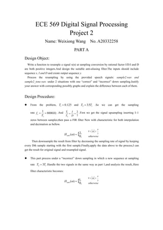
1. ECE 569 Digital Signal Processing
Project 2
Name: Weixiong Wang No. A20332258
PART A
Design Object:
Write a function to resample a signal x(n) at sampling conversion by rational factor I/D.I and D
are both positive integers.And design the suitable anti-aliasing filter.The inputs should include
sequence x, I and D and create output sequence y.
Process the resampling by using the provided speech signals: sample2.wav and
sample2_tone.wav. under 2 situations with one “correct” and “incorrect” down sampling.Justify
your answer with corresponding possibly graphs and explain the difference between each of them.
Design Procedure:
From the problem, 125.01 T and 12 53 T.T .So we can get the sampling
rate Hz
T
fs 8000
1
1
.And
7
2
2
1
D
I
T
T .First we get the signal upsampling inserting I–1
zeros between samples;then pass a FIR filter New with characteristic for both interpolation
and decimation as bellow.
7
0
,2
,0
)( {
otherwiseantiH
Then downsample the result from filter by decreasing the sampling rate of signal by keeping
every Dth sample starting with the first sample.Finally,apply the data above to the process,I can
get the result for original signal and resampled signal.
This part process under a “incorrect” down sampling in which a new sequence at sampling
rate 12 3TT .Handle the two signals in the same way as part 1,and analysis the result,.Here
filter characteristic becomes:
3
0
,1
,0
)( {
otherwiseantiH
2. Design Result:
Below are the results of resampling process in ‘correct’ down sampling,red line represent
origin signal and green line represent resampled signal.As shown in the Figure A.1.1,for the
sample2.wav.After resampling,the resampled signal becomes vague compared to the original
signal,which can be reflected from the figure A.1.1.We can see the loss of quality for signal.
0 0.5 1 1.5 2 2.5
-0.8
-0.6
-0.4
-0.2
0
0.2
0.4
0.6
0.8
1
Time(second)
WaveMagnitude
origin
resampled
Figure A.1.1
As for the sample2_tone.wav.Resampling get away the noise and preserve the useful signal to a
certain extent.But the audio performance is a little worse than the first resampled signal,which
means there are more loss during the resampling process,because of the noise,reflected on rhe
figure A.1.2
0 0.5 1 1.5 2 2.5
-1
-0.8
-0.6
-0.4
-0.2
0
0.2
0.4
0.6
0.8
1
Time(second)
WaveMagnitude
origin
resampled
Figure A.1.2
3. Figure A.1.3 is the frequency response comparison between resampled sample2.wav and
sample2_tone.wave.We see that the sample2_tone distorted more than the sample2,which further
illustrate the worse performance of the resampled sample2_tone.
0 0.1 0.2 0.3 0.4 0.5 0.6 0.7 0.8 0.9 1
-50
-40
-30
-20
-10
0
10
20
Normalized frequency ( rad/sample)
Magnitude
Comparison of frequency response of two resampled signals
sample2
sample2tone
Figure A.1.3
This part denote the ‘incorrect’ down sampling,in here 12 3TT ,this method change the
passband of combined filter become broader than the first one.Figure A.2.1 denotes the
sample2.wav and Figure A.2.2 denotes the sample2_tone.wav. Here we can also find the loss
of quality after resampling.
0 0.5 1 1.5 2 2.5
-0.8
-0.6
-0.4
-0.2
0
0.2
0.4
0.6
0.8
1
Time(second)
WaveMagnitude
origin
resampled
Figure A.2.1
4. And the audio difference is similar to the first part.We can still discern the what the audio said
but it will not that clear,resampling loss and the noise disturb made this happen.
0 0.5 1 1.5 2 2.5
-1
-0.8
-0.6
-0.4
-0.2
0
0.2
0.4
0.6
0.8
1
Time(second)
WaveMagnitude origin
resampled
Figure A.2.2
0 0.5 1 1.5 2 2.5
-0.6
-0.4
-0.2
0
0.2
0.4
0.6
0.8
Time(second)
SignalMagnitude
correct
incorrect
Figure A.2.3
Figure A.2.3 denotes the difference of sample2.wav under two different sampling rate
conversion.We can find that in ‘correct’ down sampling the signal approximately envelope the
‘incorrect’ signal.Which is more close to original signal.And the audio of ‘incorrect’ is a little
vague than the ‘correct’ one,which reflected in the Figure A.2.4.
5. Here blue line denotes the original signal,green line denotes correct,red line denotes incorrect.
0 0.1 0.2 0.3 0.4 0.5 0.6 0.7 0.8 0.9 1
-50
-40
-30
-20
-10
0
10
20
30
Normalized frequency ( rad/sample)
Magnitude
Comparison of frequency response of two resampled signals
sample2 correct
original signal
0 0.1 0.2 0.3 0.4 0.5 0.6 0.7 0.8 0.9 1
-40
-30
-20
-10
0
10
20
30
Normalized frequency ( rad/sample)
Magnitude
Comparison of frequency response of two resampled signals
sample2 incorrect
original signal
Figure A.2.4
The signal in correct oscillate less than incorrect one,which more accordant to the original one.
Conclusion for part A:
Resampling applies an anti-aliasing (lowpass) FIR filter to the input signal during the
resampling.This causes some errors, including quality loss in the time domain, and some
frequency domain distortions (since the frequency characteristics of these filters is inperfect).
And we can try to improve the sampling rate to make the reconstructed signal performs better,if
we make the sampling rate ratio equal to 1,then we can reconstruct the audio better than the other
cases.
PART B
Design Object:
This part we want to perform the estimation auto-regressive(AR) process signal model by using
the Yule-Walker equations to get the desired model coefficients A.
Then using the sample2_tone.wav to pass a ‘whiten’ filter to obtain )(nw ,and explain the audio
difference between )(nx and )(nw by suitable graphs.
Design Procedure:
Model coefficients estimation: To solve Yule-Walker equations, we has to know the model
order.Although the Yule-Walker equations can be used to find the model parameters, it cannot
give any insight into the model order N. So we use different order N from small to large to
meet a N that can make the error(noise variance) don’t change significantly when increasing
the order and also the model parameter of the AR process is not-significantly different from
zero.
6. Whiten process: Whitening can be done by filtering with a transfer function that is roughly
the inverse of the power spectrum of the signal.It is an attempt to make the spectrum of the
signal "more uniform".
Design Result:
The estimated model parameters and the noise variances computed by the Yule-Walker
system are given below. It can be ascertained that the estimated parameters are approximately
same as that of what is expected. See how the error decreases as the model order N increases.
The optimum model order in this case is N=7 since the error has not changed significantly
when increasing the order and also the model parameter a7 of the AR(7) process is
not-significantly different from zero.
Below table B.1.1 shows the result.
Model Order(N) Estimated Model
Parameters( ka )
Prediction error
or noise variance(p)
2 [1.0000 -0.0204 0.9804] 0.0061
3 [1.0000 -0.8275 0.9972
-0.8232]
0.0020
4 [1.0000 -1.0420 1.2571
-1.0389 0.2606]
0.0018
5 [1.0000 -0.8954 0.6727
-0.3317 -0.3256 0.5626]
0.0013
6 [1.0000 -0.8007 0.6178
-0.3876 -0.2123 0.4117
0.1684]
0.0012
7 [1.0000 -0.8258 0.5565
-0.3560 -0.1546 0.3197
0.2877 -0.1490]
0.0012
8 [1.0000 -0.8272 0.5592
-0.3530 -0.1560 0.3164
0.2929 -0.1567 0.0094 ]
0.0012
Table B.1.1
In figure B.2.1.The signal after ‘whiten’ wipe out the noise part and leave the useful part.So
when we listen to the audio after ‘whiten’,we can find that the noise disappear,and we can
identify the noise clearly.But the quality loss can also reflected from the figure because of the
noise and delay of filter.
7. 0 0.2 0.4 0.6 0.8 1 1.2 1.4 1.6 1.8 2
x 10
4
-1
-0.5
0
0.5
1
Tone signal
Frequency
Value
0 0.2 0.4 0.6 0.8 1 1.2 1.4 1.6 1.8 2
x 10
4
-0.5
0
0.5
1
Recovered signal
Frequency
Value
Figure B.2.1
The Power Spectral Density associated with N=7 looks very similar to that the 6th order model
because of the similar coefficients and errors,which we can find in the Figure B.2.2 and we can
see the height of the peak is slightly different,but all of them are sensetive but that determined by
how close the poles of the system are to the unit circle.
0 0.1 0.2 0.3 0.4 0.5 0.6 0.7 0.8 0.9 1
-80
-60
-40
-20
0
20
40
Normalized frequency ( rad/sample)
PSD(dB/rad/sample)
Periodogram Power Spectral Density Estimate
PSD estimate of wave
PSD of model output N=2
PSD of model output N=3
PSD of model output N=4
PSD of model output N=5
PSD of model output N=6
PSD of model output N=7
Figure B.2.2
8. So the Yule-Walker equations give us relationships between autocorrelation and autocovariance
of the process and the AR procsee model parameters that give data can be used to obtain
estimation of an AR model for that particular data like we did here.
Conclusion for part B:
A white noise model is appropriate for the speech signal.Because when we filter it,we can get a
good signal.And because the white noise has a more uniform quality.it’s a wide sense stationary
process.We can get the voice by using the autoregressive modeling to a good enough extent.And
an alternative way to do I think ARMA is a good way to realize it,for we can use AR process to
determine the coefficients and variance first and then using MA model to move out the noise in
the tone signal.
Appendix:
Part A.(Resample)
‘Correct’ way
I = 2;
D = 7;
fs=8000;
f = [0 1/7 1/7 1];
m = [2 2 0 0];
h = fir2(50,f,m)
hd = dfilt.dffir(h)
[wave,fs]=wavread('sample2.wav');
sound(wave,fs);
t1=0:1/fs:(length(wave)-1)/fs;
y1 = upsample(wave,I);
y2 = filter(hd,y1);
y3 = downsample(y2,D)
sound(y3,fs*I/D);
t2=(0:(length(y3)-1))*D/(I*fs);
plot(t1,wave,'r',t2,y3,'-g')
xlabel('Time(second)')
ylabel('Wave Magnitude')
legend('origin','resampled')
‘Incorrect’ way
I = 1;
D = 3;
fs=8000;
f = [0 1/3 1/3 1];
m = [1 1 0 0];
h = fir2(50,f,m)
hd = dfilt.dffir(h)
9. [wave,fs]=wavread('sample2.wav');
sound(wave,fs);
t1=0:1/fs:(length(wave)-1)/fs;
y1 = upsample(wave,I);
y2 = filter(hd,y1);
y3 = downsample(y2,D)
sound(y3,fs*I/D);
t2=(0:(length(y3)-1))*D/(I*fs);
plot(t1,wave,'r',t2,y3,'-g')
xlabel('Time(second)')
ylabel('Wave Magnitude')
legend('origin','resampled')
Comparison for each two signal to original signal.
I1 = 2;
D1 = 7;
fs=8000;
f1 = [0 1/7 1/7 1];
m1 = [2 2 0 0];
h1 = fir2(50,f1,m1)
[wave,fs]=wavread('sample2.wav');
y1 = upfirdn(wave,h1,I1,D1);
[H1,w1]=freqz(y1);
[H3,w3]=freqz(wave);
plot(w1/pi,20*log10(2*abs(H1)/(2*pi)),'g-',w3/pi,20*log10(2*abs(H3)/(
2*pi)),'b-')
xlabel('Normalized frequency (times pi rad/sample)');
ylabel('Magnitude');
legend('sample2 correct','original signal')
title('Comparison of frequency response of two resampled signals')
Part B
fs=8000
[wave,fs]=wavread('sample2_tone.wav')
[a,e] = aryule(wave,7)
w=filter(a,1,wave)
sound(w,fs);
subplot(211)
plot(wave)
title('Tone signal');
xlabel('Frequency')
ylabel('Value');
subplot(212)
plot(w)
title('Recovered signal');
xlabel('Frequency')
10. ylabel('Value');
figure(2);
periodogram(wave); hold on; %plot the original frequency response of the
data
N=[2,3,4,5,6,7,8];
set(0,'DefaultAxesColorOrder',[0 0 1;0 1 0;0 1 1;1 0 0;1 0 1;1 1 0;])
for i=1:7,
[a,e] = aryule(wave,N(i))
[H,w]=freqz(sqrt(e),a);
hp = plot(w/pi,20*log10(2*abs(H)/(2*pi))); %plotting in log scale
hold all
end
xlabel('Normalized frequency (times pi rad/sample)');
ylabel('PSD (dB/rad/sample)');
legend('PSD of model output N=2','PSD of model output N=3','PSD of model
output N=4','PSD of model output N=5','PSD of model output N=6','PSD of
model output N=7','PSD of model output N=8');