dynamic programming dp

1. Dynamic Programming

2. 2
DP - Two key ingredients
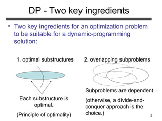
• Two key ingredients for an optimization problem
to be suitable for a dynamic-programming
solution:
Each substructure is
optimal.
(Principle of optimality)
1. optimal substructures 2. overlapping subproblems
Subproblems are dependent.
(otherwise, a divide-and-
conquer approach is the
choice.)

3. 3
Three basic components
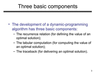
• The development of a dynamic-programming
algorithm has three basic components:
– The recurrence relation (for defining the value of an
optimal solution);
– The tabular computation (for computing the value of
an optimal solution);
– The traceback (for delivering an optimal solution).

4. 4
Dynamic Programming Algorithm
1. Characterize the structure of an optimal
solution
2. Recursively define the value of an optimal
solution
3. Compute the value of an optimal solution in a
bottom-up fashion
4. Construct an optimal solution from computed
information

5. 5
Longest Common Subsequence (LCS)
Application: comparison of two DNA strings
Ex: X= {A B C B D A B }, Y= {B D C A B A}
Longest Common Subsequence:
X = A B C B D A B
Y = B D C A B A
Brute force algorithm would compare each
subsequence of X with the symbols in Y

6. 6
Longest Common Subsequence
• Given two sequences
X = x1, x2, …, xm
Y = y1, y2, …, yn
find a maximum length common subsequence
(LCS) of X and Y
• E.g.:
X = A, B, C, B, D, A, B
• Subsequences of X:
– A subset of elements in the sequence taken in order
A, B, D, B, C, D, B, etc.

7. 7
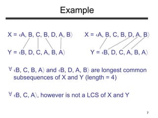
Example
X = A, B, C, B, D, A, B X = A, B, C, B, D, A, B
Y = B, D, C, A, B, A Y = B, D, C, A, B, A
 B, C, B, A and B, D, A, B are longest common
subsequences of X and Y (length = 4)
 B, C, A, however is not a LCS of X and Y

8. 8
Brute-Force Solution
• For every subsequence of X, check whether it’s
a subsequence of Y
• There are 2m
subsequences of X to check
• Each subsequence takes (n) time to check
– scan Y for first letter, from there scan for second, and
so on
• Running time: (n2m
)

9. 9
LCS Algorithm
• First we’ll find the length of LCS. Later we’ll modify
the algorithm to find LCS itself.
• Define Xi, Yj to be the prefixes of X and Y of length i
and j respectively
• Define c[i,j] to be the length of LCS of Xi and Yj
• Then the length of LCS of X and Y will be c[m,n]










otherwise
])
,
1
[
],
1
,
[
max(
],
[
]
[
if
1
]
1
,
1
[
]
,
[
j
i
c
j
i
c
j
y
i
x
j
i
c
j
i
c

10. 10
LCS recursive solution
• We start with i = j = 0 (empty substrings of x and y)
• Since X0 and Y0 are empty strings, their LCS is
always empty (i.e. c[0,0] = 0)
• LCS of empty string and any other string is empty,
so for every i and j: c[0, j] = c[i,0] = 0










otherwise
])
,
1
[
],
1
,
[
max(
],
[
]
[
if
1
]
1
,
1
[
]
,
[
j
i
c
j
i
c
j
y
i
x
j
i
c
j
i
c

11. 11
LCS recursive solution
• When we calculate c[i,j], we consider two cases:
• First case: x[i]=y[j]:
– one more symbol in strings X and Y matches, so the length
of LCS Xi and Yj equals to the length of LCS of smaller
strings Xi-1 and Yi-1 , plus 1










otherwise
])
,
1
[
],
1
,
[
max(
],
[
]
[
if
1
]
1
,
1
[
]
,
[
j
i
c
j
i
c
j
y
i
x
j
i
c
j
i
c

12. 12
LCS recursive solution
• Second case: x[i] != y[j]
– As symbols don’t match, our solution is not improved, and
the length of LCS(Xi , Yj) is the same as before (i.e.
maximum of LCS(Xi, Yj-1) and LCS(Xi-1,Yj)










otherwise
])
,
1
[
],
1
,
[
max(
],
[
]
[
if
1
]
1
,
1
[
]
,
[
j
i
c
j
i
c
j
y
i
x
j
i
c
j
i
c
Why not just take the length of LCS(Xi-1, Yj-1) ?

13. 13
3. Computing the Length of the LCS
0 if i = 0 or j = 0
c[i, j] = c[i-1, j-1] + 1 if xi = yj
max(c[i, j-1], c[i-1, j]) if xi  yj
0 0 0 0 0 0
0
0
0
0
0
yj:
xm
y1 y2 yn
x1
x2
xi
j
i
0 1 2 n
m
1
2
0
first
second

14. 14
Additional Information
0 if i,j = 0
c[i, j] = c[i-1, j-1] + 1 if xi = yj
max(c[i, j-1], c[i-1, j]) if xi  yj
0 0 0 0 0 0
0
0
0
0
0
yj:
D
A C F
A
B
xi
j
i
0 1 2 n
m
1
2
0
A matrix b[i, j]:
• For a subproblem [i, j] it
tells us what choice was
made to obtain the
optimal value
• If xi = yj
b[i, j] = “ ”
• Else, if
c[i - 1, j] ≥ c[i, j-1]
b[i, j] = “  ”
else
b[i, j] = “  ”
3
3 C
D
b & c:
c[i,j-1]
c[i-1,j]

15. 15
LCS-LENGTH(X, Y, m, n)
1. for i 1
← to m
2. do c[i, 0] 0
←
3. for j 0
← to n
4. do c[0, j] 0
←
5. for i 1
← to m
6. do for j 1
← to n
7. do if xi = yj
8. then c[i, j] c[i - 1, j - 1] + 1
←
9. b[i, j ] “ ”
←
10. else if c[i - 1, j] ≥ c[i, j - 1]
11. then c[i, j] c[i - 1, j]
←
12. b[i, j] “ ”
← ↑
13. else c[i, j] c[i, j - 1]
←
14. b[i, j] “ ”
← ←
15.return c and b
The length of the LCS if one of the sequences
is empty is zero
Case 1: xi = yj
Case 2: xi  yj
Running time: (mn)

16. 16
Example
X = A, B, C, B, D, A
Y = B, D, C, A, B, A
0 if i = 0 or j = 0
c[i, j] = c[i-1, j-1] + 1 if xi = yj
max(c[i, j-1], c[i-1, j]) if xi  yj
0 1 2 6
3 4 5
yj B D A
C A B
5
1
2
0
3
4
6
7
D
A
B
xi
C
B
A
B
0 0 0
0 0 0
0
0
0
0
0
0
0
0

0

0

0 1 1 1
1 1 1

1 2 2

1

1 2 2

2

2
1

1

2

2 3 3

1 2

2

2

3

3

1

2

3

2 3 4
1

2

2

3 4

4
If xi = yj
b[i, j] = “ ”
Else if c[i -
1, j] ≥ c[i, j-1]
b[i, j] = “  ”
else
b[i, j] = “  ”

17. 17
4. Constructing a LCS
• Start at b[m, n] and follow the arrows
• When we encounter a “ “ in b[i, j]  xi = yj is an element
of the LCS 0 1 2 6
3 4 5
yj B D A
C A B
5
1
2
0
3
4
6
7
D
A
B
xi
C
B
A
B
0 0 0
0 0 0
0
0
0
0
0
0
0
0

0

0

0 1 1 1
1 1 1

1 2 2

1

1 2 2

2

2
1

1

2

2 3 3

1 2

2

2

3

3

1

2

3

2 3 4
1

2

2

3 4

4

18. 18
PRINT-LCS(b, X, i, j)
1. if i = 0 or j = 0
2. then return
3. if b[i, j] = “ ”
4. then PRINT-LCS(b, X, i - 1, j - 1)
5. print xi
6. elseif b[i, j] = “ ”
↑
7. then PRINT-LCS(b, X, i - 1, j)
8. else PRINT-LCS(b, X, i, j - 1)
Initial call: PRINT-LCS(b, X, length[X], length[Y])
Running time: (m + n)

19. 19
Improving the Code
• If we only need the length of the LCS
– LCS-LENGTH works only on two rows of c at a time
• The row being computed and the previous row
– We can reduce the asymptotic space requirements by
storing only these two rows

20. 20
LCS Algorithm Running Time
• LCS algorithm calculates the values of each entry of
the array c[m,n]
• So what is the running time?
O(m*n)
since each c[i,j] is calculated in constant
time, and there are m*n elements in the
array

21. Rod Cutting Problem
21

22. Rod Cutting Problem
• Consider the case when n=4. Also the price
table:
• All the ways to cut up a rod of 4 inches in length,
including the way with no cuts at all
22

23. Rod cutting
• General solution:
23

24. Rod cutting
• Recursive top-down implementation
• Is it efficient? Why?
24

25. Using DP for optimal rod cutting
• Solve using op-down with memorization
•
25

26. Using DP for optimal rod cutting
• Bottom-up version:
26

27. Using DP for optimal rod cutting
• Bottom-up version:
• Example: call EXTENDED-BOTTOM-UP-CUT-
ROD(p, 10); or call print-cut-rod(P,10).
27

28. Matrix-chain Multiplication
• Suppose we have a sequence or chain A1, A2,
…, An of n matrices to be multiplied
– That is, we want to compute the product A1A2…An
• There are many possible ways
(parenthesizations) to compute the product

29. Matrix-chain Multiplication
• Example: consider the chain A1, A2, A3, A4 of 4
matrices
– Let us compute the product A1A2A3A4
• There are 5 possible ways:
1. (A1(A2(A3A4)))
2. (A1((A2A3)A4))
3. ((A1A2)(A3A4))
4. ((A1(A2A3))A4)
5. (((A1A2)A3)A4)

30. Matrix-chain Multiplication …contd
• To compute the number of scalar
multiplications necessary, we must know:
– Algorithm to multiply two matrices
– Matrix dimensions
• Can you write the algorithm to multiply two
matrices?

31. Algorithm to Multiply 2 Matrices
Input: Matrices Ap×q and Bq×r (with dimensions p×q and q×r)
Result: Matrix Cp×r resulting from the product A·B
MATRIX-MULTIPLY(Ap×q , Bq×r)
1. for i ← 1 to p
2. for j ← 1 to r
3. C[i, j] ← 0
4. for k ← 1 to q
5. C[i, j] ← C[i, j] + A[i, k] · B[k, j]
6. return C
Scalar multiplication in line 5 dominates time to compute C
Number of scalar multiplications = pqr

32. Matrix-chain Multiplication …contd
• Example: Consider three matrices A10100,
B1005, and C550
• There are 2 ways to parenthesize
– ((AB)C) = D105 · C550
• AB  10·100·5=5,000 scalar multiplications
• DC  10·5·50 =2,500 scalar multiplications
– (A(BC)) = A10100 · E10050
• BC  100·5·50=25,000 scalar multiplications
• AE  10·100·50 =50,000 scalar multiplications
Total:
7,500
Total:
75,000

33. 33
Matrix-Chain Multiplication
• Given a chain of matrices A1, A2, …, An, where
for i = 1, 2, …, n matrix Ai has dimensions pi-1x pi,
fully parenthesize the product A1  A2  An in a
way that minimizes the number of scalar
multiplications.
A1  A2  Ai  Ai+1  An
p0 x p1 p1 x p2 pi-1 x pi pi x pi+1 pn-1 x pn

34. 34
2. A Recursive Solution
• Consider the subproblem of parenthesizing
Ai…j = Ai Ai+1  Aj for 1  i  j  n
= Ai…k Ak+1…j for i  k < j
• Assume that the optimal parenthesization splits
the product Ai Ai+1  Aj at k (i  k < j)
m[i, j] =
min # of multiplications
to compute Ai…k
# of multiplications
to compute Ai…kAk…j
min # of multiplications
to compute Ak+1…j
m[i, k] m[k+1,j]
pi-1pkpj
m[i, k] + m[k+1, j] + pi-1pkpj

35. 35
3. Computing the Optimal Costs
0 if i = j
m[i, j] = min {m[i, k] + m[k+1, j] + pi-1pkpj} if i < j
ik<j
• Length = 1: i = j, i = 1, 2, …, n
• Length = 2: j = i + 1, i = 1, 2, …, n-1
1
1
2 3 n
2
3
n
first
second
Compute rows from bottom to top
and from left to right
In a similar matrix s we keep the
optimal values of k
m[1, n] gives the optimal
solution to the problem
i
j

36. 36
Example: min {m[i, k] + m[k+1, j] + pi-1pkpj}
m[2, 2] + m[3, 5] + p1p2p5
m[2, 3] + m[4, 5] + p1p3p5
m[2, 4] + m[5, 5] + p1p4p5
1
1
2 3 6
2
3
6
i
j
4 5
4
5
m[2, 5] = min
• Values m[i, j] depend only
on values that have been
previously computed
k = 2
k = 3
k = 4

37. 37
Multiply 4 Matrices: A×B×C×D (1)
• Compute the costs in the bottom-up manner
– First we consider AB, BC, CD
– No need to consider AC or BD
A B C D
AB BC CD
A(BC) (AB)C B(CD) (BC)D
ABC BCD
A(BCD) (AB)(CD) (ABC)D
ABCD

38. 38
A B C D
AB BC CD
A(BC) (AB)C B(CD) (BC)D
ABC BCD
A(BCD) (AB)(CD) (ABC)D
ABCD
• Compute the costs in the bottom-up manner
– Then we consider A(BC), (AB)C, B(CD), (BC)D
– No need to consider (AB)D, A(CD)
Multiply 4 Matrices: A×B×C×D (2)

39. 39
A B C D
AB BC CD
A(BC) (AB)C B(CD) (BC)D
ABC BCD
A(BCD) (AB)(CD) (ABC)D
ABCD
min min
• Compute the costs in the bottom-up manner
• Select minimum cost matrix calculations of ABC & BCD
Multiply 4 Matrices: A×B×C×D (3)

40. 40
A B C D
AB BC CD
A(BC) (AB)C B(CD) (BC)D
ABC BCD
A(BCD) (AB)(CD) (ABC)D
ABCD
• Compute the costs in the bottom-up manner
– We now consider A(BCD), (AB)(CD), (ABC)D
Multiply 4 Matrices: A×B×C×D (4)

41. 41
A B C D
AB BC CD
A(BC) (AB)C B(CD) (BC)D
ABC BCD
A(BCD) (AB)(CD) (ABC)D
ABCD
min
• Compute the costs in the bottom-up manner
– Finally choose the cheapest cost plan for matrix calculations
Multiply 4 Matrices: A×B×C×D (5)

42. 42
Example
M: 1 2 3 4
1 0 1200 700 1400
2 n/a 0 400 650
3 n/a n/a 0 10,000
4 n/a n/a n/a 0
1: A is 30x1
2: B is 1x40
3: C is 40x10
4: D is 10x25
1
2
3
1
3
1
S:

43. 43
Example:
– [10×5]×[5×1]×[1×10]×[10×2]×[2×10]
1 2 3 4 5
1
2
3
4
5
c(i,j), i ≤ j
1 2 3 4 5
1
2
3
4
5
kay(i,j), i ≤ j
P0=10
p1=5
p2=1
p3=10
p4=2
p5=10

44. 44
Example:
– [10×5]×[5×1]×[1×10]×[10×2]×[2×10]
0
0
0
0
0
1 2 3 4 5
1
2
3
4
5
c(i,j), i ≤ j
1 2 3 4 5
1
2
3
4
5
kay(i,j), i ≤ j
P0=10
p1=5
p2=1
p3=10
p4=2
p5=10

45. 45
Example:
– [10×5]×[5×1]×[1×10]×[10×2]×[2×10]
– i=1, j=2, k=1 , p0p1p2=10*5*1=50 m[1,2]=0+0+50=50
– kay(i,i+1) = 1
0 50
0
0
0
0
1 2 3 4 5
1
2
3
4
5
c(i,j), i ≤ j
1
1 2 3 4 5
1
2
3
4
5
kay(i,j), i ≤ j
P0=10
p1=5
p2=1
p3=10
p4=2
p5=10

46. 46
Example:
– s = 0, [10×5]×[5×1]×[1×10]×[10×2]×[2×10]
0 50
0 50
0 20
0 200
0
1 2 3 4 5
1
2
3
4
5
c(i,j), i ≤ j
1
2
3
4
1 2 3 4 5
1
2
3
4
5
kay(i,j), i ≤ j
P0=10
p1=5
p2=1
p3=10
p4=2
p5=10

47. 47
Example:
– s = 1, [10×5]×[5×1]×[1×10]×[10×2]×[2×10], k=1,2, i=1,j=3
– K=1, m[1,1] +m[2,3]+ p0p1p3= 0+50+10*5*10=550
– K=2, m[1,2] +m[3,3]+ p0p2p3= 50+0+10*1*10=150
0 50
0 50
0 20
0 200
0
1 2 3 4 5
1
2
3
4
5
c(i,j), i ≤ j
1
2
3
4
1 2 3 4 5
1
2
3
4
5
kay(i,j), i ≤ j
150 2
P0=10
p1=5
p2=1
p3=10
p4=2
p5=10

48. 48
Example
0 50 150
0 50 30
0 20
0 200
0
1 2 3 4 5
1
2
3
4
5
c(i,j), i ≤ j
1 2
2 2
3
4
1 2 3 4 5
1
2
3
4
5
kay(i,j), i ≤ j
– s = 1, [10×5]×[5×1]×[1×10]×[10×2]×[2×10], k=(2,3), i=2,j=4
– K=2, m[2,2] +m[3,4]+ p1p2p4= 0+20+5*1*2=30
– K=3, m[2,3] +m[4,4]+ p1p3p4 = 50+0+5*10*2=150
P0=10
p1=5
p2=1
p3=10
p4=2
p5=10

49. 49
Example
– [10×5]×[5×1]×[1×10]×[10×2]×[2×10], i=3,j=5, k=(3,4)
– K=3, m[3,3] +m[4,5]+ p2p3p5= 0+200+1*10*10=300
– K=4, m[3,4] +m[5,5]+ p2p4p5 = 20+0+1*2*10=40
0 50 150
0 50 30
0 20
0 200
0
1 2 3 4 5
1
2
3
4
5
c(i,j), i ≤ j
1 2
2 2
3
4
1 2 3 4 5
1
2
3
4
5
kay(i,j), i ≤ j
40 4
P0=10
p1=5
p2=1
p3=10
p4=2
p5=10

50. 50
Example
– [10×5]×[5×1]×[1×10]×[10×2]×[2×10], i=1,j=4, k=1,2,3
– K=1, m[1,1] +m[2,4]+ p0p1p4= 0+30+10*5*2=130
– K=2, m[1,2] +m[3,4]+ p0p2p4 = 50+20+10*1*2=90
– K=3, m[1,3] +m[4,4]+ p0p3p4 = 150+0+10*10*2=350
0 50 150 90
0 50 30
0 20 40
0 200
0
1 2 3 4 5
1
2
3
4
5
c(i,j), i ≤ j
1 2 2
2 2
3 4
4
1 2 3 4 5
1
2
3
4
5
kay(i,j), i ≤ j
P0=10
p1=5
p2=1
p3=10
p4=2
p5=10

51. 51
Example
– s = 1, [10×5]×[5×1]×[1×10]×[10×2]×[2×10], i=2,j=5, k=(2,3,4)
– K=2, m[2,2] +m[3,5]+ p1p2p5= 0+40+5*1*10=90
– K=3, m[2,3] +m[4,5]+ p1p3p4 = 50+200+5*10*10=750
– K=4, m[2,4] +m[5,5]+ p1p4p4 = 30+0+5*2*10=130
0 50 150 90
0 50 30 90
0 20 40
0 200
0
1 2 3 4 5
1
2
3
4
5
c(i,j), i ≤ j
1 2 2
2 2 2
3 4
4
1 2 3 4 5
1
2
3
4
5
kay(i,j), i ≤ j
P0=10
p1=5
p2=1
p3=10
p4=2
p5=10

52. 52
Example
– [10×5]×[5×1]×[1×10]×[10×2]×[2×10]
0 50 150 90 190
0 50 30 90
0 20 40
0 200
0
1 2 3 4 5
1
2
3
4
5
c(i,j), i ≤ j
1 2 2 2
2 2 2
3 4
4
1 2 3 4 5
1
2
3
4
5
kay(i,j), i ≤ j

53. 53
Example
• Optimal multiplication sequence
– kay(1,5) = 2
▶ M15 = M12×M35
0 50 150 90 190
0 50 30 90
0 20 40
0 200
0
1 2 3 4 5
1
2
3
4
5
c(i,j), i ≤ j
1 2 2 2
2 2 2
3 4
4
1 2 3 4 5
1
2
3
4
5
kay(i,j), i ≤ j

54. 54
Example
– M15 = M12×M35
– kay(1,2) = 1 ▶ M12 = M11×M22
→ M15 = (M11×M22)×M35
0 50 150 90 190
0 50 30 90
0 20 40
0 200
0
1 2 3 4 5
1
2
3
4
5
c(i,j), i ≤ j
1 2 2 2
2 2 2
3 4
4
1 2 3 4 5
1
2
3
4
5
kay(i,j), i ≤ j

55. 55
Example
– M15 = (M11×M22)×M35
– Kay(3,5) = 4 ▶ M35 = M34×M55
→ M15 = (M11×M22)×(M34×M55)
0 50 150 90 190
0 50 30 90
0 20 40
0 200
0
1 2 3 4 5
1
2
3
4
5
c(i,j), i ≤ j
1 2 2 2
2 2 2
3 4
4
1 2 3 4 5
1
2
3
4
5
kay(i,j), i ≤ j

56. 56
Example
– M15 = (M11×M22)×(M34×M55)
– Kay(3,4) = 3 ▶ M34 = M33×M44
→ M15 = (M11×M22)×((M33×M44)×M55)
0 50 150 90 190
0 50 30 90
0 20 40
0 200
0
1 2 3 4 5
1
2
3
4
5
c(i,j), i ≤ j
1 2 2 2
2 2 2
3 4
4
1 2 3 4 5
1
2
3
4
5
kay(i,j), i ≤ j

57. 57
Matrix-Chain-Order(p)
O(N3
)

58. Rock Climbing Problem
• A rock climber wants to get from
the bottom of a rock to the top
by the safest possible path.
• At every step, he reaches for
handholds above him; some
holds are safer than other.
• From every place, he can only
reach a few nearest handholds.

59. Rock climbing (cont)
At every step our climber can reach exactly three
handholds: above, above and to the right and
above and to the left.
Suppose we have a
wall instead of the rock.
There is a table of “danger ratings” provided. The “Danger” of a
path is the sum of danger ratings of all handholds on the path.
5 3
4
2

60. Rock Climbing (cont)
•We represent the wall as a
table.
•Every cell of the table contains
the danger rating of the
corresponding block.
2 8 9 5 8
4 4 6 2 3
5 7 5 6 1
3 2 5 4 8
The obvious greedy algorithm does not give an
optimal solution.
2
2
5
5
4
4
2
2
The rating of this path is 13.
The rating of an optimal path is 12.
4
4
1
1
2
2
5
5
However, we can solve this problem by a
dynamic programming strategy in polynomial
time.

61. Idea: once we know the rating of a path to
every handhold on a layer, we can easily
compute the ratings of the paths to the
holds on the next layer.
For the top layer, that gives us an
answer to the problem itself.

62. For every handhold, there is only one
“path” rating. Once we have reached a
hold, we don’t need to know how we got
there to move to the next level.
This is called an “optimal substructure” property.
Once we know optimal solutions to
subproblems, we can compute an optimal
solution to the problem itself.

63. Recursive solution:
To find the best way to get to stone j in row
i, check the cost of getting to the stones
• (i-1,j-1),
• (i-1,j) and
• (i-1,j+1), and take the cheapest.
Problem: each recursion level makes three
calls for itself, making a total of 3n
calls –
too much!

64. Solution - memorization
We query the value of A(i,j) over and over
again.
Instead of computing it each time, we can
compute it once, and remember the value.
A simple recurrence allows us to compute
A(i,j) from values below.

65. Dynamic programming
• Step 1: Describe an array of values you want
to compute.
• Step 2: Give a recurrence for computing later
values from earlier (bottom-up).
• Step 3: Give a high-level program.
• Step 4: Show how to use values in the array
to compute an optimal solution.

66. Rock climbing: step 1.
• Step 1: Describe an array of values you want
to compute.
• For 1  i  n and 1  j  m, define A(i,j) to
be the cumulative rating of the least dangerous
path from the bottom to the hold (i,j).
• The rating of the best path to the top will be the
minimal value in the last row of the array.

67. Rock climbing: step 2.
• Step 2: Give a recurrence for computing later values from earlier
(bottom-up).
• Let C(i,j) be the rating of the hold (i,j). There are three cases for
A(i,j):
• Left (j=1): C(i,j)+min{A(i-1,j),A(i-1,j+1)}
• Right (j=m): C(i,j)+min{A(i-1,j-1),A(i-1,j)}
• Middle: C(i,j)+min{A(i-1,j-1),A(i-1,j),A(i-1,j+1)}
• For the first row (i=1), A(i,j)=C(i,j).

68. Rock climbing: simpler step 2
• Add initialization row: A(0,j)=0. No danger to stand on
the ground.
• Add two initialization columns:
A(i,0)=A(i,m+1)=. It is infinitely dangerous to try to
hold on to the air where the wall ends.
• Now the recurrence becomes, for every i,j:
A(i,j) = C(i,j)+min{A(i-1,j-1),A(i-1,j),A(i-1,j+1)}

69. Rock climbing: example
C(i,j): A(i,j):
ij 0 1 2 3 4 5 6
0
1
2
3
4
ij 0 1 2 3 4 5 6
0  0 0 0 0 0 
1  
2  
3  
4  
Initialization: A(i,0)=A(i,m+1)=, A(0,j)=0
3 2 5 4 8
5 7 5 6 1
4 4 6 2 3
2 8 9 5 8

70. Rock climbing: example
3 2 5 4 8
5 7 5 6 1
4 4 6 2 3
2 8 9 5 8
C(i,j): A(i,j):
ij 0 1 2 3 4 5 6
0  0 0 0 0 0 
1  3 2 5 4 8 
2  
3  
4  
The values in the first row are the same as C(i,j).
ij 0 1 2 3 4 5 6
0  0 0 0 0 0 
1  
2  
3  
4  

71. Rock climbing: example
3 2 5 4 8
5 7 5 6 1
4 4 6 2 3
2 8 9 5 8
C(i,j): A(i,j):
A(2,1)=5+min{,3,2}=7.
ij 0 1 2 3 4 5 6
0  0 0 0 0 0 
1  3 2 5 4 8 
2  7 
3  
4  

72. Rock climbing: example
3 2 5 4 8
5 7 5 6 1
4 4 6 2 3
2 8 9 5 8
C(i,j): A(i,j):
A(2,1)=5+min{,3,2}=7. A(2,2)=7+min{3,2,5}=9
ij 0 1 2 3 4 5 6
0  0 0 0 0 0 
1  3 2 5 4 8 
2  7 9 
3  
4  

73. Rock climbing: example
3 2 5 4 8
5 7 5 6 1
4 4 6 2 3
2 8 9 5 8
C(i,j): A(i,j):
A(2,1)=5+min{,3,2}=7. A(2,2)=7+min{3,2,5}=9
A(2,3)=5+min{2,5,4}=7.
ij 0 1 2 3 4 5 6
0  0 0 0 0 0 
1  3 2 5 4 8 
2  7 9 7 
3  
4  

74. Rock climbing: example
3 2 5 4 8
5 7 5 6 1
4 4 6 2 3
2 8 9 5 8
C(i,j): A(i,j):
The best cumulative rating on the second row is 5.
ij 0 1 2 3 4 5 6
0  0 0 0 0 0 
1  3 2 5 4 8 
2  7 9 7 10 5 
3  
4  

75. Rock climbing: example
3 2 5 4 8
5 7 5 6 1
4 4 6 2 3
2 8 9 5 8
C(i,j): A(i,j):
The best cumulative rating on the third row is 7.
ij 0 1 2 3 4 5 6
0  0 0 0 0 0 
1  3 2 5 4 8 
2  7 9 7 10 5 
3  11 11 13 7 8 
4  

76. Rock climbing: example
3 2 5 4 8
5 7 5 6 1
4 4 6 2 3
2 8 9 5 8
C(i,j): A(i,j):
The best cumulative rating on the last row is 12.
ij 0 1 2 3 4 5 6
0  0 0 0 0 0 
1  3 2 5 4 8 
2  7 9 7 10 5 
3  11 11 13 7 8 
4  13 19 16 12 15 

77. Rock climbing: example
3 2 5 4 8
5 7 5 6 1
4 4 6 2 3
2 8 9 5 8
C(i,j): A(i,j):
The best cumulative rating on the last row is 12.
ij 0 1 2 3 4 5 6
0  0 0 0 0 0 
1  3 2 5 4 8 
2  7 9 7 10 5 
3  11 11 13 7 8 
4  13 19 16 12 15 
So the rating of the best path to the top
is 12.

78. Rock climbing example: step 4
3 2 5 4 8
5 7 5 6 1
4 4 6 2 3
2 8 9 5 8
C(i,j): A(i,j):
ij 0 1 2 3 4 5 6
0  0 0 0 0 0 
1  3 2 5 4 8 
2  7 9 7 10 5 
3  11 11 13 7 8 
4  13 19 16 12 15 
To find the actual path we need to retrace backwards
the decisions made during the calculation of A(i,j).

79. Rock climbing example: step 4
3 2 5 4 8
5 7 5 6 1
4 4 6 2 3
2 8 9 5 8
C(i,j): A(i,j):
ij 0 1 2 3 4 5 6
0  0 0 0 0 0 
1  3 2 5 4 8 
2  7 9 7 10 5 
3  11 11 13 7 8 
4  13 19 16 12 15 
The last hold was (4,4).
To find the actual path we need to retrace backwards
the decisions made during the calculation of A(i,j).

80. Rock climbing example: step 4
3 2 5 4 8
5 7 5 6 1
4 4 6 2 3
2 8 9 5 8
C(i,j): A(i,j):
ij 0 1 2 3 4 5 6
0  0 0 0 0 0 
1  3 2 5 4 8 
2  7 9 7 10 5 
3  11 11 13 7 8 
4  13 19 16 12 15 
The hold before the last
was (3,4), since
min{13,7,8} was 7.
To find the actual path we need to retrace backwards
the decisions made during the calculation of A(i,j).

81. Rock climbing example: step 4
3 2 5 4 8
5 7 5 6 1
4 4 6 2 3
2 8 9 5 8
C(i,j): A(i,j):
To find the actual path we need to retrace backwards
the decisions made during the calculation of A(i,j).
ij 0 1 2 3 4 5 6
0  0 0 0 0 0 
1  3 2 5 4 8 
2  7 9 7 10 5 
3  11 11 13 7 8 
4  13 19 16 12 15 
The hold before that
was (2,5), since
min{7,10,5} was 5.

82. Rock climbing example: step 4
3 2 5 4 8
5 7 5 6 1
4 4 6 2 3
2 8 9 5 8
C(i,j): A(i,j):
To find the actual path we need to retrace backwards
the decisions made during the calculation of A(i,j).
ij 0 1 2 3 4 5 6
0  0 0 0 0 0 
1  3 2 5 4 8 
2  7 9 7 10 5 
3  11 11 13 7 8 
4  13 19 16 12 15 
Finally, the first hold
was (1,4), since
min{5,4,8} was 4.

83. Rock climbing example: step 4
3 2 5 4 8
5 7 5 6 1
4 4 6 2 3
2 8 9 5 8
C(i,j): A(i,j):
We are done!
ij 0 1 2 3 4 5 6
0  0 0 0 0 0 
1  3 2 5 4 8 
2  7 9 7 10 5 
3  11 11 13 7 8 
4  13 19 16 12 15 

84. Printing out the solution recursively
PrintBest(A,i,j) // Printing the best path ending at (i,j)
if (i==0) OR (j=0) OR (j=m+1)
return;
if (A[i-1,j-1]<=A[i-1,j]) AND (A[i-1,j-1]<=A[i-1,j+1])
PrintBest(A,i-1,j-1);
elseif (A[i-1,j]<=A[i-1,j-1]) AND (A[i-1,j]<=A[i-1,j+1])
PrintBest(A,i-1,j);
elseif (A[i-1,j+1]<=A[i-1,j-1]) AND (A[i-1,j+1]<=A[i-1,j])
PrintBest(A,i-1,j+1);
printf(i,j)

85. Thanks All
85