This document discusses the matrix chain multiplication problem and provides an algorithm to solve it using dynamic programming. Specifically:
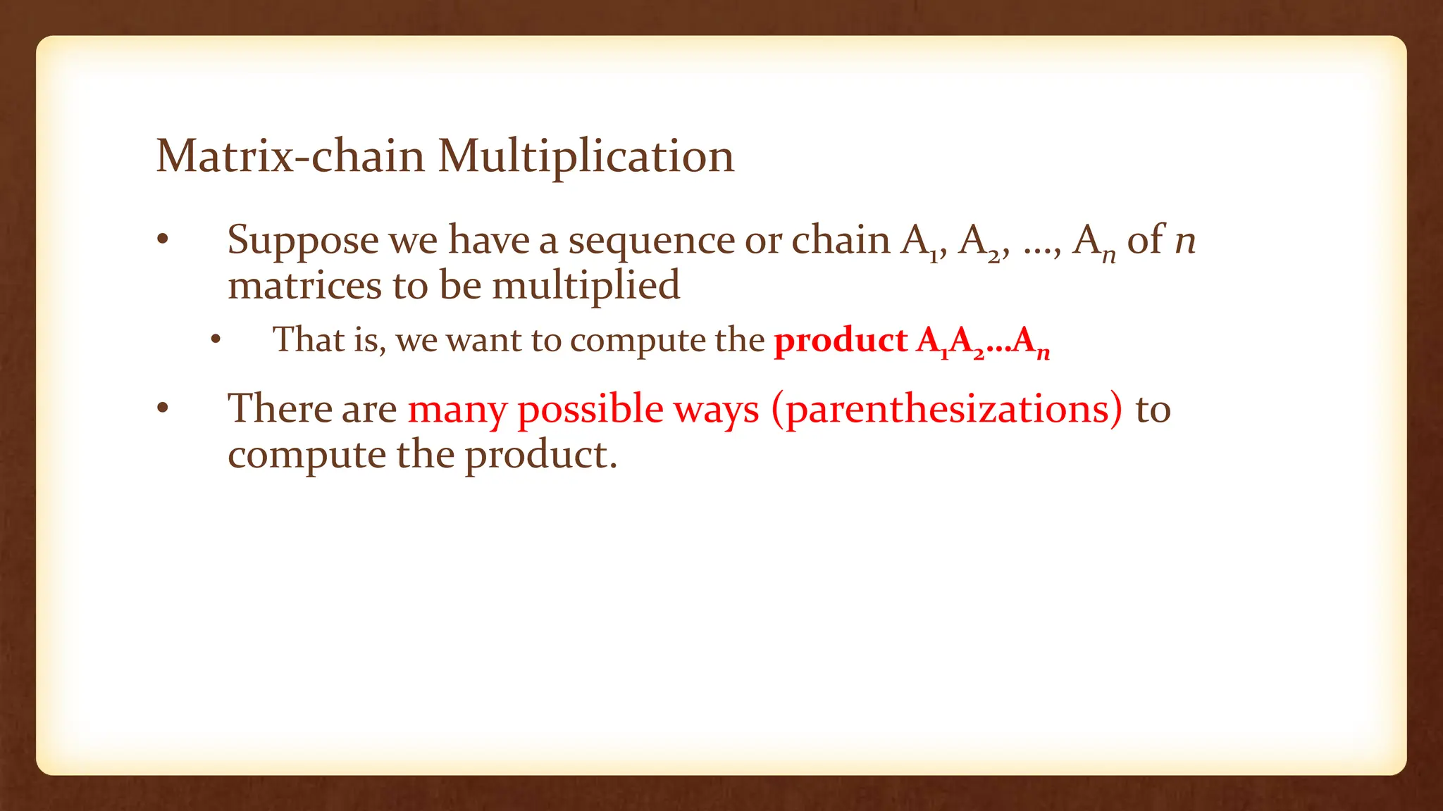
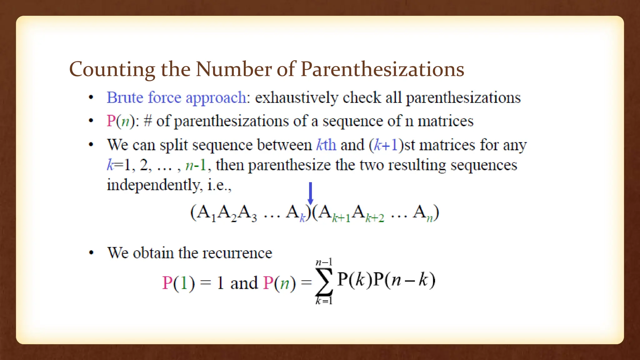
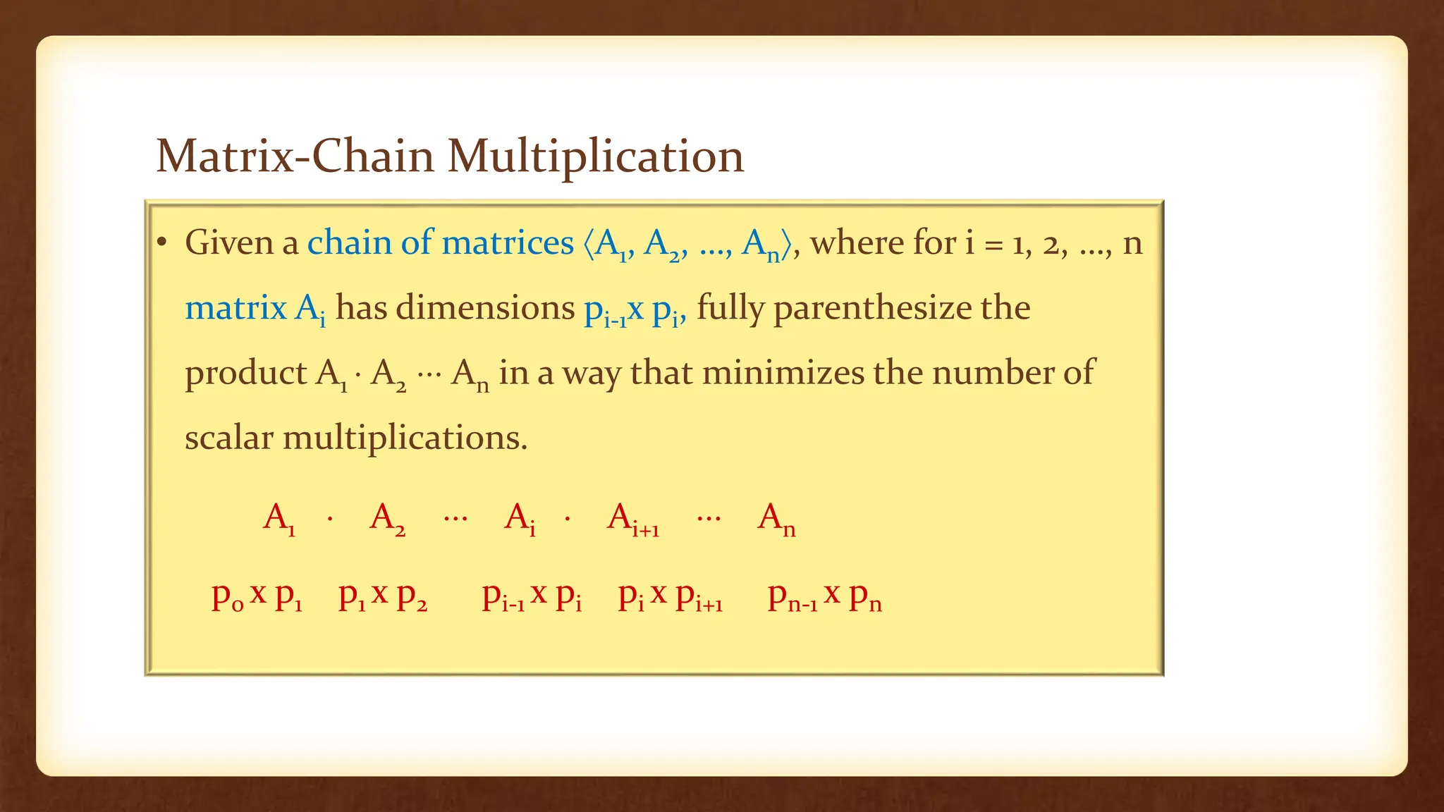
- The problem is to find the most efficient way to multiply a sequence of matrices by determining the optimal parenthesization that minimizes the number of scalar multiplications.
- A dynamic programming approach is used where the problem is broken down into optimal subproblems and a bottom-up method is employed to compute the solution.
- Recursive formulas are defined to calculate the minimum number of multiplications (m) needed to compute matrix chain products of increasing length. Additional data (s) tracks the optimal splitting points.
- The algorithm fills a table from bottom to top and left to right using the
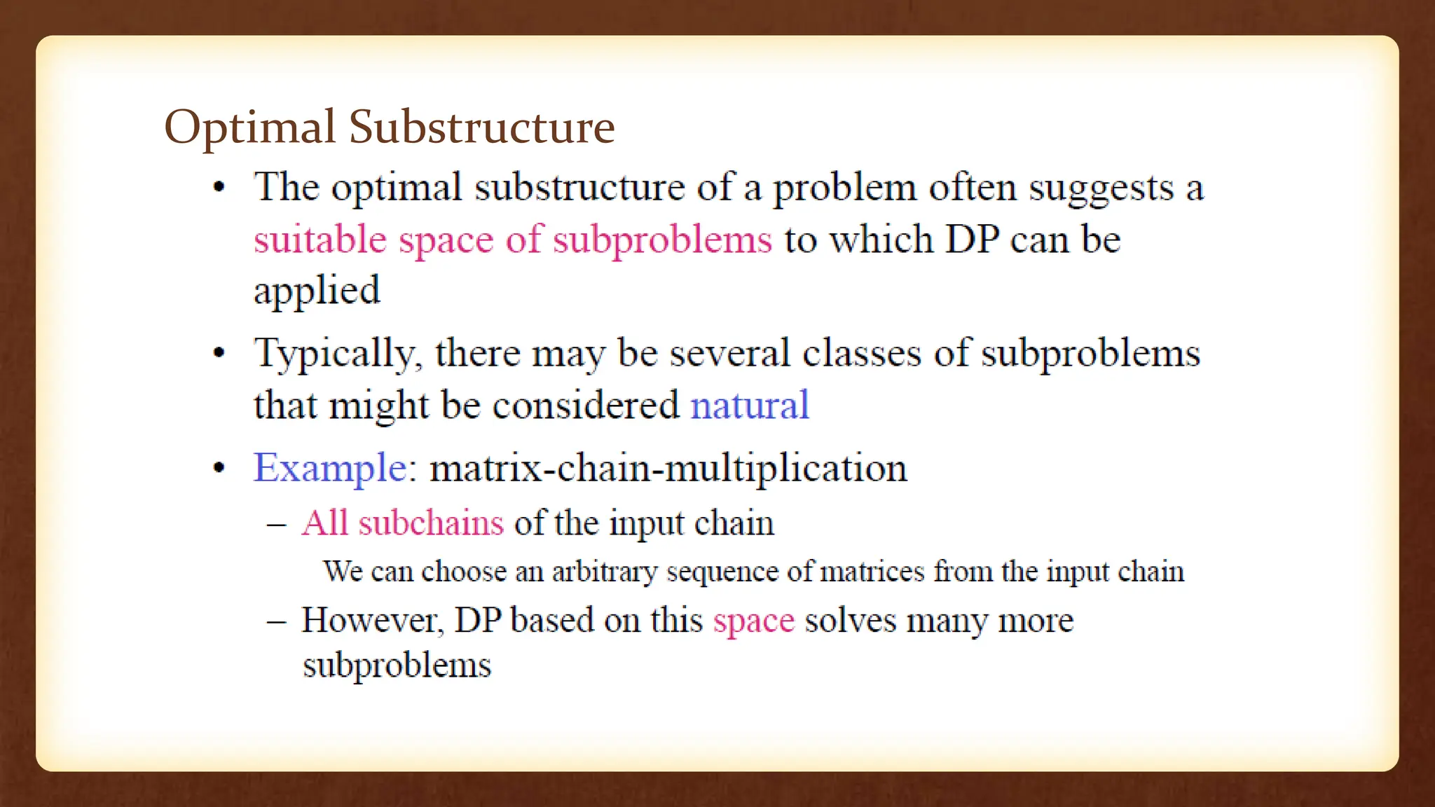
![Algorithm to Multiply 2 Matrices
Input: Matrices Ap×q and Bq×r (with dimensions p×q and q×r)
Result: Matrix Cp×r resulting from the product A·B
MATRIX-MULTIPLY(Ap×q , Bq×r)
1. for i ← 1 to p
2. for j ← 1 to r
3. C[i, j] ← 0
4. for k ← 1 to q
5. C[i, j] ← C[i, j] + A[i, k] · B[k, j]
6. return C
Scalar multiplication in line 5 dominates time to
compute C Number of scalar multiplications = pqr](https://image.slidesharecdn.com/matrixchainmultiplication-240316024602-5ead9b2f/75/Matrix-chain-multiplication-in-design-analysis-of-algorithm-4-2048.jpg)


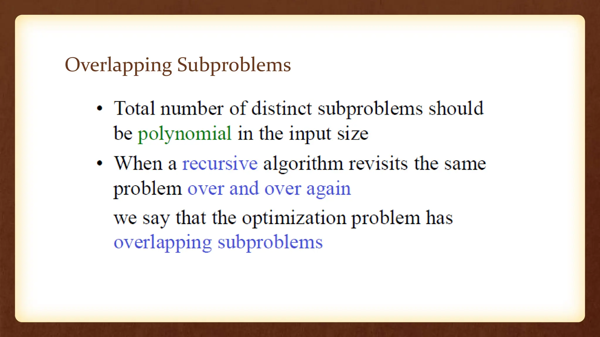
![2. A Recursive Solution
Step 2: Define the value of optimal solution recursively
• Subproblem:
Determine the minimum cost of parenthesizing
Ai…j = Ai Ai+1 Aj for 1 i j n
• Let m[i, j] = the minimum number of multiplications needed to compute Ai…j
• Full problem (A1..n): m[1, n]](https://image.slidesharecdn.com/matrixchainmultiplication-240316024602-5ead9b2f/75/Matrix-chain-multiplication-in-design-analysis-of-algorithm-18-2048.jpg)
![2. A Recursive Solution ….
Define m recursively:
• i = j: Ai…i = Ai m[i, i] = 0, for i = 1, 2, …, n , since the sub-chain contain just
one matrix; no multiplication at all.
• i < j: assume that the optimal parenthesization splits the product
Ai Ai+1 Aj between Ak and Ak+1, i k < j
Ai…j = Ai…k Ak+1…j
m[i, j] = m[i, k] + m[k+1, j] + pi-1pkpj
Ai…k Ak+1…j
Ai…kAk+1…j](https://image.slidesharecdn.com/matrixchainmultiplication-240316024602-5ead9b2f/75/Matrix-chain-multiplication-in-design-analysis-of-algorithm-19-2048.jpg)
![2. A Recursive Solution …..
• Consider the subproblem of parenthesizing
Ai…j = Ai Ai+1 Aj for 1 i j n
= Ai…k Ak+1…j for i k < j
• m[i, j] = the minimum number of multiplications needed to
compute the product Ai…j
m[i, j] = m[i, k] + m[k+1, j] + pi-1pkpj
min # of multiplications
to compute Ai…k
# of multiplications
to compute Ai…kAk…j
min # of multiplications
to compute Ak+1…j
m[i, k] m[k+1,j]
pi-1pkpj](https://image.slidesharecdn.com/matrixchainmultiplication-240316024602-5ead9b2f/75/Matrix-chain-multiplication-in-design-analysis-of-algorithm-20-2048.jpg)
![2. A Recursive Solution ….
m[i, j] = m[i, k] + m[k+1, j] + pi-1pkpj
• We do not know the value of k
• There are j – i possible values for k: k = i, i+1, …, j-1
• Minimizing the cost of parenthesizing the product Ai Ai+1 Aj
becomes:
0 if i = j
m[i, j] = min {m[i, k] + m[k+1, j] + pi-1pkpj} if i < j
ik<j](https://image.slidesharecdn.com/matrixchainmultiplication-240316024602-5ead9b2f/75/Matrix-chain-multiplication-in-design-analysis-of-algorithm-21-2048.jpg)
![Reconstructing the Optimal Solution
• Additional information to maintain:
• s[i, j] = a value of k at which we can split the product
Ai Ai+1 Aj in order to obtain an optimal parenthesization](https://image.slidesharecdn.com/matrixchainmultiplication-240316024602-5ead9b2f/75/Matrix-chain-multiplication-in-design-analysis-of-algorithm-22-2048.jpg)
![3. Computing the Optimal Costs
0 if i = j
m[i, j] = min {m[i, k] + m[k+1, j] + pi-1pkpj} if i < j
ik<j
• A recurrent algorithm may encounter each subproblem many
times in different branches of the recursion overlapping
subproblems
• Compute a solution using a tabular bottom-up approach](https://image.slidesharecdn.com/matrixchainmultiplication-240316024602-5ead9b2f/75/Matrix-chain-multiplication-in-design-analysis-of-algorithm-23-2048.jpg)
![3. Computing the Optimal Costs …
0 if i = j
m[i, j] = min {m[i, k] + m[k+1, j] + pi-1pkpj} if i < j
ik<j
• Length = 0: i = j, i = 1, 2, …, n
• Length = 1: j = i + 1, i = 1, 2, …, n-1
1
1
2 3 n
2
3
n
Compute rows from bottom to top
and from left to right
In a similar matrix s we keep the
optimal values of k
m[1, n] gives the optimal
solution to the problem
i
j](https://image.slidesharecdn.com/matrixchainmultiplication-240316024602-5ead9b2f/75/Matrix-chain-multiplication-in-design-analysis-of-algorithm-24-2048.jpg)
![Example: min {m[i, k] + m[k+1, j] + pi-1pkpj}
m[2, 2] + m[3, 5] + p1p2p5
m[2, 3] + m[4, 5] + p1p3p5
m[2, 4] + m[5, 5] + p1p4p5
1
1
2 3 6
2
3
6
i
j
4 5
4
5
m[2, 5] = min
• Values m[i, j] depend only
on values that have been
previously computed
k = 2
k = 3
k = 4](https://image.slidesharecdn.com/matrixchainmultiplication-240316024602-5ead9b2f/75/Matrix-chain-multiplication-in-design-analysis-of-algorithm-25-2048.jpg)
![Example
Compute A1 A2 A3
• A1: 10 x 100 (p0 x p1)
• A2: 100 x 5 (p1 x p2)
• A3: 5 x 50 (p2 x p3)
m[i, i] = 0 for i = 1, 2, 3
m[1, 2] = m[1, 1] + m[2, 2] + p0p1p2 (A1A2)
= 0 + 0 + 10 *100* 5 = 5,000
m[2, 3] = m[2, 2] + m[3, 3] + p1p2p3 (A2A3)
= 0 + 0 + 100 * 5 * 50 = 25,000
m[1, 3] = min m[1, 1] + m[2, 3] + p0p1p3 = 75,000 (A1(A2A3))
m[1, 2] + m[3, 3] + p0p2p3 = 7,500 ((A1A2)A3)
0
0
0
1
1
2
2
3
3
5000
1
25000
2
7500
2](https://image.slidesharecdn.com/matrixchainmultiplication-240316024602-5ead9b2f/75/Matrix-chain-multiplication-in-design-analysis-of-algorithm-26-2048.jpg)
![1. n length[p] – 1
2. for i 1 to n
3. do m[i, i] 0
4. for l 2 to n,
5. do for i 1 to n-l+1
6. do j i+l-1
7. m[i, j]
8. for k i to j-1
9. do q m[i, k] + m[k+1, j] + pi-1 . pk . pj
10. if q < m[i, j]
11. then m[i, j] = q
12. s[i, j] k
13. return m and s, “l is chain length”
Algorithm Chain-Matrix-Order(p)
m[1,4] m[2,4] m[3,4] m[4,4]
m[1,3] m[2,3] m[3,3]
m[1,2] m[2,2]
m[1,1]
1 2 3 4
4
3
2
1](https://image.slidesharecdn.com/matrixchainmultiplication-240316024602-5ead9b2f/75/Matrix-chain-multiplication-in-design-analysis-of-algorithm-27-2048.jpg)
![• Problem: Compute optimal multiplication order
for a series of matrices given below
20
50
.
50
5
.
5
100
.
100
10
4
3
2
1
A
A
A
A
m[1,4] m[2,4] m[3,4] m[4,4]
m[1,3] m[2,3] m[3,3]
m[1,2] m[2,2]
m[1,1]
P0 = 10
P1 = 100
P2 = 5
P3 = 50
P4 = 20
Example: Dynamic Programming
1 2 3 4
4
3
2
1](https://image.slidesharecdn.com/matrixchainmultiplication-240316024602-5ead9b2f/75/Matrix-chain-multiplication-in-design-analysis-of-algorithm-28-2048.jpg)
![Main Diagonal
• m[1, 1] = 0
• m[2, 2] = 0
• m[3, 3] = 0
• m[4, 4] = 0
)
.
.
]
,
1
[
]
,
[
(
]
,
[
4
,...,
1
,
0
]
,
[
1
min j
k
i
j
k
i
p
p
p
j
k
m
k
i
m
j
i
m
i
i
i
m
+
+
+
Main Diagonal
m[1,4] m[2,4] m[3,4] 0
m[1,3] m[2,3] 0
m[1,2] 0
0
1 2 3 4
4
3
2
1](https://image.slidesharecdn.com/matrixchainmultiplication-240316024602-5ead9b2f/75/Matrix-chain-multiplication-in-design-analysis-of-algorithm-29-2048.jpg)
![m[3, 4] = 0 + 0 + 5 . 50 . 20
= 5000
s[3, 4] = k = 3
)
.
.
]
,
1
[
]
,
[
(
]
,
[ 1
min j
k
i
j
k
i
p
p
p
j
k
m
k
i
m
j
i
m
+
+
+
)
.
.
]
4
,
1
[
]
,
3
[
(
]
4
,
3
[ 4
2
4
3
min p
p
p
k
m
k
m
m k
k
+
+
+
)
.
.
]
4
,
4
[
]
3
,
3
[
(
]
4
,
3
[ 4
3
2
min p
p
p
m
m
m +
+
Computing m[3,4], 4]
m[1,4] m[2,4] 3 5000 0
m[1,3] m[2,3] 0
m[1,2] 0
0
1 2 3 4
4
3
2
1](https://image.slidesharecdn.com/matrixchainmultiplication-240316024602-5ead9b2f/75/Matrix-chain-multiplication-in-design-analysis-of-algorithm-30-2048.jpg)
![m[2, 3] = 0 + 0 + 100 . 5 . 50
= 25000
s[2, 3] = k = 2
)
.
.
]
,
1
[
]
,
[
(
]
,
[ 1
min j
k
i
j
k
i
p
p
p
j
k
m
k
i
m
j
i
m
+
+
+
)
.
.
]
3
,
1
[
]
,
2
[
(
]
3
,
2
[ 3
1
3
2
min p
p
p
k
m
k
m
m k
k
+
+
+
)
3
.
.
]
3
,
3
[
]
2
,
2
[
(
]
3
,
2
[ 2
1
min p
p
p
m
m
m +
+
Computing m[2, 3]
m[1,4] m[2,4] 3 5000 0
m[1,3] 225000 0
m[1,2] 0
0
1 2 3 4
4
3
2
1](https://image.slidesharecdn.com/matrixchainmultiplication-240316024602-5ead9b2f/75/Matrix-chain-multiplication-in-design-analysis-of-algorithm-31-2048.jpg)
![m[1, 2] = 0 + 0 + 10 . 100 . 5
= 5000
s[1, 2] = k = 1
)
.
.
]
,
1
[
]
,
[
(
]
,
[ 1
min j
k
i
j
k
i
p
p
p
j
k
m
k
i
m
j
i
m
+
+
+
)
.
.
]
2
,
1
[
]
,
1
[
(
]
2
,
1
[ 2
0
2
1
min p
p
p
k
m
k
m
m k
k
+
+
+
)
.
.
]
2
,
2
[
]
1
,
1
[
(
]
2
,
1
[ 2
1
0
min p
p
p
m
m
m +
+
Computing m[1, 2]
m[1,4] m[2,4] 35000 0
m[1,3] 225000 0
1 5000 0
0
1 2 3 4
4
3
2
1](https://image.slidesharecdn.com/matrixchainmultiplication-240316024602-5ead9b2f/75/Matrix-chain-multiplication-in-design-analysis-of-algorithm-32-2048.jpg)
![m[2, 4] = min(0+5000+100.5.20, 25000+0+100.50.20)
= min(15000, 35000) = 15000
s[2, 4] = k = 2
)
.
.
]
,
1
[
]
,
[
(
]
,
[ 1
min j
k
i
j
k
i
p
p
p
j
k
m
k
i
m
j
i
m
+
+
+
)
.
.
]
4
,
1
[
]
,
2
[
(
]
4
,
2
[ 4
1
4
2
min p
p
p
k
m
k
m
m k
k
+
+
+
))
.
.
]
4
,
4
[
]
3
,
2
[
,
.
.
]
4
,
3
[
]
2
,
2
[
(
]
4
,
2
[
4
3
1
4
2
1
min
p
p
p
m
m
p
p
p
m
m
m
+
+
+
+
Computing m[2, 4]
m[1,4] 215000 3 5000 0
m[1,3] 225000 0
1 5000 0
0
1 2 3 4
4
3
2
1](https://image.slidesharecdn.com/matrixchainmultiplication-240316024602-5ead9b2f/75/Matrix-chain-multiplication-in-design-analysis-of-algorithm-33-2048.jpg)
![m[1, 3] = min(0+25000+10.100.50, 5000+0+10.5.50)
= min(75000, 2500) = 2500
s[1, 3] = k = 2
)
.
.
]
,
1
[
]
,
[
(
]
,
[ 1
min j
k
i
j
k
i
p
p
p
j
k
m
k
i
m
j
i
m
+
+
+
)
.
.
]
3
,
1
[
]
,
1
[
(
]
3
,
1
[ 3
0
3
1
min p
p
p
k
m
k
m
m k
k
+
+
+
))
.
.
]
3
,
3
[
]
2
,
1
[
,
.
.
]
3
,
2
[
]
1
,
1
[
(
]
3
,
1
[
3
2
0
3
1
0
min
p
p
p
m
m
p
p
p
m
m
m
+
+
+
+
Computing m[1, 3]
m[1,4] 215000 3 5000 0
2 2500 225000 0
1 5000 0
0
1 2 3 4
4
3
2
1](https://image.slidesharecdn.com/matrixchainmultiplication-240316024602-5ead9b2f/75/Matrix-chain-multiplication-in-design-analysis-of-algorithm-34-2048.jpg)
![m[1, 4] = min(0+15000+10.100.20, 5000+5000+
10.5.20, 2500+0+10.50.20)
= min(35000, 11000, 35000) = 11000
s[1, 4] = k = 2
)
.
.
]
,
1
[
]
,
[
(
]
,
[ 1
min j
k
i
j
k
i
p
p
p
j
k
m
k
i
m
j
i
m
+
+
+
)
.
.
]
4
,
1
[
]
,
1
[
(
]
4
,
1
[ 4
0
4
1
min p
p
p
k
m
k
m
m k
k
+
+
+
)
.
.
]
4
,
4
[
]
3
,
1
[
,
.
.
]
4
,
3
[
]
2
,
1
[
,
.
.
]
4
,
2
[
]
1
,
1
[
(
]
4
,
1
[
4
3
0
4
2
0
4
1
0
min
p
p
p
m
m
p
p
p
m
m
p
p
p
m
m
m
+
+
+
+
+
+
Computing m[1, 4]
211000 215000 3 5000 0
2 2500 225000 0
1 5000 0
0
4
3
2
1](https://image.slidesharecdn.com/matrixchainmultiplication-240316024602-5ead9b2f/75/Matrix-chain-multiplication-in-design-analysis-of-algorithm-35-2048.jpg)

![2 2 3 0
2 2 0
1 0
0
K,s Values Leading Minimum m[i, j]
1 2 3 4
4
3
2
1](https://image.slidesharecdn.com/matrixchainmultiplication-240316024602-5ead9b2f/75/Matrix-chain-multiplication-in-design-analysis-of-algorithm-37-2048.jpg)
![l = 2
10*20*25
=5000
35*15*5=
2625
l =3
m[3,5] = min
m[3,4]+m[5,5] + 15*10*20
=750 + 0 + 3000 = 3750
m[3,3]+m[4,5] + 15*5*20
=0 + 1000 + 1500 = 2500](https://image.slidesharecdn.com/matrixchainmultiplication-240316024602-5ead9b2f/75/Matrix-chain-multiplication-in-design-analysis-of-algorithm-38-2048.jpg)
![1. n length[p] – 1
2. for i 1 to n
3. do m[i, i] 0
4. for l 2 to n,
5. do for i 1 to n-l+1
6. do j i+l-1
7. m[i, j]
8. for k i to j-1
9. do q m[i, k] + m[k+1, j] + pi-1 . pk . pj
10. if q < m[i, j]
11. then m[i, j] = q
12. s[i, j] k
13. return m and s, “l is chain length”
Analysis Chain-Matrix-Order(p)
Takes O(n3) time
Requires O(n2) space](https://image.slidesharecdn.com/matrixchainmultiplication-240316024602-5ead9b2f/75/Matrix-chain-multiplication-in-design-analysis-of-algorithm-39-2048.jpg)
![11-40
• Our algorithm computes the minimum-
cost table m and the split table s
• The optimal solution can be constructed
from the split table s
• Each entry s[i, j ]=k shows where to split the
product Ai Ai+1 … Aj for the minimum cost.
4. Construct the Optimal Solution](https://image.slidesharecdn.com/matrixchainmultiplication-240316024602-5ead9b2f/75/Matrix-chain-multiplication-in-design-analysis-of-algorithm-40-2048.jpg)
![4. Construct the Optimal Solution …
• s[i, j] = value of k such that the optimal
parenthesization of Ai Ai+1 Aj splits the product between
Ak and Ak+1
3 3 3 5 5 -
3 3 3 4 -
3 3 3 -
1 2 -
1 -
-
1
1
2 3 6
2
3
6
i
j
4 5
4
5
• s[1, n] = 3 A1..6 = A1..3 A4..6
• s[1, 3] = 1 A1..3 = A1..1 A2..3
• s[4, 6] = 5 A4..6 = A4..5 A6..6
A1..n = A1..s[1, n] As[1, n]+1..n](https://image.slidesharecdn.com/matrixchainmultiplication-240316024602-5ead9b2f/75/Matrix-chain-multiplication-in-design-analysis-of-algorithm-41-2048.jpg)
![4. Construct the Optimal Solution …
3 3 3 5 5 -
3 3 3 4 -
3 3 3 -
1 2 -
1 -
-
1
1
2 3 6
2
3
6
i
j
4 5
4
5
PRINT-OPT-PARENS(s, i, j)
if i = j
then print “A”i
else print “(”
PRINT-OPT-PARENS(s, i, s[i, j])
PRINT-OPT-PARENS(s, s[i, j] + 1, j)
print “)”](https://image.slidesharecdn.com/matrixchainmultiplication-240316024602-5ead9b2f/75/Matrix-chain-multiplication-in-design-analysis-of-algorithm-42-2048.jpg)
![Example: A1 A6
3 3 3 5 5 -
3 3 3 4 -
3 3 3 -
1 2 -
1 -
-
1
1
2 3 6
2
3
6
i
j
4 5
4
5
PRINT-OPT-PARENS(s, i, j)
if i = j
then print “A”i
else print “(”
PRINT-OPT-PARENS(s, i, s[i, j])
PRINT-OPT-PARENS(s, s[i, j] + 1, j)
print “)”
P-O-P(s, 1, 6) s[1, 6] = 3
i = 1, j = 6 “(“ P-O-P (s, 1, 3) s[1, 3] = 1
i = 1, j = 3 “(“ P-O-P(s, 1, 1) “A1”
P-O-P(s, 2, 3) s[2, 3] = 2
i = 2, j = 3 “(“ P-O-P (s, 2, 2) “A2”
P-O-P (s, 3, 3) “A3”
“)”
“)”
( ( ( A4 A5 ) A6 ) )
A1 ( A2 A3 ) )
…
(
s[1..6, 1..6]](https://image.slidesharecdn.com/matrixchainmultiplication-240316024602-5ead9b2f/75/Matrix-chain-multiplication-in-design-analysis-of-algorithm-43-2048.jpg)