This document provides information about the Digital Signal Processing laboratory at Geethanjali College of Engineering and Technology, including:
- The cover page lists the college name and location, as well as the subject and laboratory manual details.
- It includes the JNTU syllabus and list of experiments for the DSP lab, vision and mission statements of the ECE department, and program educational objectives and outcomes.
- Guidelines for students and laboratory instructors are provided in the "Do's and Don'ts" section to ensure safety and effective learning in the lab.
- An introduction to digital signal processing concepts is given followed by a list of the experiments to be performed in the lab.
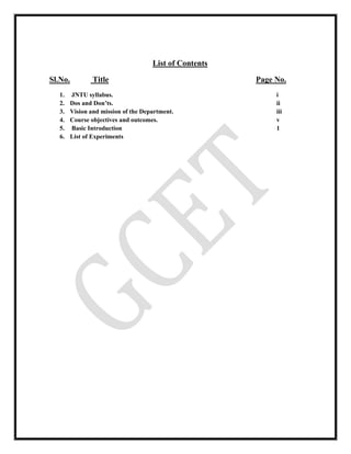


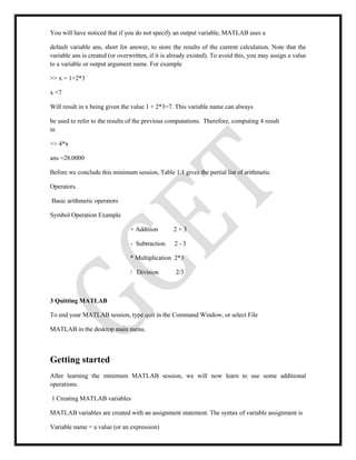
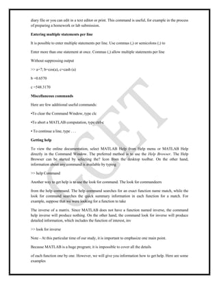


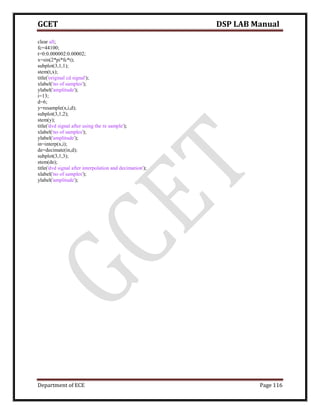
![1.GENERATION OF BASIC SIGNALS USING MATLAB
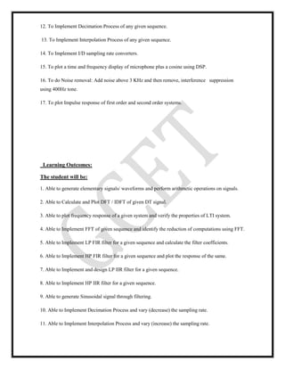
AIM : To generate basic signals like unit impulse, unit step, unit ramp signal and Exponential
signals.
Objective: To generate basic signals like unit impulse, unit step, unit ramp signal and Exponential
signals using MATlab.
Requirements : Computer with MATLAB software
(a). Program for the generation of UNIT impulse signal
clc; close all; clear all;
t=-2:1:2;
y=[zeros(1,2),ones(1,1),zeros(1,2)] figure(1)
subplot(2,2,1); stem(t,y);
title('unit impulse');
(b). Program for the generation of UNIT step signal
clc; close all; clear all;
n=input('enter the n value');
t=0:1:n-1;
y=ones(1,n);
figure(2)
subplot(2,2,2);
stem(t,y);
title('unit step');](https://image.slidesharecdn.com/dsplab-200213145717/85/Dsp-lab-22-320.jpg)

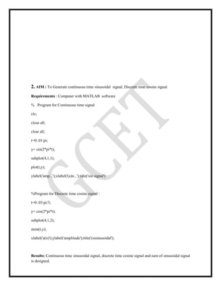
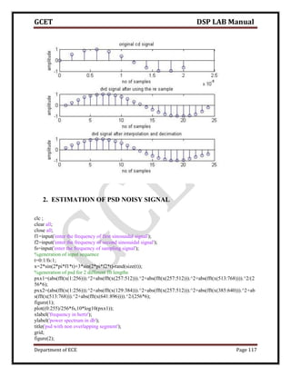
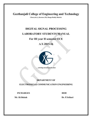
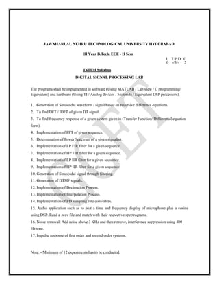
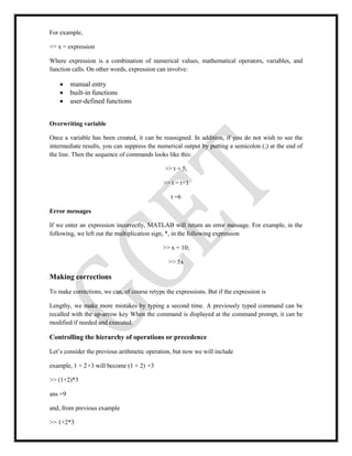
![FREQUENCY RESPONSE:
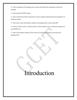
3. To find frequency response of a given system given in (Transfer Function/
Differential equation form).
AIM:- To write a MATLAB program to evaluate the Frequency response of the system .
Objective: To write a MATLAB program to evaluate the Frequency response of the system
.
EQUIPMENTS:
Operating System - Windows XP
Constructor - Simulator
Software - CCStudio 3 & MATLAB 7.5
THEORY:-
The Difference equation is given as
y[n]-0.25y[n-1]+0.45y[n-2]=1.55x[n]+1.95x[n-1]+ 2.15x[n]
The frequency response is a representation of the system's response to sinusoidal inputs at varying
frequencies. The output of a linear system to a sinusoidal input is a sinusoid of the same frequency
but with a different magnitude and phase. Any linear system can be completely described by how it
changes the amplitude and phase of cosine waves passing through it. This information is called the
system's frequency response. Since both the impulse response and the frequency response contain
complete information about the system, there must be a one-to-one correspondence between the
two. Given one, you can calculate the other. The relationship between the impulse response and the
frequency response is one of the foundations of signal processing: A system's frequency response is
the Fourier Transform of its impulse response Since h [ ] is the common symbol for the impulse
response, H [ ] is used for the frequency response.](https://image.slidesharecdn.com/dsplab-200213145717/85/Dsp-lab-26-320.jpg)
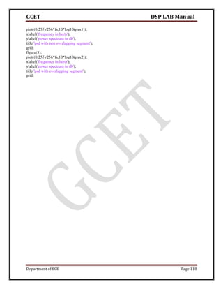
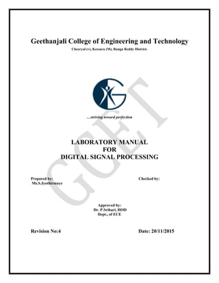
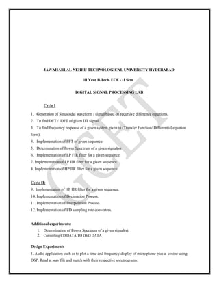
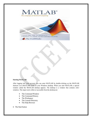
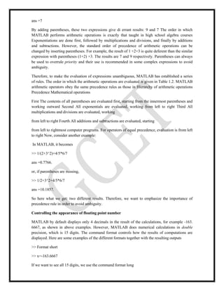
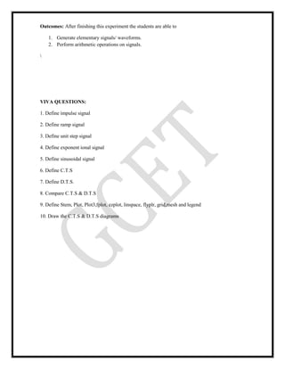
![PROGRAM:
clc;
clear all;
close all;
% Difference equation of a second order system
% y[n]-0.25y[n-1]+0.45y[n-2]=1.55x[n]+1.95x[n-1]+ 2.15x[n-2]
b=input('enter the coefficients of x(n),x(n-1)-----');
a=input('enter the coefficients of y(n),y(n-1)----');
N=input('enter the number of samples of frequency response ');
[h,t]=freqz(b,a,N);
subplot(2,1,1);
% figure(1);
plot(t,h);
subplot(2,1,2);
% figure(2);
stem(t,h);
title('plot of frequency response');
ylabel('amplitude');
xlabel('time index----->N');
disp(h);
grid on;
OUTPUT:
enter the coefficients of x(n),x(n-1)-----[1.55 1.95 2.15]
enter the coefficients of y(n),y(n-1)----[1 -.25 .45]
enter the number of samples of frequency response 1500](https://image.slidesharecdn.com/dsplab-200213145717/85/Dsp-lab-27-320.jpg)
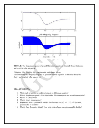

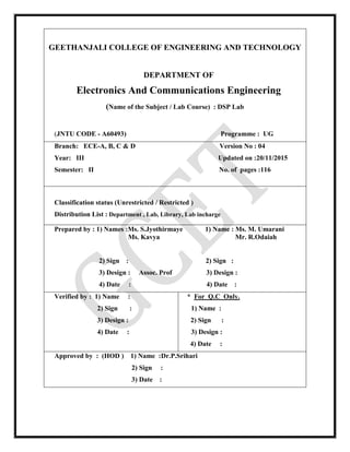
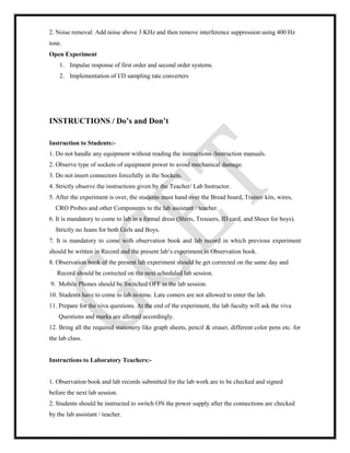
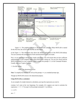
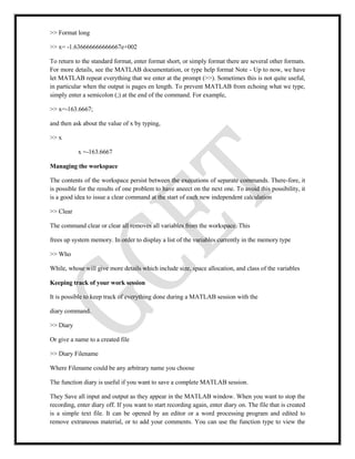
![The Difference equation is given as
y(n) = x(n)+0.5x(n-1)+0.85x(n-2)+y(n-1)+y(n-2)
THEORY:-
LTI Discrete time system is completely specified by its impulse response i.e. knowing the impulse
response we can compute the output of the system to any arbitrary input. Let h[n] denotes the
impulse response of the LTI discrete time systems. Since discrete time system is time invariant, its
response to [n-1] will be h[n-1] .Likewise the response to [n+2] , [n-4] and [n-6] will be h[n+2],
h[n-4] and h[n-6] .
From the above result arbitrary input sequence x[n] can be expressed as a weighted linear
combination of delayed and advanced unit sample in the form k=+
X[n] = x[k][n-k]
k=-
where weight x[k] on the right hand side denotes specifically the k th sample value of the sequence.
The response of the LTI discrete time system to the sequence
x[k] [n-k] will be x[k] h [n-k].
As a result, the response y[n] of the discrete time system to x[n] will be given by
k=+
y[n] = x[k] h [n-k] …………..(1)
k=-
Which can be alternately written as
k=+
y[n] = x[n-k] h [k]…………(2)
k=-
The above equation (1) and (2) is called the convolution sum of the sequences x[n]
and h[n] and represented compactly as y[n]=x[n] * h[n] Where the notation * denotes the
convolution sum.
Structure for Realization of Linear Time Invariant systems:
Let us consider the first order system Y(n)=-a 1y(n-1)+b0 x(n) +b1 x(n-1)
This realization uses separate delays(memory) for both the input and output samples and it is
called as Direct form one structure.
A close approximation reveals that the two delay elements contain the same input](https://image.slidesharecdn.com/dsplab-200213145717/85/Dsp-lab-30-320.jpg)
![w(n) and hence the same output w(n-1).consequently these two elements can be
merged into one delay. In contrast to the direct form I structure , this new realization
requires only one delay for auxiliary quantity w(n) ,and it is more efficient in terms
of memory requirements. It is called the direct form II structure and it is used
extensively.
PROGRAM:-
clc;
clear all;
close all;
% Difference equation of a second order system
% y(n) = x(n)+0.5x(n-1)+0.85x(n-2)+y(n-1)+y(n-2)
b=input('enter the coefficients of x(n),x(n-1)-----');
a=input('enter the coefficients of y(n),y(n-1)----');
N=input('enter the number of samples of imp response ');
[h,t]=impz(b,a,N);
subplot(2,1,1);
% figure(1);
plot(t,h);
title('plot of impulse response');
ylabel('amplitude');
xlabel('time index----->N');
subplot(2,1,2);
% figure(2);
stem(t,h);
title('plot of impulse response');
ylabel('amplitude');
xlabel('time index----->N');
disp(h);
grid on;
Output
enter the coefficients of x(n),x(n-1)-----[1 0.5 0.85] enter the coefficients of y(n),y(n-1)-----[1 -1 -1]
enter the number of samples of imp respons 4
1.0000](https://image.slidesharecdn.com/dsplab-200213145717/85/Dsp-lab-31-320.jpg)
![1.5000
3.3500
4.8500
GRAPH:-
CALCULATIONS:-
y(n) = x(n)+0.5x(n-1)+0.85x(n-2)+y(n-1)+y(n-2)
y(n) - y(n-1) - y(n-2) = x(n) + 0.5x(n-1) + 0.85x(n-2) Taking Z transform on both sides,
Y(Z) - Z-1 Y(Z)- Z-2 Y(Z) = X(Z) + 0.5 Z-1 X(Z) + 0.85 Z-2 X(Z) Y(Z)[1 - Z-1 - Z-2] = X(Z)[1 +
0.5 Z-1 + 0.85 Z-2 ]
But, H(Z) = Y(Z)/X(Z)](https://image.slidesharecdn.com/dsplab-200213145717/85/Dsp-lab-32-320.jpg)
![= [1 + 0.5 Z-1 + 0.85 Z-2 ]/ [1 - Z-1 - Z-2] By dividing we get
H(Z) = 1 + 1.5 Z-1 + 3.35 Z-2 + 4.85 Z-3
h(n) = [1 1.5 3.35 4.85]
RESULT: The impulse response of given Differential equation is obtained. Hence the theory and
practical value are proved
Outcome: The students are able to write the MATlab code to find the impulse response of given
Differential equation is obtained and the theory and practical value are proved
Discussion /Viva questions:-
1) Differentiate between linear and circular convolution.
2) Determine the unit step response of the linear time invariant system with impulse
response h(n)=a n
u(n) a<1&-a<1
3) Determine the range of values of the parameter a for which linear time
invariant system with impulse response h(n)=a n
u(n) is stable.
4) Consider the special case of a finite duration sequence given as X(n)={2 4 0 3}, resolve the sequence
x(n) into a sum of weighted sequences.
5) . Describe impulse response of a function?
6) . Where to use command filter or impz, and what is the difference between these two?
3. TO FIND DFT / IDFT OF GIVEN DT SIGNAL
AIM: To find the DFT / IDFT of given signal.
Objective: To wite the MATlab code to find the DFT / IDFT of given signal.](https://image.slidesharecdn.com/dsplab-200213145717/85/Dsp-lab-33-320.jpg)
![EQUIPMENTS:
Operating System - Windows XP
Constructor - Simulator
Software - CCStudio 3 & MATLAB 7.5
THEORY:
Discrete Time Fourier Transform:
The discrete-time Fourier transform (DTFT) X(ejω) of a sequence x[n] is defined
In general X(ejω) is a complex function of the real variable ω and can be written as
where Xre(ejω) and Xim(ejω) are, respectively, the real and imaginary parts of X(ejω), and are real
functions of ω. X(ejω) can alternately be expressed in the form
The quantity |X(ejω)| is called the magnitude function and the quantity θ(ω) is called the phase
function
In many applications, the Fourier transform is called the Fourier spectrum and, likewise, |X(ejω)|
and θ(ω) are referred to as the magnitude spectrum and phase spectrum, respectively.
The DTFT X(ejω) is a periodic continuous function in ω with a period 2π. The DTFT satisfies a
number of useful properties that are often uitilized in a number of applications.
MATLAB COMMANDS:
For complex Z, the magnitude R and phase angle theta are given by:
R = abs (Z)
Theta = angle (Z)
Y = fft(X) returns the discrete Fourier transform of vector X, computed with a fast Fourier
transform (FFT) algorithm.
Y = fft(X)
Y = fft(X,n) returns the n-point FFT.](https://image.slidesharecdn.com/dsplab-200213145717/85/Dsp-lab-34-320.jpg)
![Y = fft(X, n)
Compute the discrete Fourier transform of the following function analytically and Then plot the
magnitude and phase:
Its DTFT is given as:
MATLAB Code:
w = [0:500]*pi/500;
z = exp(-j*w);
x = 3*(1-0.9*z).^(-1);
a = abs(x);
b = angle(x)*180/pi;
subplot(2,1,1);
plot(w/pi,a);
subplot(2,1,2);
plot(w/pi,b);](https://image.slidesharecdn.com/dsplab-200213145717/85/Dsp-lab-35-320.jpg)
![Evaluate the DTFT of the given coefficients.
num=[2 1]
den=[1 –0.6]
Plot real and imaginary parts of Fourier spectrum.
Also plot the magnitude and phase spectrum.
MATLAB CODE:
% Evaluation of the DTFT
clc;
% Compute the frequency samples of the DTFT
w = -4*pi:8*pi/511:4*pi;
num = [2 1];
den = [1 -0.6];
h = freqz(num, den, w);
% Plot the DTFT
subplot(2,2,1)
plot(w/pi,real(h));
grid on;
title('Real part of H(e^{jomega})')
xlabel('omega /pi');
ylabel('Amplitude');
subplot(2,2,2)
plot(w/pi,imag(h));
grid on;
title('Imaginary part of H(e^{jomega})')
xlabel('omega /pi');
ylabel('Amplitude');
subplot(2,2,3)](https://image.slidesharecdn.com/dsplab-200213145717/85/Dsp-lab-36-320.jpg)
![plot(w/pi,abs(h));
grid on;
title('Magnitude Spectrum |H(e^{jomega})|')
xlabel('omega /pi');
ylabel('Amplitude');
subplot(2,2,4)
plot(w/pi,angle(h));
grid on;
title('Phase Spectrum arg[H(e^{jomega})]')
xlabel('omega /pi');
ylabel('Phase, radians');
PROGRAM:
Computation of N point DFT of a given sequence and to plot magnitude and phase
spectrum.](https://image.slidesharecdn.com/dsplab-200213145717/85/Dsp-lab-37-320.jpg)
![N = input('Enter the the value of N(Value of N in N-Point DFT)');
x = input('Enter the sequence for which DFT is to be calculated');
n=[0:1:N-1];
k=[0:1:N-1];
WN=exp(-1j*2*pi/N); % twiddle factor
nk=n'*k;
WNnk=WN.^nk;
Xk=x*WNnk;
MagX=abs(Xk) % Magnitude of calculated DFT
PhaseX=angle(Xk)*180/pi % Phase of the calculated DFT figure(1);
subplot(2,1,1);
plot(k,MagX);
subplot(2,1,2);
plot(k,PhaseX);
-------------*******--------------
OUTPUT
Enter the the value of N(Value of N in N-Point DFT)4 Enter the sequence for which DFT is to be
calculated [1 2 3 4]
MagX = 10.00002.8284 2.0000 2.8284
PhaseX = 0 135.0000 -180.0000 -135.0000
DFT of the given sequence is
10.0000-2.0000 + 2.0000i -2.0000 - 0.0000i -2.0000 -
2.0000i
Output:](https://image.slidesharecdn.com/dsplab-200213145717/85/Dsp-lab-38-320.jpg)

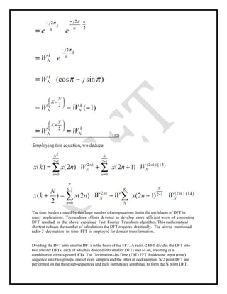
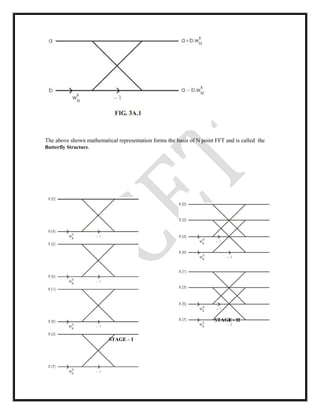
![STAGE - III
FIG. 3A.2 - 8 POINT DIT
Fast Fourier Transform:
The Fast Fourier Transform (FFT) is just a computationally fast way to calculate the DFT.
Question No 03: USING INBUILT FUNCTION
Determine the Fourier transform of the following sequence. Use the FFT (Fast Fourier
Transform) function.
x (n) = {4 6 2 1 7 4 8}
MATLAB Code: for defined sequence
n = 0:6;
x = [4 6 2 1 7 4 8];
a = fft(x);](https://image.slidesharecdn.com/dsplab-200213145717/85/Dsp-lab-44-320.jpg)
![mag = abs(a);
pha = angle(a);
subplot(2,1,1);
plot(mag);
grid on
title('Magnitude Response');
subplot(2,1,2);
plot(pha);
grid on
title('phase Response');
IMPLEMENTATION OF FFT OF GIVEN SEQUENCE IN MATLAB
N-POINT FFT WITHOUT USING INBUILT FUNCTION
PROGRAM:
clear all;
close all;
clc;
x=input('Enter the sequence x[n]= ');
N=input('Enter the value N point= ');
L=length(x);
x_n=[x,zeros(1,N-L)];
for i=1:N
for j=1:N
temp=-2*pi*(i-1)*(j-1)/N;
DFT_mat(i,j)=exp(complex(0,temp));
end
end
X_k=DFT_mat*x_n';
disp('N point DFT is X[k] = ');
disp(X_k);
mag=abs(X_k);
phase=angle(X_k)*180/pi;
subplot(2,1,1);
stem(mag);
xlabel('frequency index k');](https://image.slidesharecdn.com/dsplab-200213145717/85/Dsp-lab-45-320.jpg)
![ylabel('Magnitude of X[k]');
axis([0 N+1 -2 max(mag)+2]);
subplot(2,1,2);
stem(phase);
xlabel('frequency index k');
ylabel('Phase of X[k]');
axis([0 N+1 -180 180]);
PROGRAM: for user defined sequence
%fast fourier transform
clc;
clear all;
close all;
tic;
x=input('enter the sequence');
n=input('enter the length of fft'); %compute fft
disp('fourier transformed signal');
X=fft(x,n)
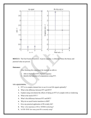
subplot(1,2,1);stem(x); title('i/p signal');
xlabel('n --->');
ylabel('x(n) -->');grid;
subplot(1,2,2);stem(X);
title('fft of i/p x(n) is:');
xlabel('Real axis --->');
ylabel('Imaginary axis -->');grid;
OUTPUT:-
enter the sequence[1 .25 .3 4]
enter the length of fft4
fourier transformed signal
X =
5.5500 0.7000 + 3.7500i -2.9500 0.7000 - 3.7500i
GRAPH FOR OUTPUT:-](https://image.slidesharecdn.com/dsplab-200213145717/85/Dsp-lab-46-320.jpg)

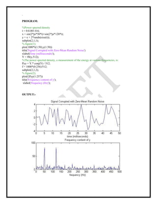
![5. Power Spectral Density
AIM: To verify Power Spectral Density
EQUIPMENTS:
Operating System - Windows XP
Constructor - Simulator
Software - CCStudio 3 & MATLAB 7.5
THEORY: The power spectral density(P.S.D) is a measurement of the energy at various
frequencies
In the previous section we saw how to unwrap the FFT and get back the sine and cosine
coefficients. Usually we only care how much information is contained at a particular frequency
and we don’t really care whether it is part of the sine or cosine series. Therefore, we are interested
in the absolute value of the FFT coefficients. The absolute value will provide you with the total
amount of information contained at a given frequency, the square of the absolute value is
considered the power of the signal. Remember that the absolute value of the Fourier coefficients
are the distance of the complex number from the origin. To get the power in the signal at
each frequency (commonly called the power spectrum) you can try the following commands.
>> N = 8; %% number of points
>> t = [0:N-1]’/N; %% define time
>> f = sin(2*pi*t); %%define function
>> p = abs(fft(f))/(N/2); %% absolute value of the fft
>> p = p(1:N/2).^2 %% take the positve frequency half, only
This set of commands will return something much easier to understand, you should get 1 at a
frequency of 1 and zeros everywhere else. Try substituting cos for sin in the above commands, you
should get the same result. Now try making >>f = sin(2*pi*t) + cos(2*pi*t). This change should
result in twice the power contained at a frequency of 1.
Thus far we have looked at data that is defined on the time interval of 1 second, therefore we could
interpret the location in the number list as the frequency. If the data is taken over an arbitrary time
interval we need to map the index into the Fourier series back to a frequency in Hertz. The
following m-file script will create something that might look like data that we would obtain from a
sensor. We will](https://image.slidesharecdn.com/dsplab-200213145717/85/Dsp-lab-49-320.jpg)
![1. FIR (finite impulse response) filter
2. IIR (infinite impulse response) filter
Description Of The Commands Used In FIR Filter Design
FIR1: FIR filters design using the window method.
B = FIR1(N,Wn) designs an N'th order low
pass FIR digital filter and returns the filter coefficients in length N+1 vector B. The cut-
off frequency Wn must be between 0 < Wn < 1.0, with 1.0 corresponding to half the
sample rate. The filter B is real and has linear phase. The normalized gain of the filter
at Wn is -6 dB.
B = FIR1(N,Wn,'high') designs an N'th order highpass filter.
You can also use B = FIR1(N,Wn,'low') to design a lowpass filter.
If Wn is a two-element vector, Wn = [W1 W2], FIR1 returns an order N bandpass filter with
passband W1 < W < W2.
B = FIR1(N,Wn,'stop') is a bandstop filter if Wn = [W1 W2]. You can also specify If Wn is a
multi-element vector, Wn = [W1 W2 W3 W4 W5 ... WN], FIR1 returns an order N multiband filter
with bands 0 < W < W1, W1 < W < W2, ..., WN < W < 1.
B = FIR1(N,Wn,'DC-1') makes the first band a passband.
B = FIR1(N,Wn,'DC-0') makes the first band a stopband.
By default FIR1 uses a Hamming window. Other available windows, including Boxcar, Hann,
Bartlett, Blackman, Kaiser and Chebwin can be specified with an optional trailing argument.
For example, B = FIR1(N,Wn,kaiser(N+1,4)) uses a Kaiser window with beta=4.
B = FIR1(N,Wn,'high', chebwin(N+1,R)) uses a Chebyshev window.
For filters with a gain other than zero at Fs/2, e.g., highpass and bandstop filters, N must
be even. Otherwise, N will be incremented by one. In this case the window length
should be specified as N+2.](https://image.slidesharecdn.com/dsplab-200213145717/85/Dsp-lab-52-320.jpg)
![By default, the filter is scaled so the center of the first pass band has magnitude exactly one after
windowing. Use a trailing 'noscale' argument to prevent this scaling, e.g.
B = FIR1(N,Wn,'noscale')
B = FIR1(N,Wn,'high','noscale')
B = FIR1(N,Wn,wind,'noscale').
You can also specify the scaling explicitly, e.g. FIR1(N,Wn,'scale'), etc.
FREQZ Digital Filter Frequency Response.
[H,W] = FREQZ(B,A,N) returns the N-point complex frequency response vector H and
the N-point frequency vector W in radians/sample of the filter: given numerator and
denominator coefficients in vectors B and A. The frequency response is evaluated at N
points equally spaced around the upper half of the unit circle. If N isn't specified, it
defaults to 512.
[H,W] = FREQZ(B,A,N,'whole') uses N points around the whole unit circle.
H = FREQZ(B,A,W) returns the frequency response at frequencies designated in vector W, in
radians/sample (normally between 0 and pi).
[H,F] = FREQZ(B,A,N,Fs) and [H,F] = FREQZ(B,A,N,'whole',Fs) return frequency vector F (in
Hz), where Fs is the sampling frequency (in Hz).
H = FREQZ(B,A,F,Fs) returns the complex frequency response at the frequencies designated in
vector F (in Hz), where Fs is the sampling frequency (in Hz).
[H,W,S] = FREQZ(...) or [H,F,S] = FREQZ(...) returns plotting information to be used with
FREQZPLOT. S is a structure whose fields can be altered to obtain different frequency response
plots. For more information see the help for FREQZPLOT.
FREQZ(B,A,...) with no output arguments plots the magnitude and unwrapped phase of the filter
in the current figure window.](https://image.slidesharecdn.com/dsplab-200213145717/85/Dsp-lab-53-320.jpg)
![DESIGNING A LOW PASS FILTER:
Suppose the target is to pass all frequencies below 1200 Hz
fs=8000; % sampling frequency
n=50; % order of the filter
w=1200/ (fs/2);
b=fir1(n,w,'low'); % Zeros of the filter
freqz(b,1,128,8000); % Magnitude and Phase Plot of the filter figure(2)
[h,w]=freqz(b,1,128,8000);
subplot(2,1,1);
plot(w,abs(h));% Normalized Magnitude Plot
title('Normalized Magnitude Plot');
grid
subplot(2,1,2);
figure(2)
zplane(b,1); % the plot in lab
title('zplane');
DESIGNING HIGH PASS FILTER:](https://image.slidesharecdn.com/dsplab-200213145717/85/Dsp-lab-54-320.jpg)
![Now the target is to pass all frequencies above 1200 Hz
fs=8000;
n=50;
w=1200/ (fs/2);
b=fir1(n,w,'high');
freqz(b,1,128,8000); % this function plots the phase(degree)and magnitude in db
subplot(2,1,2)
figure(2)
[h,w]=freqz(b,1,128,8000);
plot(w,abs(h)); % Normalized Magnitude Plot
title('Magnitude Plot ');
grid
figure(3)
zplane(b,1); % this function plots fiq in zplane
Designing High Pass Filter:
fs=8000;
n=50;
w=1200/ (fs/2);](https://image.slidesharecdn.com/dsplab-200213145717/85/Dsp-lab-55-320.jpg)
![b=fir1(n,w,'high');
freqz(b,1,128,8000);
figure(2)
[h,w]=freqz(b,1,128,8000);
plot(w,abs(h)); % Normalized Magnitude Plot
grid
figure(3)
zplane(b,1);
Designing Band Pass Filter:
fs=8000;
n=40;
b=fir1(n,[1200/4000 1800/4000],’bandpass’); freqz(b,1,128,8000)
figure(2)
[h,w]=freqz(b,1,128,8000);
plot(w,abs(h)); % Normalized Magnitude Plot
grid
figure(3)
zplane(b,1);
Designing Notch Filter
fs=8000;
n=40;
b=fir1(n,[1500/4000 1550/4000],'stop'); freqz(b,1,128,8000)
figure(2)
[h,w]=freqz(b,1,128,8000);
plot(w,abs(h)); % Normalized Magnitude Plot
grid
figure(3)](https://image.slidesharecdn.com/dsplab-200213145717/85/Dsp-lab-56-320.jpg)
![zplane(b,1);
Designing Multi Band Filter
n=50;
w=[0.2 0.4 0.6];
b=fir1(n,w);
freqz(b,1,128,8000) figure(2)
[h,w]=freqz(b,1,128,8000);
plot(w,abs(h)); % Normalized Magnitude Plot
grid
figure(3)
zplane(b,1);
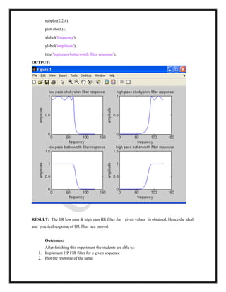
RESULT: The FIR low pass & high pass filter for given values is obtained. Hence the ideal
and practical response of FIR filter are proved.
Outcomes:
After finishing this experiment the students are able to:
1. Able to Implement LP FIR filter for a given sequence
2. Calculate the filter coefficients.
VIVA QUESTION:
1. What is filter?
2. What is FIR and IIR filter define, and distinguish between these two?
3. What is window method? How you will design an FIR filter using window method?
4. What are low-pass and band-pass filter and what is the difference between these two?
5. What is the matlab command for Hamming window? Explain.
6. What do you mean by built in function ‘abs’ and where it is used?
7. Explain how the FIR filter are stable?
8. Why is the impulse response "finite"?
9. What does "FIR" mean?
10. What are the advantages of FIR Filters (compared to IIR filters)?
11. What are the disadvantages of FIR Filters (compared to IIR filters)?
12. What terms are used in describing FIR filters?
13. What is the delay of a linear-phase FIR?](https://image.slidesharecdn.com/dsplab-200213145717/85/Dsp-lab-57-320.jpg)
![14. What is the Z transform of a FIR filter?
15. What is the frequency response formula for a FIR filter?
16. How Can I calculate the frequency response of a FIR using the Discrete Fourier Transform
(DFT)?
17. What is the DC gain of a FIR filter?
EXPERIMENT # 8 & 9
IMPLEMENTATION OF ANALOG IIR LOW PASS AND HIGH PASS FILTER FOR A
GIVEN SEQUENCE
AIM: To implementation of IIR low pass and high pass filter.
To verify Frequency response of analog IIR filter using MATLAB (LP/HP).
EQUIPMENTS:
Operating System - Windows XP
Constructor - Simulator
Software - CCStudio 3 & MATLAB 7.5
THEORY: Matlab contains various routines for design and analyzing digital filter IIR. Most of
these are part of the signal processing tool box. A selection of these filters is listed below.
Buttord ( for calculating the order of filter)
Butter ( creates an IIR filter)
Ellipord ( for calculating the order of filter) Ellip (creates an IIR filter)
Cheb1ord (for calculating the order of filter) Cheyb1 (creates an IIR filter)
Explanation Of The Commands For Filter Design: Buttord:
Butterworth filter order selection.
[N, Wn] = BUTTORD(Wp, Ws, Rp, Rs) returns the order N of the lowest order digital
Butterworth filter that loses no more than Rp dB in the pass band and has at least Rs dB of
attenuation in the stop band. Wp and Ws are the pass band and stop band edge frequencies,
normalized from 0 to 1 (where 1 corresponds to pi radians/sample).
For example
Low pass: Wp = .1, Ws = .2
High pass: Wp = .2, Ws = .1
Band pass: Wp = [.2 .7], Ws = [.1 .8]
Band stop: Wp = [.1 .8], Ws = [.2 .7]
BUTTORD also returns Wn, the Butterworth natural frequency (or, the "3 dB frequency") to
use with BUTTER to achieve the specifications.](https://image.slidesharecdn.com/dsplab-200213145717/85/Dsp-lab-58-320.jpg)
![[N, Wn] = BUTTORD(Wp, Ws, Rp, Rs, 's') does the computation for an analog filter, in which
case Wp and Ws are in radians/second. When Rp is chosen as 3 dB, the Wn in BUTTER is equal to
Wp in BUTTORD.
ELLIPORD: ELLIPTIC FILTER ORDER SELECTION.
[N, Wn] = ELLIPORD(Wp, Ws, Rp, Rs) returns the order N of the lowest order digital
elliptic filter that loses no more than Rp dB in the pass band and has at least Rs dB of
attenuation in the stop band Wp and Ws are the pass band and stop band edge
frequencies, normalized from 0 to 1 (where 1 corresponds to pi radians/sample).
For example
Low pass: Wp = .1, Ws = .2
High pass: Wp = .2, Ws = .1
Band pass: Wp = [.2 .7], Ws = [.1 .8]
Band stop: Wp = [.1 .8], Ws = [.2 .7]
ELLIPORD also returns Wn, the elliptic natural frequency to use with ELLIP to achieve the
specifications.
[N, Wn] = ELLIPORD(Wp, Ws, Rp, Rs, 's') does the computation for an analog filter, in which
case Wp and Ws are in radians/second. NOTE: If Rs is much greater than Rp, or Wp and Ws are
very close, the estimated order can be infinite due to limitations of numerical precision.
CHEB1ORD:CHEBYSHEV TYPE I FILTER ORDER SELECTION.
[N, Wn] = CHEB1ORD(Wp, Ws, Rp, Rs) returns the order N of the lowest order digital
Chebyshev Type I filter that loses no more than Rp dB in the pass band and has at least
Rs dB of attenuation in the stop band. Wp and Ws are the pass band and stop band edge
frequencies, normalized from 0 to 1 (where 1 corresponds to pi radians/sample).
For example,
Low pass: Wp = .1, Ws = .2
High pass: Wp = .2, Ws = .1
Band pass: Wp = [.2 .7], Ws = [.1 .8]
Band stop: Wp = [.1 .8], Ws = [.2 .7]
CHEB1ORD also returns Wn, the Chebyshev natural frequency to use with CHEBY1 to achieve
the specifications. [N, Wn] = CHEB1ORD(Wp, Ws, Rp, Rs, 's') does the computation for an
analog filter, in which case Wp and Ws are in radians/second.
BUTTER:BUTTERWORTH DIGITAL AND ANALOG FILTER DESIGN.
[B,A] = BUTTER(N,Wn) designs an Nth order lowpass digital Butterworth filter and
returns the filter coefficients in length N+1 vectors B (numerator) and A (denominator).
The coefficients are listed in descending powers of z. The cutoff frequency Wn must be
0.0 < Wn < 1.0, with 1.0 corresponding to half the sample rate.
If Wn is a two-element vector, Wn = [W1 W2], BUTTER returns an order 2N bandpass filter with
passband W1 < W < W2.](https://image.slidesharecdn.com/dsplab-200213145717/85/Dsp-lab-59-320.jpg)
![[B,A] = BUTTER(N,Wn,'high') designs a highpass filter.
[B,A] = BUTTER(N,Wn,'stop') is a bandstop filter if Wn = [W1 W2].
When used with three left-hand arguments, as in [Z,P,K] = BUTTER(...), the zeros and
poles are returned in length N column vectors Z and P, and the gain in scalar K. When
used with four left-hand arguments, as in [A,B,C,D] = BUTTER(...), state-space matrices
are returned.
BUTTER(N,Wn,'s'), BUTTER(N,Wn,'high','s') and BUTTER(N,Wn,'stop','s') design
analog Butterworth filters. In this case, Wn is in [rad/s] and it can be greater than 1.0.
ELLIP: ELLIPTIC OR CAUER DIGITAL AND ANALOG FILTER DESIGN.
[B,A] = ELLIP(N,Rp,Rs,Wn) designs an Nth order low pass digital elliptic filter with Rp
decibels of peak-to-peak ripple and a minimum stop band attenuation of Rs decibels.
ELLIP returns the filter coefficients in length N+1 vectors B (numerator) and A (denominator).The
cutoff frequency Wn must be 0.0 < Wn < 1.0, with 1.0 corresponding to half the sample rate. Use
Rp = 0.5 and Rs = 20 as starting points, if you are unsure about choosing them. If Wn is a two-
element vector, Wn = [W1 W2], ELLIP returns an order 2N band pass filter with pass band W1 <
W < W2. [B,A] = ELLIP(N,Rp,Rs,Wn,'high') designs a high pass filter.
[B,A] = ELLIP(N,Rp,Rs,Wn,'stop') is a band stop filter if Wn = [W1 W2].
When used with three left-hand arguments, as in [Z,P,K] = ELLIP(...), the zeros and
poles are returned in length N column vectors Z and P, and the gain in scalar K. When
used with four left-hand arguments, as in [A,B,C,D] = ELLIP(...), state-space matrices
are returned.
ELLIP(N,Rp,Rs,Wn,'s'), ELLIP(N,Rp,Rs,Wn,'high','s') and ELLIP(N,Rp,Rs,Wn,'stop','s')
design analog elliptic filters. In this case, Wn is in [rad/s] and it can be greater than 1.0.
CHEBY1: CHEBYSHEV TYPE I DIGITAL AND ANALOG FILTER DESIGN.
[B,A] = CHEBY1(N,R,Wn) designs an Nth order lowpass digital Chebyshev filter with R decibels
of peak-to-peak ripple in the passband. CHEBY1 returns the filter coefficients in length N+1
vectors B (numerator) and A (denominator). The cutoff frequency Wn must be 0.0 < Wn < 1.0,
with 1.0 corresponding to half the sample rate. Use R=0.5 as a starting point, if you are unsure
about choosing R.
If Wn is a two-element vector, Wn = [W1 W2], CHEBY1 returns an order 2N bandpass filter with
passband W1 < W < W2.
[B,A] = CHEBY1(N,R,Wn,'high') designs a highpass filter.
[B,A] = CHEBY1(N,R,Wn,'stop') is a bandstop filter if Wn = [W1 W2].
When used with three left-hand arguments, as in [Z,P,K] = CHEBY1(...), the zeros and poles are
returned in length N column vectors Z and P, and the gain in scalar K.
When used with four left-hand arguments, as in [A,B,C,D] = CHEBY1(...), state-space matrices are
returned.](https://image.slidesharecdn.com/dsplab-200213145717/85/Dsp-lab-60-320.jpg)
![CHEBY1(N,R,Wn,'s'), CHEBY1(N,R,Wn,'high','s') and CHEBY1(N,R,Wn,'stop','s')
design analog Chebyshev Type I filters.In this case, Wn is in [rad/s] and it can be greater
than 1.0.
ALGORITHM:
1. Get the pass band and stop band ripples.
2. Get the pass band and stop band edge frequencies.
3. Get the sampling frequency.
4. Calculate the order of the filter.
5. Find the window coefficients.
6. Draw the magnitude and phase responses.
PROCEDURE:
1) Enter the pass band ripple (rp) and stop band ripple (rs).
2) Enter the pass band frequency (fp) and stop band frequency (fs).
3) Get the sampling frequency (f).
4) Calculate the analog pass band edge frequencies, w1 and w2.
w1 = 2*fp/f w2 = 2*fs/f
5) Calculate the order and 3dB cutoff frequency of the analog filter. [Make use of the following
function] [n,wn]=buttord(w1,w2,rp,rs,’s’)
6) Design an nth order analog lowpass Butter worth filter using the following statement.
[b,a]=butter(n,wn,’s’)
7) Find the complex frequency response of the filter by using ‘freqs( )’ function
[h,om]=freqs(b,a,w) where, w = 0:.01:pi
This function returns complex frequency response vector ‘h’ and frequency vector ‘om’ in
radians/samples of the filter.
b(s) b(1)Snb-1+b(2)Snb-2+……………b(nb)
H(s)= ____ = _________________________________
a(s) a(1)Sna-1+a(2)Sna-2+…………..a(na)
Where a,b are the vectors containing the denominator and numerator coefficients.
8) Calculate the magnitude of the frequency response in decibels (dB) m=20*log10(abs(h))
9) Plot the magnitude response [magnitude in dB Vs normalized frequency (om/pi)]
10)Give relevant names to x and y axes and give an appropriate title for the plot.
11)Repeat the procedure for highpass, bandpass, bandstop filters.](https://image.slidesharecdn.com/dsplab-200213145717/85/Dsp-lab-61-320.jpg)
![12)Plot all the responses in a single figure window.[Make use of subplot( )].
9) Repeat the program for Chebyshev type-I and Chebyshev type-II filters.
PROGRAM CODE:
A. CHEBYSHEV LOW PASS FILTER
clc;
clear all;
wp=0.5; %%% chebyshev low pass filter;
ws=0.7;
rp=1;
rs=50;
[n,wn]=cheb1ord(wp,ws,rp,rs);
[b,a]=cheby1(n,rp,wn);
[h,w]=freqz(b,a,128);
subplot(2,2,1)
plot(abs(h));
xlabel('frequency');
ylabel('amplitude');
title('low pass chebyshev filter response');
B. BUTTER WORTH LOW PASS FILTER
wp=0.5; % butter worth low pass filter
ws=0.7;
rp=1;
rs=50;
[n,wn]=buttord(wp,ws,rp,rs);
n
[b,a]=butter(n,wn);
[h,w]=freqz(b,a,128);
subplot(2,2,3)](https://image.slidesharecdn.com/dsplab-200213145717/85/Dsp-lab-62-320.jpg)
![plot(abs(h));
xlabel('frequency');6
ylabel('amplitude');
title('low pass butterworth filter response');
9.A CHEBYSHEV HIGH PASS FILTER
wp=0.7; %%% chebyshev high pass filter
ws=0.5;
rp=1;
rs=30;
[n,wn]=cheb1ord(wp,ws,rp,rs);
[b,a]=cheby1(n,rp,wn, 'high');
[h,w]=freqz(b,a,128);
subplot(2,2,2)
plot(abs(h));
xlabel('frequency');
ylabel('amplitude');
title('high pass chebyshev filter response');
9.B BUTTER WORTH HIGH PASS FILTER
wp=0.7; %butter worth high pass filter
ws=0.5;
rp=1;
rs=30;
[n,wn]=buttord(wp,ws,rp,rs);
n
[b,a]=butter(n,wn,'high');
[h,w]=freqz(b,a,128);](https://image.slidesharecdn.com/dsplab-200213145717/85/Dsp-lab-63-320.jpg)
![VIVA QUESTION:
1. What do you mean by cut-off frequency?
2. Give the difference between analog and digital filter?
3. What is the difference between type 1 and type 2 filter structure?
4. what is the role of delay element in filter design?
5. Explain how the frequency is filter in filters?
6. Differences between Butterworth chebyshev filters?
7. Can IIR filters be Linear phase? how to make it linear Phase?
8. What is the special about minimum phase filter?
10. Generation of Sinusoidal signal through filtering
AIM : To generate the sinusoidal signal using filter.
EQUIPMENTS:
Operating System - Windows XP
Constructor - Simulator
Software - CCStudio 3 & MATLAB 7.5
PROGRAME:
clear all
close all
echo on
t0=.2; % signal duration
ts=0.001; % sampling interval
fc=250; % carrier frequency
fs=1/ts; % sampling frequency
t=[-t0/2:ts:t0/2]; % time vector
kf=100; % deviation constant
m=cos(2*pi*10*t); % the message signal
int_m(1)=0;
for i=1:length(t)-1 % integral of m
int_m(i+1)=int_m(i)+m(i)*ts;
echo off ;](https://image.slidesharecdn.com/dsplab-200213145717/85/Dsp-lab-65-320.jpg)
![end
echo on ;
u=cos(2*pi*fc*t+2*pi*kf*int_m); % modulated signal
%now lets filter the signal
[z,p] = butter(1,2*50/fs,'low');
filter_out = filter(50,[1 50],u); %this damn filter doesn't work!
subplot(2,1,1);
plot(t,u);
hold on;
plot(t,m,'r');
subplot(2,1,2);
plot(t,filter_out);
hold on;
plot(t,m,'r')
RESULT: The sinusoidal signal is generated from filter response for given values .
Outcome : At the end of the experiment the students are able to generate a sinusoidal signal is
generated from filter response for given values
VIVA QUESTION:
1. What is the special about minimum phase filter?
2. In signal processing, why we are much more interested in orthogonal transform?
3. How is the non-periodic nature of the input signal handled?
4. If a have two vectors how will i check the orthogonality of those vectors?](https://image.slidesharecdn.com/dsplab-200213145717/85/Dsp-lab-66-320.jpg)
![equation for decimation
To prevent aliasing, this system uses the lowpass filter H(z) before the M-fold decimator to
suppress the frequency contents above the frequency fs/(2M), which is the Nyquist frequency of the
output signal. This system produces the same results as an analog anti-aliasing filter with a cutoff
frequency of fs/(2M) followed by an analog-to-digital (A/D) converter with a sampling frequency
of fs/M. Because the system shown in the figure above is in the digital domain, H(z) is a digital anti-
aliasing filter.
PROGRAM:
Clc;
Close all;
Clear all;
N=input(‘ input length of the sine seq’);
M= input(‘ down sampling factor’);
fi= input(‘ input signal freq’); % generation of sine sequence
t=0:N-1;
L=input(‘ enter the factor value’);
m=0:N*L-1;
x=sin(2*pi*fi*m);
%generate the down sample signal
Y=x([1:m:length(x)]);
Y([1:L:length(x)])=x;
Subplot(2,1,1);
Stem(n,x(1:N));
Title(‘ input sequence’);
Xlable(‘time’);
Ylabel(‘amplitude’);
Subplot(2,1,2);
Stem(n, Y);
Title([‘ output sequence ‘,num2str(m)]);
Xlable(‘time’);
Ylabel(‘amplitude’);
RESULT: The decimator for a given sequence is observed for chosen factor M.
Hence the theory and practical is verified.
Outcome : At the end of the experiment the student is able to perform decimator for a given
sequence is observed for chosen factor M.](https://image.slidesharecdn.com/dsplab-200213145717/85/Dsp-lab-68-320.jpg)
![PROGRAME:
Clc;
Close all;
Clear all;
N=input(‘ input length of the sine seq’);
L= input(‘ up sampling factor’);
Fi= input(‘ input signal freq’);
t=0:N-1;
X=sin(2*pi*fi*t);
Y=zeros(1,L*length(x));
Y([1:L:length(x)])=x;
Subplot(2,1,1);
Stem(n,x);
Title(‘ input sequence’);
Xlable(‘time’);
Ylabel(‘amplitude’);
Subplot(2,1,2);
Stem(n, Y(1:length(x));
Title([‘ output sequence ‘,num2str(L)]);
Xlable(‘time’);
Ylabel(‘amplitude’);
RESULT: The interpolation of given sequence is observed for factor value L. Hence the theory
and practical are verified.
Outcome : At the end of the experiment the student is able to calculate the interpolation of given
sequence is observed for factor value L and prove the theory and practical same.
VIVA QUESTION:
1. How does polyphase filtering save computations in an interpolation filter?
2. Why do we need I&Q signals?
3. What is Interpolation and decimation filters and why we need it?
4. What are "upsampling" and "interpolation"?
5. Why interpolate,i needed for any signal/sequence?
6. What is the "interpolation factor"?
7. Which signals can be interpolated?
8. Can interpolate will happens in multiple stages? If yes give reason?
9. Give any example of a FIR interpolator?](https://image.slidesharecdn.com/dsplab-200213145717/85/Dsp-lab-70-320.jpg)

![1. Open code composer studio
2. Create a new project, give a meaningful name ,save into working folder, select target as
TMS320C6713,and select output file type is execution. out.
3. Click on file opennewsource file save it with .c extension in working folder and write .c-
code for desired task.
4. Add c-file to project as a source [path sourceadd files to projectadd c. file].
5. Add the linker command filehello .cmd.[path c.ccstudio-
v3.1tutorialdsk67/3HELLO1Hello.cmd]
6. Add the run time support library file rts6700.lib.[path c.ccstudio-v.3.1c600cg
toolslibrts6700.lib].
7. Compile the program [path projectcompile file]
10. Build the program [path projectbuild]
11.Connect the kit to the system through the USB cable
12. Then switch on the kit
13. And now check the DSK6713 diagnostics kit whether all the connections are
Made correctly or not](https://image.slidesharecdn.com/dsplab-200213145717/85/Dsp-lab-73-320.jpg)
![14. Then select [debugconnect] on the cc studio window
15. Load the program [fileload program]
16. Run the program [debugrun].](https://image.slidesharecdn.com/dsplab-200213145717/85/Dsp-lab-74-320.jpg)
![AIM: To verify Linear Convolution using Code Composer Studio.
PROGRAM CODE:
#include <stdio.h>
#include <math.h>
void butterfly(double *,double *,double *,double *,double *,double *);
int main( )
{
int i;
double x[8]={1,2,3,4,4,3,2,1};
//double x[8]={4,3,2,1,0,0,0,0};
double XR[8];
double XI[8]={0.0,0.0,0.0,0.0,0.0,0.0,0.0,0.0};
double WNR[4]={0.999969, 0.707092, 0.0, -0.707092};
double WNI[4]={0.0 , -0.707092,-0.999969,-0.707092};
double spectrum[8];
// store data in bit reversal order
XR[0]=x[0];
XR[1]=x[4];
XR[2]=x[2];
XR[3]=x[6];
XR[4]=x[1];
XR[5]=x[5];
XR[6]=x[3];
XR[7]=x[7];
// clrscr( );
// FIRST STAGE OF BUTTERFLY
butterfly(&XR[0],&XI[0],&XR[1],&XI[1],&WNR[0],&WNI[0]);
butterfly(&XR[2],&XI[2],&XR[3],&XI[3],&WNR[0],&WNI[0]);
butterfly(&XR[4],&XI[4],&XR[5],&XI[5],&WNR[0],&WNI[0]);
butterfly(&XR[6],&XI[6],&XR[7],&XI[7],&WNR[0],&WNI[0]);
// SECOND STAGE OF BUTTERFLY
butterfly(&XR[0],&XI[0],&XR[2],&XI[2],&WNR[0],&WNI[0]);
butterfly(&XR[1],&XI[1],&XR[3],&XI[3],&WNR[2],&WNI[2]);
butterfly(&XR[4],&XI[4],&XR[6],&XI[6],&WNR[0],&WNI[0]);
butterfly(&XR[5],&XI[5],&XR[7],&XI[7],&WNR[2],&WNI[2]);
// THIRD STAGE OF BUTTERFLY
butterfly(&XR[0],&XI[0],&XR[4],&XI[4],&WNR[0],&WNI[0]);
butterfly(&XR[1],&XI[1],&XR[5],&XI[5],&WNR[1],&WNI[1]);
butterfly(&XR[2],&XI[2],&XR[6],&XI[6],&WNR[2],&WNI[2]);
butterfly(&XR[3],&XI[3],&XR[7],&XI[7],&WNR[3],&WNI[3]);
for(i=0;i<8;i++)
{
XR[i]*=64.0;
XI[i]*=64.0;
}
for(i=0;i<8;i++)](https://image.slidesharecdn.com/dsplab-200213145717/85/Dsp-lab-76-320.jpg)
![{
printf("n FFT XR[%d] = %lf XI[%d]= %lf",i,XR[i],i,XI[i]);
}
return(0);
}
void butterfly(double *ar,double *ai,double *br,double *bi,double *wr,double *wi)
{
double tr,ti;
*ar/=4.0;
*ai/=4.0;
tr=*ar*2;
ti=*ai*2;
*br/=4.0;
*bi/=4.0;
*ar+=*br * *wr - *bi * *wi;
*ai+=*br * *wi + *bi * *wr;
*br= tr - *ar;
*bi= ti - *ai;
}
Expected Output:
XR[0]=19.9999070; XI[0]=0.000000;
XR[1]=-5.828134; XI[1]=-2.414237;
XR[2]=0.000813; XI[2]=-0.000093;
XR[3]=-0.171618; XI[3]=-0.414175;
XR[4]=0.000248; XI[4]=0.000000;
5&6 . FIR Filter (LP/HP) Using Windowing technique
Theory:](https://image.slidesharecdn.com/dsplab-200213145717/85/Dsp-lab-77-320.jpg)
![DESIGNING AN FIR FILTER :
Following are the steps to design linear phase FIR filters Using Windowing Method.
I. Clearly specify the filter specifications.
Eg: Order = 30;
Sampling Rate = 8000 samples/sec
Cut off Freq. = 400 Hz.
II. Compute the cut-off frequency Wc
Eg: Wc = 2*pie* fc / Fs
= 2*pie* 400/8000
= 0.1*pie
III. Compute the desired Impulse Response h d (n) using particular Window.
Eg: b_rect1=fir1(order, Wc , 'high',boxcar(31));
IV. Convolve input sequence with truncated Impulse Response x (n)*h (n).
AIM: To verify FIR filters using Code Composer Studio.
1. Rectangular window (High pass)
PROGRAM CODE:
#include "filtercfg.h"
#include "dsk6713.h"
#include "dsk6713_aic23.h"
#include "stdio.h"
//float filter_coeff[ ]={0.021665,0.022076,0.020224,0.015918,0.009129,
// -0.000000,-0.011158,-0.023877,-0.037558,-0.051511,
// -0.064994,-0.077266,-0.087636,-0.095507,-0.100422,
// 0.918834,-0.100422,-0.095507,-0.087636,-0.077266,
// -0.064994,-0.051511,-0.037558,-0.023877,-0.011158,
// -0.000000,0.009129,0.015918,0.020224,0.022076,
// 0.021665};
//FIR High pass Rectangular filter pass band range 400Hz- 3.5KHz
//float filter_coeff[ ]={0.000000,-0.013457,-0.023448,-0.025402,-0.017127,
// -0.000000,0.020933,0.038103,0.043547,0.031399,
// 0.000000,-0.047098,-0.101609,-0.152414,-0.188394,
// 0.805541,-0.188394,-0.152414,-0.101609,-0.047098,
// 0.000000,0.031399,0.043547,0.038103,0.020933,
// -0.000000,-0.017127,-0.025402,-0.023448,-0.013457,
// 0.000000};
/|/FIR High pass Rectangular filter pass band range 800Hz-3.5KHz
float filter_coeff[ ]={-0.020798,-0.013098,0.007416,0.024725,0.022944,
-0.000000,-0.028043,-0.037087,-0.013772,0.030562,](https://image.slidesharecdn.com/dsplab-200213145717/85/Dsp-lab-78-320.jpg)
![0.062393,0.045842,-0.032134,-0.148349,-0.252386,
0.686050,-0.252386,-0.148349,-0.032134,0.045842,
0.062393,0.030562,-0.013772,-0.037087,-0.028043,
-0.000000,0.022944,0.024725,0.007416,-0.013098,
-0.020798}:
//FIR High pass Rectangular filter pass band range 1200Hz-3.5KHz
//static short int in_buffer[100];
DSK6713_AIC23_Config
config={0x0017,0x0017,0x00d8,0x00d8,0x0011,0x0000,0x0000,0x0043,0x0081,0x0001};
void main( )
{
DSK6713_AIC23_CodecHandle hCodec;
Uint32 l_input, r_input,l_output, r_output;
DSK6713_init( );
hCodec = DSK6713_AIC23_openCodec(0, &config);
DSK6713_AIC23_setFreq(hCodec, 1);
while(1)
{
while(!DSK6713_AIC23_read(hCodec, &l_input));
while(!DSK6713_AIC23_read(hCodec, &r_input));
l_output=(Int16)FIR_FILTER(&filter_coeff ,l_input);
r_output=l_output;
while(!DSK6713_AIC23_write(hCodec, l_output));
while(!DSK6713_AIC23_write(hCodec, r_output));
}
DSK6713_AIC23_closeCodec(hCodec);
}
signed int FIR_FILTER(float * h, signed int x)
{
int i=0;
signed long output=0;
static short int in_buffer[100];
in_buffer[0] = x;
for(i=30;i>0;i--)
in_buffer[i] = in_buffer[i-1];
for(i=0;i<32;i++)
output = output + h[i] * in_buffer[i];
//output = x;
return(output);
}](https://image.slidesharecdn.com/dsplab-200213145717/85/Dsp-lab-79-320.jpg)
![Expected Output: observed the output in CRO with respect to input signal, it pass the signal at
range of frequency 1200-3.5KHz,and attenuate at other than pass band frequency
2. Rectangular window (Lowpass)
PROGRAM CODE:
#include "filtercfg.h"
#include "dsk6713.h"
#include "dsk6713_aic23.h"
#include "stdio.h"
//float filter_coeff[ ]={-0.008982,-0.017782,-0.025020,-0.029339,-0.029569,
// -0.024895,-0.014970,0.000000,0.019247,0.041491,
// 0.065053,0.088016,0.108421,0.124473,0.134729,
// 0.138255,0.134729,0.124473,0.108421,0.088016,
// 0.065053,0.041491,0.019247,0.000000,-0.014970,
// -0.024895,-0.029569,-0.029339,-0.025020,-0.017782,
// -0.008982};
//FIR Low pass Rectangular Filter pass band range 0-500Hz
//float filter_coeff[ ]={-0.015752,-0.023869,-0.018176,0.000000,0.021481,
// 0.033416,0.026254,-0.000000,-0.033755,-0.055693,
// -0.047257,0.000000,0.078762,0.167080,0.236286,
// 0.262448,0.236286,0.167080,0.078762,0.000000,
// -0.047257,-0.055693,-0.033755,-0.000000,0.026254,
// 0.033416,0.021481,0.000000,-0.018176,-0.023869,
// -0.015752};
//FIR Low pass Rectangular Filter pass band range 0-1000Hz
float filter_coeff[ ]={-0.020203,-0.016567,0.009656,0.027335,0.011411,
-0.023194,-0.033672,0.000000,0.043293,0.038657,
-0.025105,-0.082004,-0.041842,0.115971,0.303048,
0.386435,0.303048,0.115971,-0.041842,-0.082004,
-0.025105,0.038657,0.043293,0.000000,-0.033672,
-0.023194,0.011411,0.027335,0.009656,-0.016567,
-0.020203};
//FIR Low pass Rectangular Filter pass band range 0-1500Hz
//static short int in_buffer[100];
DSK6713_AIC23_Config
config={0x0017,0x0017,0x00d8,0x00d8,0x0011,0x0000,0x0000,0x0043,0x0081,0x0001};
void main( )
{
DSK6713_AIC23_CodecHandle hCodec;
Uint32 l_input, r_input,l_output, r_output;
DSK6713_init();
hCodec = DSK6713_AIC23_openCodec(0, &config);](https://image.slidesharecdn.com/dsplab-200213145717/85/Dsp-lab-80-320.jpg)
![DSK6713_AIC23_setFreq(hCodec, 1);
while(1)
{
while(!DSK6713_AIC23_read(hCodec, &l_input));
while(!DSK6713_AIC23_read(hCodec, &r_input));
l_output=(Int16)FIR_FILTER(&filter_coeff ,l_input);
r_output=l_output;
while(!DSK6713_AIC23_write(hCodec, l_output));
while(!DSK6713_AIC23_write(hCodec, r_output));
}
DSK6713_AIC23_closeCodec(hCodec);
}
signed int FIR_FILTER(float * h, signed int x)
{
int i=0;
signed long output=0;
static short int in_buffer[100];
in_buffer[0] = x;
for(i=30;i>0;i--)
in_buffer[i] = in_buffer[i-1];
for(i=0;i<32;i++)
output = output + h[i] * in_buffer[i];
//output = x;
return(output);
}
Expected Output: observed the output in CRO for low pass filter with respect to input signal, it
pass the signal at range of pass band frequency 0-1500KHz,and attenuate at other than pass band
frequency
3. Triangular window (Highpass)
PROGRAM CODE:
#include "filtercfg.h"
#include "dsk6713.h"
#include "dsk6713_aic23.h"
#include "stdio.h"](https://image.slidesharecdn.com/dsplab-200213145717/85/Dsp-lab-81-320.jpg)
![//float filter_coeff[]={0.000000,0.001445,0.002648,0.003127,0.002391,
// -0.000000,-0.004383,-0.010943,-0.019672,-0.030353,
// -0.042554,-0.055647,-0.068853,-0.081290,-0.092048,
// 0.902380,-0.092048,-0.081290,-0.068853,-0.055647,
// -0.042554,-0.030353,-0.019672,-0.010943,-0.004383,
// -0.000000,0.002391,0.003127,0.002648,0.001445,
// 0.000000};
//FIR High pass Triangular filter pass band range 400Hz-3.5KHz
//float filter_coeff[]={0.000000,-0.000897,-0.003126,-0.005080,-0.004567,
// -0.000000,0.008373,0.017782,0.023225,0.018839,
// 0.000000,-0.034539,-0.081287,-0.132092,-0.175834,
// 0.805541,-0.175834,-0.132092,-0.081287,-0.034539,
// 0.000000,0.018839,0.023225,0.017782,0.008373,
// -0.000000,-0.004567,-0.005080,-0.003126,-0.000897,
// 0.000000};
//FIR High pass Triangular filter pass band range 800Hz-3.5KHz
float filter_coeff[]={0.000000,-0.000901,0.001021,0.005105,0.006317,
-0.000000,-0.011581,-0.017868,-0.007583,0.018931,
0.042944,0.034707,-0.026541,-0.132736,-0.243196,
0.708287,-0.243196,-0.132736,-0.026541,0.034707,
0.042944,0.018931,-0.007583,-0.017868,-0.011581,
-0.000000,0.006317,0.005105,0.001021,-0.000901,
0.000000};
//FIR High pass Triangular filter pass band range 1200Hz-3.5KHz
//static short int in_buffer[100];
DSK6713_AIC23_Config
config={0x0017,0x0017,0x00d8,0x00d8,0x0011,0x0000,0x0000,0x0043,0x0081,0x0001};
void main( )
{
DSK6713_AIC23_CodecHandle hCodec;
Uint32 l_input, r_input,l_output, r_output;
DSK6713_init();
hCodec = DSK6713_AIC23_openCodec(0, &config);
DSK6713_AIC23_setFreq(hCodec, 1);
while(1)
{
while(!DSK6713_AIC23_read(hCodec, &l_input));
while(!DSK6713_AIC23_read(hCodec, &r_input));
l_output=(Int16)FIR_FILTER(&filter_coeff ,l_input);
r_output=l_output;
while(!DSK6713_AIC23_write(hCodec, l_output));](https://image.slidesharecdn.com/dsplab-200213145717/85/Dsp-lab-82-320.jpg)
![while(!DSK6713_AIC23_write(hCodec, r_output));
}
DSK6713_AIC23_closeCodec(hCodec);
}
signed int FIR_FILTER(float * h, signed int x)
{
int i=0;
signed long output=0;
static short int in_buffer[100];
in_buffer[0] = x;
for(i=30;i>0;i--)
in_buffer[i] = in_buffer[i-1];
for(i=0;i<32;i++)
output = output + h[i] * in_buffer[i];
//output = x;
return(output);
}
Expected Output: Observed the output in CRO with respect to input signal, it pass the signal at
range of pass band frequency 400-3.5KHz,and attenuate at other than pass band frequency
4. Triangular window (Lowpass)
PROGRAM CODE:
#include "filtercfg.h"
#include "dsk6713.h"
#include "dsk6713_aic23.h"
#include "stdio.h"
//float filter_coeff[ ]={0.000000,-0.001185,-0.003336,-0.005868,-0.007885,
// -0.008298,-0.005988,0.000000,0.010265,0.024895,
// 0.043368,0.064545,0.086737,0.107877,0.125747,
// 0.138255,0.125747,0.107877,0.086737,0.064545,
// 0.043368,0.024895,0.010265,0.000000,-0.005988,
// -0.008298,-0.007885,-0.005868,-0.003336,-0.001185,
// 0.000000};
//FIR Low pass Triangular Filter pass band range 0-500Hz
//float filter_coeff[ ]={0.000000,-0.001591,-0.002423,0.000000,0.005728,
// 0.011139,0.010502,-0.000000,-0.018003,-0.033416,
// -0.031505,0.000000,0.063010,0.144802,0.220534,
// 0.262448,0.220534,0.144802,0.063010,0.000000,
// -0.031505,-0.033416,-0.018003,-0.000000,0.010502,
// 0.011139,0.005728,0.000000,-0.002423,-0.001591,
// 0.000000};
//FIR Low pass Triangular Filter pass band range 0-1000Hz](https://image.slidesharecdn.com/dsplab-200213145717/85/Dsp-lab-83-320.jpg)
![float filter_coeff[ ]={0.000000,-0.001104,0.001287,0.005467,0.003043,
-0.007731,-0.013469,0.000000,0.023089,0.023194,
-0.016737,-0.060136,-0.033474,0.100508,0.282844,
0.386435,0.282844,0.100508,-0.033474,-0.060136,
-0.016737,0.023194,0.023089,0.000000,-0.013469,
-0.007731,0.003043,0.005467,0.001287,-0.001104,
0.000000};
//FIR Low pass Triangular Filter pass band range 0-1500Hz
//static short int in_buffer[100];
DSK6713_AIC23_Config
config={0x0017,0x0017,0x00d8,0x00d8,0x0011,0x0000,0x0000,0x0043,0x0081,0x0001};
void main( )
{
DSK6713_AIC23_CodecHandle hCodec;
Uint32 l_input, r_input,l_output, r_output;
DSK6713_init();
hCodec = DSK6713_AIC23_openCodec(0, &config);
DSK6713_AIC23_setFreq(hCodec, 1);
while(1)
{
while(!DSK6713_AIC23_read(hCodec, &l_input));
while(!DSK6713_AIC23_read(hCodec, &r_input));
l_output=(Int16)FIR_FILTER(&filter_coeff ,l_input);
r_output=l_output;
while(!DSK6713_AIC23_write(hCodec, l_output));
while(!DSK6713_AIC23_write(hCodec, r_output));
}
DSK6713_AIC23_closeCodec(hCodec);
}
signed int FIR_FILTER(float * h, signed int x)
{
int i=0;
signed long output=0;
static short int in_buffer[100];
in_buffer[0] = x;
for(i=30;i>0;i--)
in_buffer[i] = in_buffer[i-1];
for(i=0;i<32;i++)
output = output + h[i] * in_buffer[i];](https://image.slidesharecdn.com/dsplab-200213145717/85/Dsp-lab-84-320.jpg)
![//output = x;
return(output);
}
Expected Output: Observed the output in CRO with respect to input signal, it pass the signal at
range of pass band frequency 0-1500KHz,and attenuate at other than pass band frequency
5. Kaiser window (High pass)
PROGRAM CODE:
#include "filtercfg.h"
#include "dsk6713.h"
#include "dsk6713_aic23.h"
#include "stdio.h"
//float filter_coeff[ ]={0.000050,0.000223,0.000520,0.000831,0.000845,
// -0.000000,-0.002478,-0.007437,-0.015556,-0.027071,
// -0.041538,-0.057742,-0.073805,-0.087505,-0.096739,
// 0.899998,-0.096739,-0.087505,-0.073805,-0.057742,
// -0.041538,-0.027071,-0.015556,-0.007437,-0.002478,
// -0.000000,0.000845,0.000831,0.000520,0.000223,
// 0.000050};
//FIR High pass Kaiser filter pass band range 400Hz-3.5KHz
//float filter_coeff[ ]={0.000000,-0.000138,-0.000611,-0.001345,-0.001607,
// -0.000000,0.004714,0.012033,0.018287,0.016731,
// 0.000000,-0.035687,-0.086763,-0.141588,-0.184011,
// 0.800005,-0.184011,-0.141588,-0.086763,-0.035687,](https://image.slidesharecdn.com/dsplab-200213145717/85/Dsp-lab-85-320.jpg)
![// 0.000000,0.016731,0.018287,0.012033,0.004714,
// -0.000000,-0.001607,-0.001345,-0.000611,-0.000138,
// 0.000000};
//FIR High pass Kaiser filter pass band range 800Hz-3.5KHz
float filter_coeff[ ]={-0.000050,-0.000138,0.000198,0.001345,0.002212,-0.000000,
-0.006489,-0.012033,-0.005942,0.016731,0.041539,0.035687,
-0.028191,-0.141589,-0.253270,0.700008,-0.253270,-0.141589,
-0.028191,0.035687,0.041539,0.016731,-0.005942,-0.012033,
-0.006489,-0.000000,0.002212,0.001345,0.000198,-0.000138,
-0.000050};
//FIR High pass Kaiser filter pass band range 1200Hz-3.5KHz
//static short int in_buffer[100];
DSK6713_AIC23_Config
config={0x0017,0x0017,0x00d8,0x00d8,0x0011,0x0000,0x0000,0x0043,0x0081,0x0001};
void main( )
{
DSK6713_AIC23_CodecHandle hCodec;
Uint32 l_input, r_input,l_output, r_output;
DSK6713_init();
hCodec = DSK6713_AIC23_openCodec(0, &config);
DSK6713_AIC23_setFreq(hCodec, 1);
while(1)
{
while(!DSK6713_AIC23_read(hCodec, &l_input));
while(!DSK6713_AIC23_read(hCodec, &r_input));
l_output=(Int16)FIR_FILTER(&filter_coeff ,l_input);
r_output=l_output;
while(!DSK6713_AIC23_write(hCodec, l_output));
while(!DSK6713_AIC23_write(hCodec, r_output));
}
DSK6713_AIC23_closeCodec(hCodec);
}
signed int FIR_FILTER(float * h, signed int x)
{
int i=0;
signed long output=0;
static short int in_buffer[100];
in_buffer[0] = x;
for(i=30;i>0;i--)](https://image.slidesharecdn.com/dsplab-200213145717/85/Dsp-lab-86-320.jpg)
![in_buffer[i] = in_buffer[i-1];
for(i=0;i<32;i++)
output = output + h[i] * in_buffer[i];
//output = x;
return(output);
}
Expected Output: Observed the output in CRO with respect to input signal, it pass the signal at
range of pass band frequency 1200-3.5KHz,and attenuate at other than pass band frequency
6. Kaiser window (Low pass)
PROGRAM CODE:
#include "filtercfg.h"
#include "dsk6713.h"
#include "dsk6713_aic23.h"
#include "stdio.h"
//float filter_coeff[]={-0.000019,-0.000170,-0.000609,-0.001451,-0.002593,
// -0.003511,-0.003150,0.000000,0.007551,0.020655,
// 0.039383,0.062306,0.086494,0.108031,0.122944,
// 0.128279,0.122944,0.108031,0.086494,0.062306,
// 0.039383,0.020655,0.007551,0.000000,-0.003150,
// -0.003511,-0.002593,-0.001451,-0.000609,-0.000710,
// -0.000019};
// kaiser low pass fir filter pass band range 0-500Hz
//float filter_coeff[]={-0.000035,-0.000234,-0.000454,0.000000,0.001933,
// 0.004838,0.005671,-0.000000,-0.013596,-0.028462,
// -0.029370,0.000000,0.064504,0.148863,0.221349,
// 0.249983,0.221349,0.148863,0.064504,0.000000,
// -0.029370,-0.028462,-0.013596,-0.000000,0.005671,
// 0.004838,0.001933,0.000000,-0.000454,-0.000234,
// -0.000035};
// kaiser low pass fir filter pass band range 0-1000Hz](https://image.slidesharecdn.com/dsplab-200213145717/85/Dsp-lab-87-320.jpg)
![float filter_coeff[]={-0.000046,-0.000166,0.000246,0.001414,0.001046,
-0.003421,-0.007410,0.000000,0.017764,0.020126,
-0.015895,-0.060710,-0.034909,0.105263,0.289209,
0.374978,0.289209,0.105263,-0.034909,-0.060710,
-0.015895,0.020126,0.017764,0.000000,-0.007410,
-0.003421,0.001046,0.001414,0.000246,-0.000166,
-0.000046};
//Kaiser low pass fir filter pass band range 0-1500Hz
//static short int in_buffer[100];
DSK6713_AIC23_Config
config={0x0017,0x0017,0x00d8,0x00d8,0x0011,0x0000,0x0000,0x0043,0x0081,0x0001};
void main( )
{
DSK6713_AIC23_CodecHandle hCodec;
Uint32 l_input, r_input,l_output, r_output;
DSK6713_init();
hCodec = DSK6713_AIC23_openCodec(0, &config);
DSK6713_AIC23_setFreq(hCodec, 1);
while(1)
{
while(!DSK6713_AIC23_read(hCodec, &l_input));
while(!DSK6713_AIC23_read(hCodec, &r_input));
l_output=(Int16)FIR_FILTER(&filter_coeff ,l_input);
r_output=l_output;
while(!DSK6713_AIC23_write(hCodec, l_output));
while(!DSK6713_AIC23_write(hCodec, r_output));
}
DSK6713_AIC23_closeCodec(hCodec);
}
signed int FIR_FILTER(float * h, signed int x)
{
int i=0;
signed long output=0;
static short int in_buffer[100];
in_buffer[0] = x;
for(i=30;i>0;i--)
in_buffer[i] = in_buffer[i-1];
for(i=0;i<32;i++)
output = output + h[i] * in_buffer[i];](https://image.slidesharecdn.com/dsplab-200213145717/85/Dsp-lab-88-320.jpg)
![4. Click on file opennewsource file save it with .c extension in working folder and write C-
code for desired task.
4. Filenew dsp bios configuration file select DSK6713.cdB. save it with .cdb extension in
working folder.
5. Add .cdb file to project [pathright click on dsp Bios configuration select .cdb file] and
choose .cdb file.
6. Add the library file ‘dsk6713bsl.lib’ to the current project. [Path
c.ccstudioc600dsk6713libdsk6713bst.lib]
7. Under working folder include 3-header files
“dsk6713.h”
“dsk6713_aic23.h”
“Filtercfg.h”(pathc:ccstudioc6000dsk6713include.)
8. Compile the program
9. Build the program
10. Connect the kit and load the program then run
11. In the CRO we can verify the output signal with input signal
1. Butterworth (High pass)
PROGRAM CODE:
#include "filtercfg.h"
#include "dsk6713.h"
#include "dsk6713_aic23.h"
#include "stdio.h"
//const signed int filter_coeff[ ] = {20539,-20539,20539,32767,-18173,13406};
//IIR_BUTTERWORTH_HP FILTER pass band range 2.5kHz-11KHz
//const signed int filter_coeff[ ] = {15241,-15241,15241,32761,-10161,7877};
//IIR_BUTTERWORTH_HP FILTER pass band range 4kHz-11KHz
const signed int filter_coeff[ ] = { 7215,-7215,7215,32767,5039,6171};
//IIR_BUTTERWORTH_HP FILTER pass band range 7kHz-11Khz
DSK6713_AIC23_Config
config={0x0017,0x0017,0x00d8,0x00d8,0x0011,0x0000,0x0000,0x0043,0x0081,0x0001};
void main( )
{
DSK6713_AIC23_CodecHandle hCodec;
Uint32 l_input, r_input,l_output, r_output;
DSK6713_init();
hCodec = DSK6713_AIC23_openCodec(0, &config);](https://image.slidesharecdn.com/dsplab-200213145717/85/Dsp-lab-90-320.jpg)
![DSK6713_AIC23_setFreq(hCodec, 3);
while(1)
{
while(!DSK6713_AIC23_read(hCodec, &l_input));
while(!DSK6713_AIC23_read(hCodec, &r_input));
l_output=IIR_FILTER(&filter_coeff ,l_input);
r_output=l_output;
while(!DSK6713_AIC23_write(hCodec, l_output));
while(!DSK6713_AIC23_write(hCodec, r_output));
}
DSK6713_AIC23_closeCodec(hCodec);
}
signed int IIR_FILTER(const signed int * h, signed int x1)
{
static signed int x[6] = {0,0,0,0,0,0};
static signed int y[6] = {0,0,0,0,0,0};
int temp=0;
temp = (short int)x1;
x[0] = (signed int) temp;
temp = ( (int)h[0] * x[0]);
temp += ( (int)h[1] * x[1]);
temp += ( (int)h[1] * x[1]);
temp += ( (int)h[2] * x[2]);
temp -= ( (int)h[4] * y[1]);
temp -= ( (int)h[4] * y[1]);
temp -= ( (int)h[5] * y[2]);
temp >>=15;
if ( temp > 32767 )
{
temp = 32767;
}
else if ( temp < -32767)
{
temp = -32767;
}
y[0] = temp;](https://image.slidesharecdn.com/dsplab-200213145717/85/Dsp-lab-91-320.jpg)
![y[2] = y[1];
y[1] = y[0];
x[2] = x[1];
x[1] = x[0];
return (temp<<2);
}
Expected Output: Observed the output in CRO with respect to input signal, it pass the signal at
range of pass band frequency 7-11KHz, and attenuate at other than pass band frequency.
2. Butterworth(Low pass)
PROGRAM CODE:
#include "filtercfg.h"
#include "dsk6713.h"
#include "dsk6713_aic23.h"
#include "stdio.h"
//const signed int filter_coeff[] = {2366,2366,2366,32767,-18179,13046};
//IIR_BUTTERWORTH_LP FILTER pass band range 0-2.5kHZ
//const signed int filter_coeff[] = {312,312,312,32767,-27943,24367};
//IIR_BUTTERWORTH_LP FILTER pass band range 0-800Hz
const signed int filter_coeff[] = {15241,15241,15241,32761,10161,7877};
//IIR_BUTERWORTH_LP FILTER pass band range 0-8kHz
DSK6713_AIC23_Config
config={0x0017,0x0017,0x00d8,0x00d8,0x0011,0x0000,0x0000,0x0043,0x0081,0x0001};
void main( )
{
DSK6713_AIC23_CodecHandle hCodec;
Uint32 l_input, r_input,l_output, r_output;
DSK6713_init();
hCodec = DSK6713_AIC23_openCodec(0, &config);
DSK6713_AIC23_setFreq(hCodec, 3);
while(1)
{
while(!DSK6713_AIC23_read(hCodec, &l_input));](https://image.slidesharecdn.com/dsplab-200213145717/85/Dsp-lab-92-320.jpg)
![while(!DSK6713_AIC23_read(hCodec, &r_input));
l_output=IIR_FILTER(&filter_coeff ,l_input);
r_output=l_output;
while(!DSK6713_AIC23_write(hCodec, l_output));
while(!DSK6713_AIC23_write(hCodec, r_output));
}
DSK6713_AIC23_closeCodec(hCodec);
}
signed int IIR_FILTER(const signed int * h, signed int x1)
{
static signed int x[6] = {0,0,0,0,0,0};
static signed int y[6] = {0,0,0,0,0,0};
int temp=0;
temp = (short int)x1;
x[0] = (signed int) temp;
temp = ( (int)h[0] * x[0]);
temp += ( (int)h[1] * x[1]);
temp += ( (int)h[1] * x[1]);
temp += ( (int)h[2] * x[2]);
temp -= ( (int)h[4] * y[1]);
temp -= ( (int)h[4] * y[1]);
temp -= ( (int)h[5] * y[2]);
temp >>=15;
if ( temp > 32767 )
{
temp = 32767;
}
else if ( temp < -32767)
{
temp = -32767;
}
y[0] = temp;
y[2] = y[1];
y[1] = y[0];
x[2] = x[1];
x[1] = x[0];
return (temp<<2);
}](https://image.slidesharecdn.com/dsplab-200213145717/85/Dsp-lab-93-320.jpg)
![Expected Output: Observed the output in CRO with respect to input signal, it pass the signal at
range of pass band frequency 0-8KHz, and attenuate at other than pass band frequency.
3. Chebyshev (High pass)
PROGRAM CODE:
#include "filtercfg.h"
#include "dsk6713.h"
#include "dsk6713_aic23.h"
#include "stdio.h"
//const signed int filter_coeff[] = {12730,-12730,12730,32767,-18324,21137};
//IIR_CHEB_HP FILTER pass band range 2.5kHz-11KHz
//const signed int filter_coeff[] = {9268,-9268,9268,32767,-7395,18367};
//IIR_CHEB_HP FILTER pass band range 4kHz-11KHz
const signed int filter_coeff[] = { 3842,-3842,3842,32767,12360,19289};
//IIR_CHEB_HP FILTER pass band range 7kz-11KHz
DSK6713_AIC23_Config
config={0x0017,0x0017,0x00d8,0x00d8,0x0011,0x0000,0x0000,0x0043,0x0081,0x0001};
void main( )
{
DSK6713_AIC23_CodecHandle hCodec;
Uint32 l_input, r_input,l_output, r_output;
DSK6713_init();
hCodec = DSK6713_AIC23_openCodec(0, &config);
DSK6713_AIC23_setFreq(hCodec, 3);
while(1)
{
while(!DSK6713_AIC23_read(hCodec, &l_input));
while(!DSK6713_AIC23_read(hCodec, &r_input));
l_output=IIR_FILTER(&filter_coeff ,l_input);
r_output=l_output;](https://image.slidesharecdn.com/dsplab-200213145717/85/Dsp-lab-94-320.jpg)
![while(!DSK6713_AIC23_write(hCodec, l_output));
while(!DSK6713_AIC23_write(hCodec, r_output));
}
DSK6713_AIC23_closeCodec(hCodec);
}
signed int IIR_FILTER(const signed int * h, signed int x1)
{
static signed int x[6] = {0,0,0,0,0,0};
static signed int y[6] = {0,0,0,0,0,0};
int temp=0;
temp = (short int)x1;
x[0] = (signed int) temp;
temp = ( (int)h[0] * x[0]);
temp += ( (int)h[1] * x[1]);
temp += ( (int)h[1] * x[1]);
temp += ( (int)h[2] * x[2]);
temp -= ( (int)h[4] * y[1]);
temp -= ( (int)h[4] * y[1]);
temp -= ( (int)h[5] * y[2]);
temp >>=15;
if ( temp > 32767 )
{
temp = 32767;
}
else if ( temp < -32767)
{
temp = -32767;
}
y[0] = temp;
y[2] = y[1];
y[1] = y[0];
x[2] = x[1];
x[1] = x[0];
return (temp<<2);
}
Expected Output: Observed the output in CRO with respect to input signal, it pass the signal at
range of pass band frequency 7-11KHz, and attenuate at other than pass band frequency.](https://image.slidesharecdn.com/dsplab-200213145717/85/Dsp-lab-95-320.jpg)
![4. Chebyshev (Low pass)
PROGRAM CODE:
#include "filtercfg.h"
#include "dsk6713.h"
#include "dsk6713_aic23.h"
#include "stdio.h"
//const signed int filter_coeff[] = {1455,1455,1455,32767,-23410,21735};
//IIR_CHEB_LP FILTER pass band range 0-2.5kHz
//const signed int filter_coeff[] = {168,168,168,32767,-30225,28637};
//IIR_CHEB_LP FILTER pass band range 0-800Hz
const signed int filter_coeff[] = {11617,11617,11617,32767,8683,15506};
//IIR_CHEB_LP FILTER pass band range 0-8kHz
DSK6713_AIC23_Config
config={0x0017,0x0017,0x00d8,0x00d8,0x0011,0x0000,0x0000,0x0043,0x0081,0x0001};
void main( )
{
DSK6713_AIC23_CodecHandle hCodec;
Uint32 l_input, r_input,l_output, r_output;
DSK6713_init();
hCodec = DSK6713_AIC23_openCodec(0, &config);
DSK6713_AIC23_setFreq(hCodec, 3);
while(1)
{
while(!DSK6713_AIC23_read(hCodec, &l_input));
while(!DSK6713_AIC23_read(hCodec, &r_input));
l_output=IIR_FILTER(&filter_coeff ,l_input);
r_output=l_output;
while(!DSK6713_AIC23_write(hCodec, l_output));
while(!DSK6713_AIC23_write(hCodec, r_output));
}](https://image.slidesharecdn.com/dsplab-200213145717/85/Dsp-lab-96-320.jpg)
![DSK6713_AIC23_closeCodec(hCodec);
}
signed int IIR_FILTER(const signed int * h, signed int x1)
{
static signed int x[6] = {0,0,0,0,0,0};
static signed int y[6] = {0,0,0,0,0,0};
int temp=0;
temp = (short int)x1;
x[0] = (signed int) temp;
temp = ( (int)h[0] * x[0]);
temp += ( (int)h[1] * x[1]);
temp += ( (int)h[1] * x[1]);
temp += ( (int)h[2] * x[2]);
temp -= ( (int)h[4] * y[1]);
temp -= ( (int)h[4] * y[1]);
temp -= ( (int)h[5] * y[2]);
temp >>=15;
if ( temp > 32767 )
{
temp = 32767;
}
else if ( temp < -32767)
{
temp = -32767;
}
y[0] = temp;
y[2] = y[1];
y[1] = y[0];
x[2] = x[1];
x[1] = x[0];
return (temp<<2);
}
Expected Output: Observed the output in CRO with respect to input signal, it pass the signal at
range of pass band frequency 0-8KHz, and attenuate at other than pass band frequency.](https://image.slidesharecdn.com/dsplab-200213145717/85/Dsp-lab-97-320.jpg)
![5. N-POINT FAST FOURIER TRANSFORM (FFT) ALGORITHM [USING
TMS320C6713 DSP PROCESSOR].
AIM: To find the DFT of a sequence using FFT algorithm.
EQUIPMENTS NEEDED:
Host (PC) with windows(95/98/Me/XP/NT/2000).
TMS320C6713 DSP Starter Kit (DSK).
Oscilloscope and Function generator.
ALGORITHM TO IMPLEMENT FFT:
• Step 1 - Select no. of points for FFT (Eg: 64).
• Step 2 – Generate a sine wave of frequency ‘f ‘ (eg: 10 Hz with a sampling rate = No.
of Points of
FFT(eg. 64)) using math library
function.
• Step 3 - Take sampled data and apply FFT algorithm .
• Step 4 – Use Graph option to view the Input & Output.
• Step 5 - Repeat Step-1 to 4 for different no. of points & frequencies.
C PROGRAM TO IMPLEMENT FFT :
Main.c (fft 256.c):
#include <math.h>
#define PTS 64 //# of points for FFT
#define PI 3.14159265358979
typedef struct {float real,imag;} COMPLEX;](https://image.slidesharecdn.com/dsplab-200213145717/85/Dsp-lab-98-320.jpg)
![void FFT(COMPLEX *Y, int n); //FFT prototype
float iobuffer[PTS]; //as input and output buffer
float x1[PTS]; //intermediate buffer
short i; //general purpose index
variable short buffercount = 0; //number of new
samples in iobuffer
short flag = 0; //set to 1 by ISR when
iobuffer full COMPLEX w[PTS]; //twiddle constants
stored in w COMPLEX samples[PTS]; //primary
working buffer
main()
{
for (i = 0 ; i<PTS ; i++)// set up twiddle constants in w
{
w[i].real = cos(2*PI*i/(PTS*2.0)); //Re component of twiddle
constants w[i].imag =-sin(2*PI*i/(PTS*2.0)); //Im component
of twiddle constants
}
for (i = 0 ; i < PTS ; i++) //swap buffers
{
iobuffer[i] = sin(2*PI*10*i/64.0);/*10- >
freq,
samples[i].real=0.0;
samples[i].imag=0.0;
}
for (i = 0 ; i < PTS ; i++) //swap buffers
{
samples[i].real=iobuffer[i]; //buffer with
new data
}
for (i = 0 ; i < PTS ; i++)
samples[i].imag = 0.0; //imag
components = 0
FFT(samples,PTS); //call function
FFT.c for (i = 0 ; i < PTS ; i++)
//compute magnitude
{
x1[i] =
sqrt(samples[i].real*samples[i].
real
+
samples[i].imag*sample
s[i].imag);](https://image.slidesharecdn.com/dsplab-200213145717/85/Dsp-lab-99-320.jpg)

![fft.c:
#define PTS 64 //# of points for FFT
typedef struct {float real,imag;} COMPLEX;
extern COMPLEX w[PTS]; //twiddle constants stored in w
void FFT(COMPLEX *Y, int N) //input sample array, # of points
{
COMPLEX temp1,temp2; //temporary storage
variables int i,j,k; //loop counter variables
int upper_leg, lower_leg; //index of upper/lower
butterfly leg int leg_diff; //difference between
upper/lower leg
int num_stages = 0; //number of FFT stages (iterations)
int index, step; //index/step through twiddle
constant i = 1;//log(base2) of N points= # of stages
do
{
num_stages +=1;
i = i*2;
}while (i!=N);
leg_diff = N/2; //difference between
upper&lower legs step = (PTS*2)/N; //step between
values in twiddle.h
for (i = 0;i < num_stages; i++) //for N-point FFT
{
index = 0;
for (j = 0; j < leg_diff; j++)
{
for (upper_leg = j; upper_leg < N; upper_leg += (2*leg_diff))
{
lower_leg = upper_leg+leg_diff;
temp1.real = (Y[upper_leg]).real +
(Y[lower_leg]).real; temp1.imag =
(Y[upper_leg]).imag + (Y[lower_leg]).imag;
temp2.real = (Y[upper_leg]).real -
(Y[lower_leg]).real; temp2.imag =
(Y[upper_leg]).imag - (Y[lower_leg]).imag;](https://image.slidesharecdn.com/dsplab-200213145717/85/Dsp-lab-101-320.jpg)
![(Y[lower_leg]).real = temp2.real*(w[index]).real
-
temp2.imag*(w[index]).imag; (Y[lower_leg]).imag =
temp2.real*(w[index]).imag
+temp2.imag*(w[index]).r
eal;
(Y[upper_leg]).real =
temp1.real;
(Y[upper_leg]).imag =
temp1.imag;
}
index += step;
}
leg_diff = leg_diff/2;
step *= 2;
}
j = 0;
for (i = 1; i < (N-1); i++) //bit reversal for resequencing data
{
k = N/2;
while (k <= j)
{
j = j - k;
k = k/2;
}
j = j + k;
if
(i<j)
{
temp1.real =
(Y[j]).real;
temp1.imag =
(Y[j]).imag; (Y[j]).real
= (Y[i]).real;
(Y[j]).imag =
(Y[i]).imag; (Y[i]).real
= temp1.real;
(Y[i]).imag =](https://image.slidesharecdn.com/dsplab-200213145717/85/Dsp-lab-102-320.jpg)

![GCET DSP LAB Manual
Department of ECE Page 105
17. IMPULSE RESPONSE OF FIRST ORDER AND SECOND ORDER SYSTEM
/* Impulse response of the system defined by the difference equation */
//x(n) = y(n)-y(n-1)+0.9y(n-2)
/*Impulse response of the system
y[n] + a1 y[n-1] + a2 y[n-2] + .. = b0 x[n] + b1 x[n-1] + b2 y[n-2] + ..
Example :
1 y[n] + 1 y[n-1] + 1 y[n-2] = 1 x[n] + 2 x[n-1] + 1 y[n-2]
*/
12.IMPULSE RESPONSE USING TMS320C6713 KIT
Aim: To obtain impulse response.
Apparatus: DSK 6713 DSP Trainer kit. USB Cable Power supply
Program:
#include <stdio.h>
#define Order 2 /*Order of the system*/
#define Len 10 /*Length of the output pulses*/
float y[Len]={0,0,0},sum;
main()
{
int j,k;
float a[Order+1]={0.1311, 0.2622, 0.1311};
/* y coefficient may change in accordance with the difference equation */
float b[Order+1]={1, -0.7478, 0.2722};
/* x coefficients may change in accordance with the difference equation */
for(j=0;j<Len;j++)
{](https://image.slidesharecdn.com/dsplab-200213145717/85/Dsp-lab-105-320.jpg)
![GCET DSP LAB Manual
Department of ECE Page 106
sum=0;
for(k=1;k<=Order;k++)
{
if((j-k)>=0)
sum=sum+(b[k]*y[j-k]);
}
if(j<=Order)
{
y[j]=a[j]-sum;
}
else
{
y[j]=-sum;
}
printf("Respose[%d] = %fn",j,y[j]);
}
}
Procedure:
1 Open code composer studio, make sure the DSP kit is turned on. Start a new project using
‘project-new’ pull down menu, save it in a separate directory (c:ccstudiomyprojects) with
the name ‘file name. pjt’.
2 Add the source file of linear convolution to the project using ‘project-add files to project’
pull down menu.
3 Add the linker command file ‘hello. cmd’(cccstudiotutorialsdsk6713hello1hello.cmd)
4 Add the run time support library file rts6700.lib (c-ccstudioc6000cgtoolslibrts6700.lib)
5 Compile program using the ‘project-compile’ pull down menu or by clicking the short cut
icon on the left side of program window.](https://image.slidesharecdn.com/dsplab-200213145717/85/Dsp-lab-106-320.jpg)

![GCET DSP LAB Manual
Department of ECE Page 108
2.COMPUTATION OF N- POINT DFT OF A GIVEN SEQUENCE
#include<stdio.h>
#include<math.h>
void main()
{
short N = 8;
short x[8] = {1,2,3,4,5,6,7,0}; // test data float pi = 3.1416;
float sumRe = 0, sumIm = 0; // init real/imag components
float cosine = 0, sine = 0; // Initialise cosine/sine components
// Output Real and Imaginary components
float out_real[8] = {0.0}, out_imag[8] = {0.0}; int n = 0, k = 0;
for(k=0 ; k<N ; k++)
{
sumRe = 0;
sumIm = 0;
for (n=0; n<N ; n++)
{
cosine = cos(2*pi*k*n/N);
sine = sin(2*pi*k*n/N);
sumRe = sumRe + x[n] * cosine;
sumIm = sumIm - x[n] * sine; }
out_real[k] = sumRe;
out_imag[k] = sumIm;
printf("[%d] %7.3f %7.3f n", k, out_real[k], out_imag[k]);
}
}
Output
[0] 28.000 0.000
[1] -9.657 4.000
[2] -4.000 -4.000
[3] 1.657 -4.000
[4] 4.000 -0.000
[5] 1.657 4.000
[6] -4.000 4.000
[7] -9.657 -3.999
Verification in matlab
x = [1,2,3,4,5,6,7,0] fft(x)
Output](https://image.slidesharecdn.com/dsplab-200213145717/85/Dsp-lab-108-320.jpg)
![GCET DSP LAB Manual
Department of ECE Page 109
Columns 1 through 4
28.0000-3.5000 + 7.2678i -3.5000 + 2.7912i -3.5000 + 0.7989i
Columns 5 through 7
-3.5000 - 0.7989i -3.5000 - 2.7912i -3.5000 - 7.2678i
5. POWER SPECTRUM DENSITY (PSD) USING TMS320C6713 KIT
AIM: To compute power density spectrum of a sequence
Apparatus: DSK 6713 DSP Trainer kit. USB Cable Power supply
PROGRAM:
# include <math.h>
#define PTS128//# of points for FFT
#define PI 3.14159265358979
typedef struct {float real,imag;}COMPLEX
void FFT(COMPLEX Y, int n); float iobuffer[PTS];
float x1[PTS],x[PTS]; short i;
short buffercount = 0; shaort flag = 0;
COMPLEX w [PTS];
w*/
COMPLEX samples[PTS];
main( )
{
float j,sum=0.0; int n,k,i,a;
for (I = 0 ; i<PTS ; i++)
{
/*FFT prototype*/](https://image.slidesharecdn.com/dsplab-200213145717/85/Dsp-lab-109-320.jpg)
![GCET DSP LAB Manual
Department of ECE Page 110
/*as input and output buffer*/
/*intermediate buffer*/
/*general purpose index variable */
/*number of new samples in iobuffer*/
/*set to 1 by ISR when iobuffer full*/
/*twiddle constants stored in
/*primary working buffer*/
/*set up twiddle constants in w */
w[i].real = cos(2*PI*i/(PTS*2.0)); /*Re component of twiddle constants*/
w[i].imag =-sin(2*PI*i/(PTS*2.0)); /*Im component of twiddle constants*/
}
/*Input signal X(n) */
for(i=0,j=0;i<PTS;i++)
{
x[i] = sin(2*PI*5*i/PTS); /*Signal x(Fs)=sin(2*PI*f*i/Fs);*/
samples[i].real=0.0;
samples[i].imag=0.0;
}
/*Auto Correlation of X(n)=R(t) */
for(n=0;n<PTS;n++)
{
sum=0;
for(k=0;k<PTS-n;k++)
{
sum=sum+(x[k]*x[n+k]);
}](https://image.slidesharecdn.com/dsplab-200213145717/85/Dsp-lab-110-320.jpg)
![GCET DSP LAB Manual
Department of ECE Page 111
iobuffer[n] = sum;
}
/*FFT of R(t) */
for(i = 0 ; i < PTS ; i++)
{
/*Auto Correlation R(t)*/
/*swap buffers*/
samples[i].real=iobuffer[i]; /*buffer with new data*/
}
for(i = 0 ; I < PTS ; i++)
samples[i].imag = 0.0; FFT(samples,PTS);
/*Power Spectral Density */
for (i = 0 ; i < PTS ; i++)
{
/*imag components = 0*/ /*call function FFT.c*/
/*compute magnitude*/
x1[i] = sqrt(samples[i].real*samples[i].real
+samples[i].imag*samples[i].imag);
}
} /*end of main*/
FFT SUBPROGRAM
#define PTS 64 /*number of points for FFT*/
typedef struct {float real,imag; }COMPLEX;
extern COMPLEX w[PTS]; /*twiddle constants stored in w*/
void FFT(COMPLEX Y, int N)/*input sample array, # of points*/
{](https://image.slidesharecdn.com/dsplab-200213145717/85/Dsp-lab-111-320.jpg)
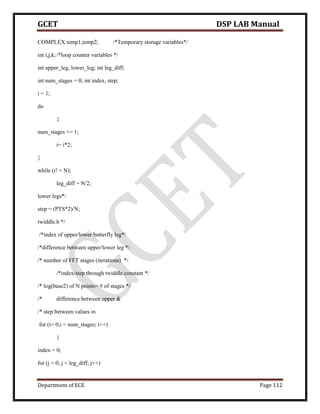
![GCET DSP LAB Manual
Department of ECE Page 113
{
/*for N-point FFT*/
for( upper_leg = j; upper_leg < N; upper_leg += (2*leg_diff))
{
lower_leg = upper_leg+leg_diff;
temp1.real = (Y[upper_leg]).real + (Y[lower_leg]).real;
temp1.imag = (Y[upper_leg]).imag + (Y[lower_leg]).imag;
temp2.real = (Y[upper_leg]).real - (y[lower_leg]).real;
temp2.imag = (Y[upper_leg]).imag - (Y[lower_leg]).imag;
(Y[lower_leg]).real = temp2.real*(w[index]).real
-temp2.imag*(w[index]).imag;
(Y[lower_leg]).imag = temp2.real*(w[index]).imag
+temp2.imag*(w[index]).real;
(Y[upper_leg]).real = temp1.real;
(Y[upper_leg]).imag = temp1.imag;
}
index += step;
}
leg_diff = leg_diff/2; step *= 2;
}
j = 0;
for (i= 1 ; i< (N-1 ); i++) /*bit reversal for resequencing data*/
{
k = N/2;
while (k <= j)](https://image.slidesharecdn.com/dsplab-200213145717/85/Dsp-lab-113-320.jpg)
![GCET DSP LAB Manual
Department of ECE Page 114
{
j= j - k;
k = k/2;
}
j= j + k;
if (i<j)
{
temp1.real = (Y[j]).real;
temp1.imag = (Y[j]).imag;
(Y[j]).real = (Y[i]).real;
(Y[j]).imag = (Y[i]).imag;
(Y[i]).real = temp1.real;
(Y(i]).imag = temp1.imag;
}
}
return;
}
PROCEDURE:
1 Open code composer studio, make sure the DSP kit is turned on.
2 Start a new project using ‘project-new’ pull down menu, save it in a separate directory
(c:ccstudiomyprojects) with the name ‘file name. pjt’.
3 Add the source file of linear convolution to the project using ‘project-add files to project’
pull down menu.
4 Add the linker command file ‘hello. cmd’ (cccstudiotutorialsdsk6713hello1hello.cmd)
5 Add the run time support library file rts6700.lib c-ccstudioc6000cgtoolslibrts6700.lib)
6 Compile program using the ‘project-compile’ pull down menu or by clicking the short cut
icon on the left side of program window.](https://image.slidesharecdn.com/dsplab-200213145717/85/Dsp-lab-114-320.jpg)