Downloaded 315 times

![Curtin University of Technology
Department of Petroleum Engineering
Master of Petroleum Engineering
Drilling Engineering
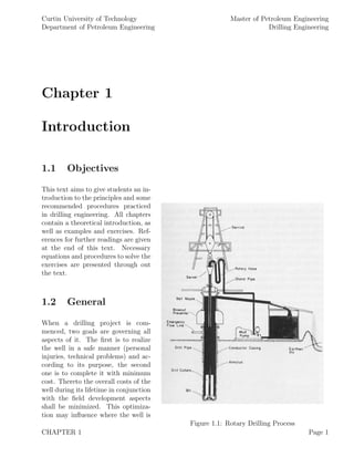
Derrick Man
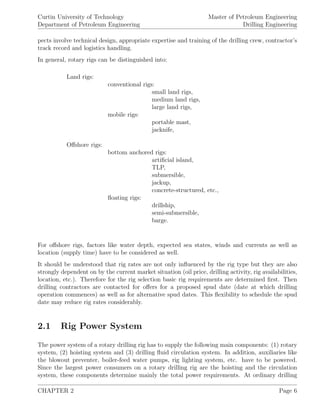
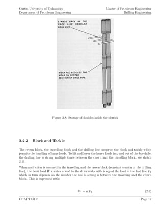
The derrickman works on the so-called monkeyboard, a small platform up in the derrick, usually
about 90 [ft] above the rotary table. When a connection is made or during tripping operations he
is handling and guiding the upper end of the pipe. During drilling operations the derrickman is
responsible for maintaining and repairing the pumps and other equipment as well as keeping tabs
on the drilling fluid.
Floor Men
During tripping, the rotary helpers are responsible for handling the lower end of the drill pipe as
well as operating tongs and wrenches to make or break a connection. During other times, they
also maintain equipment, keep it clean, do painting and in general help where ever help is needed.
Mud Engineer, Mud Logger
The service company who provides the mud almost always sends a mud engineer and a mud logger
to the rig site. They are constantly responsible for logging what is happening in the hole as well
as maintaining the propper mud conditions.
1.4 Miscellaneous
According to a wells final depth, it can be classified into:
Shallow well: < 2,000 [m]
Conventional well: 2,000 [m] - 3,500 [m]
Deep well: 3,500 [m] - 5,000 [m]
Ultra deep well: > 5,000 [m]
With the help of advanced technologies in MWD/LWD and extended reach drilling techniques
horizontal departures of 10,000+ [m] are possible today (Wytch Farm).
CHAPTER 1 Page 4](https://image.slidesharecdn.com/drillingengineering-160119095813/85/Drilling-engineering-12-320.jpg)
![Curtin University of Technology
Department of Petroleum Engineering
Master of Petroleum Engineering
Drilling Engineering
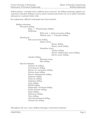
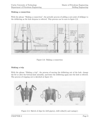
operations, the hoisting (lifting and lowering of the drillstring, casings, etc.) and the circulation
system are not operated at the same time. Therefore the same engines can be engaged to perform
both functions.
The power itself is either generated at the rig site using internal-combustion diesel engines, or
taken as electric power supply from existing power lines. The raw power is then transmitted to
the operating equipment via: (1) mechanical drives, (2) direct current (DC) or (3) alternating
current (AC) applying a silicon-controlled rectifier (SCR). Most of the newer rigs using the AC-
SCR systems. As guideline, power requirements for most rigs are between 1,000 to 3,000 [hp].
The rig power system’s performance is characterised by the output horsepower, torque and fuel
consumption for various engine speeds. These parameters are calculated with equations 2.1 to 2.4:
P =
ω.T
33, 000
(2.1)
Qi = 0.000393.Wf .ρd.H (2.2)
Et =
P
Qi
(2.3)
ω = 2.π.N (2.4)
where:
P [hp] ... shaft power developed by engine
ω [rad/min] ... angular velocity of the shaft
N [rev./min] ... shaft speed
T [ft-lbf] ... out-put torque
Qi [hp] ... heat energy consumption by engine
Wf [gal/hr] ... fuel consumption
H [BTU/lbm] ... heating value (diesel: 19,000 [BTU/lbm])
Et [1] ... overall power system efficiency
ρd [lbm/gal] ... density of fuel (diesel: 7.2 [lbm/gal])
33,000 ... conversion factor (ft-lbf/min/hp)
When the rig is operated at environments with non-standard temperatures (85 [F]) or at high
altitudes, the mechanical horsepower requirements have to be modified. This modification is
according to API standard 7B-11C:
(a) Deduction of 3 % of the standard brake horsepower for each 1,000 [ft] rise
CHAPTER 2 Page 7](https://image.slidesharecdn.com/drillingengineering-160119095813/85/Drilling-engineering-15-320.jpg)
![Curtin University of Technology
Department of Petroleum Engineering
Master of Petroleum Engineering
Drilling Engineering
in altitude above mean sea level,
(b) Deduction of 1 % of the standard brake horsepower for each 10 ◦
rise
or fall in temperature above or below 85 [F], respectively.
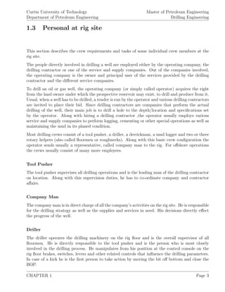
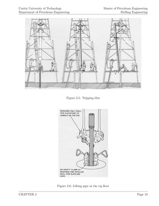
2.2 Hoisting System
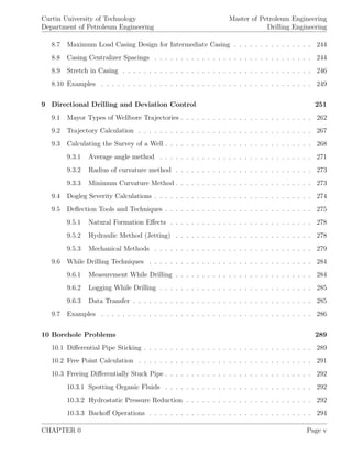
The main task of the hoisting system is to lower and raise the drillstring, casings, and other
subsurface equipment into or out of the well.
The hoisting equipment itself consists of: (1)draw works, (2) fast line, (3) crown block, (4) travel-
ling block, (5) dead line, (6) deal line anchor, (7) storage reel, (8) hook and (9) derrick, see sketch
2.2.
Figure 2.2: Hoisting system
CHAPTER 2 Page 8](https://image.slidesharecdn.com/drillingengineering-160119095813/85/Drilling-engineering-16-320.jpg)
![Curtin University of Technology
Department of Petroleum Engineering
Master of Petroleum Engineering
Drilling Engineering
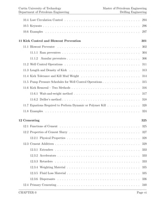
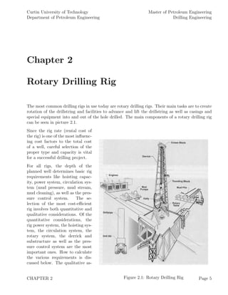
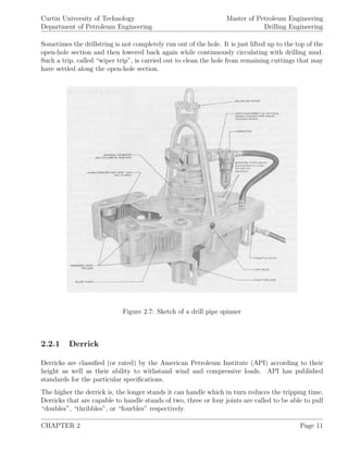
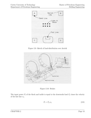
Figure 2.11: Block and tackle
The output power or “hook power” Ph is given by the hook load times the velocity of the travelling
block.
Ph = W.νb (2.7)
Figure 2.12: Efficiency factors for different tacklings
Drilling line:
The drilling line is a wire rope that is made of strands wounded around a steel core. It ranges in
diameter from 1
2
to 2 [in]. Its classification is based on the type of core, the number of strands
wrapped around the core, and the number of individual wires per strand. Examples of it can be
see in figure 2.13.
CHAPTER 2 Page 14](https://image.slidesharecdn.com/drillingengineering-160119095813/85/Drilling-engineering-22-320.jpg)
![Curtin University of Technology
Department of Petroleum Engineering
Master of Petroleum Engineering
Drilling Engineering
Figure 2.13: Drilling Line
Since the drilling line is constantly under biaxial load of tension and bending, its service life is
to be evaluated using a rating called “ton-mile”. By definition, a ton-mile is the amount of work
needed to move a 1-ton load over a distance of 1 mile.
When the drilling line has reached a specific ton-mile limit, which is mainly due to round trips,
setting casings, coring and drilling, it is removed from service. The ton-mile wear can be estimated
by:
Round Trip:
TR =
D. (Ls + D) .We
10, 560, 000
+
D. Wb + WC
2
2, 640, 000
(2.8)
where:
Wb [lb] ... effective weight of travelling assembly
Ls [ft] ... length of a drillpipe stand
We [lb/ft] ... effective weight per foot of drillpipe
D [ft] ... hole depth
WC [lb] ... effective weight of drill collar assembly
less the effective weight of the same length of drillpipe
It should be noted that the ton-miles are independent of the number of lines strung.
CHAPTER 2 Page 15](https://image.slidesharecdn.com/drillingengineering-160119095813/85/Drilling-engineering-23-320.jpg)
![Curtin University of Technology
Department of Petroleum Engineering
Master of Petroleum Engineering
Drilling Engineering
The ton-mile service of the drilling line is given for various activities according to:
Drilling operation: (drilling a section from depth d1 to d2) which accounts for:
1. drill ahead a length of kelly
2. pull up length of kelly
3. ream ahead a length of kelly
4. pull up a length of kelly
5. pull kelly in rathole
6. pick up a single (or double)
7. lower drill string in hole
8. pick up kelly and drill ahead
Td = 3. (TR at d2 − TR at d1) (2.9)
Coring operation: which accounts for:
1. core ahead a length of core barrel
2. pull up length of kelly
3. put kelly in rathole
4. pick up a single joint of drillpipe
5. lower drill string in hole
6. pick up kelly
Tc = 2. (TR2 − TR1) (2.10)
where:
TR2 [ton-mile] ... work done for one round trip at depth d2 where coring stopped
TR1 [tin-mile] ... work done for one round trip at depth d1 where coring started.
CHAPTER 2 Page 16](https://image.slidesharecdn.com/drillingengineering-160119095813/85/Drilling-engineering-24-320.jpg)
![Curtin University of Technology
Department of Petroleum Engineering
Master of Petroleum Engineering
Drilling Engineering
Running Casing:
Tsc = 0.5.
D. (Lcs + D) .Wcs
10, 560, 000
+
D.Wb
2, 640, 000
(2.11)
where:
Lcs [ft] ... length of casing joint
Wcs [lbm/ft] ... effective weight of casing in mud
The drilling line is subjected to most severe wear at the following two points:
1. The so called “pickup points”, which are at the top of the crown block sheaves and at the
bottom of the travelling block sheaves during tripping operations.
2. The so called “lap point”, which is located where a new layer or lap of wire begins on the
drum of the drawworks.
It is common practice that before the entire drilling line is replaced, the location of the pickup
points and the lap point are varied over different positions of the drilling line by slipping and/or
cutting the line.
A properly designed slipping-cut program ensures that the drilling line is maintained in good
condition and its wear is spread evenly over its length.
To slip the drilling line, the dead-line anchor has to be loosened and a few feet of new line is slipped
from the storage reel. Cutting off the drilling line requires that the line on the drawworks reel
is loosened. Since cutting takes longer and the drawworks reel comprise some additional storage,
the drilling line is usually slipped multiple times before it is cut. The length the drilling line is
slipped has to be properly calculated so that after slipping, the same part of the line, which was
used before at a pickup point or lap point, is not used again as a pickup point or lap point.
When selecting a drilling line, a “design factor” for the line is applied to compensate for wear
and shock loading. API’s recommendation for a minimum design factor (DF) is 3 for hoisting
operations and 2 for setting casing or pulling on stuck pipe operations. The design factor of the
drilling line is calculated by:
DF =
Nominal Strength of Wire Rope [lb]
Fast Line Load [lb]
(2.12)
CHAPTER 2 Page 17](https://image.slidesharecdn.com/drillingengineering-160119095813/85/Drilling-engineering-25-320.jpg)
![Curtin University of Technology
Department of Petroleum Engineering
Master of Petroleum Engineering
Drilling Engineering
Figure 2.14: Nominal breaking strength of 6 X 19 classification rope, bright (uncoated) or drawn-
galvanized wire, (IWRC)
2.2.3 Drawworks
The purpose of the drawworks is to provide the hoisting and breaking power to lift and lower the
heavy weights of drillstring and casings. The drawworks itself consists of: (1) Drum, (2) Brakes,
(3) Transmission and (4) Catheads, see figure 2.15.
The drum provides the movement of the drilling line which in turn lifts and lowers the travelling
block and consequently lifts or lowers the loads on the hook. The breaking torque, supplied by
the drum, has to be strong enough to be able to stop and hold the heavy loads of the drilling
line when lowered at high speed. The power required by the drawworks can be calculated when
considering the fast line load and fast line speed. In this way:
νf = n.νb (2.13)
Ph =
W.νb
33, 000.E
(2.14)
where:
Ph [hp] ... drum power output
νf [ft/min] ... velocity of the fast line
νb [ft/min] ... velocity of the travelling block
W [lb] ... hook load
CHAPTER 2 Page 18](https://image.slidesharecdn.com/drillingengineering-160119095813/85/Drilling-engineering-26-320.jpg)
![Curtin University of Technology
Department of Petroleum Engineering
Master of Petroleum Engineering
Drilling Engineering
n [1] ... number of lines strung
E [1] ... power efficiency of the block and tackle system
Figure 2.15: Drawworks
The input power to the drawworks is influenced by the efficiency of the chain drive and the shafts
inside the drawworks. This is expressed with:
E =
K. (1 − Kn
)
n. (1 − K)
(2.15)
where:
K [1] ... sheave and line efficiency, K = 0.9615 is an often used value.
When lowering the hook load, the efficiency factor and fast line load are determined by:
CHAPTER 2 Page 19](https://image.slidesharecdn.com/drillingengineering-160119095813/85/Drilling-engineering-27-320.jpg)
![Curtin University of Technology
Department of Petroleum Engineering
Master of Petroleum Engineering
Drilling Engineering
ELowering =
n.Kn
. (1 − K)
1 − Kn
(2.16)
Ff−Lowering =
W.K−n
. (1 − K)
1 − Kn
(2.17)
where:
Ff [lbf] ... tension in the fast line
2.3 Rig Selection
Following parameters are used to determine the minimum criteria to select a suitable drilling rig:
(1) Static tension in the fast line when upward motion is impending
(2) Maximum hook horsepower
(3) Maximum hoisting speed
(4) Actual derrick load
(5) Maximum equivalent derrick load
(6) Derrick efficiency factor
They can be calculated by following equations:
Pi = Ff .νf (2.18)
νb =
Ph
W
(2.19)
Fd =
1 + E + E.n
E.n
.W (2.20)
Fde =
n + 4
n
.W (2.21)
Ed =
Fd
Fde
=
E.(n + 1) + 1
E.(n + 4)
(2.22)
where:
CHAPTER 2 Page 20](https://image.slidesharecdn.com/drillingengineering-160119095813/85/Drilling-engineering-28-320.jpg)
![Curtin University of Technology
Department of Petroleum Engineering
Master of Petroleum Engineering
Drilling Engineering
Fd [lbf] ... load applied to derrick, sum of the hook load,
tension in the dead line and tension in the fast line
Fde [lbf] ... maximum equivalent derrick load, equal to
four times the maximum leg load
Ed [1] ... derrick efficiency factor
CHAPTER 2 Page 21](https://image.slidesharecdn.com/drillingengineering-160119095813/85/Drilling-engineering-29-320.jpg)
![Curtin University of Technology
Department of Petroleum Engineering
Master of Petroleum Engineering
Drilling Engineering
Figure 2.18: Mixing hopper
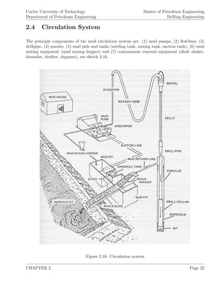
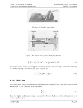
2.4.1 Mud Pumps
Nowadays there are two types of mud pumps in use (duplex pump, triplex pump), both equipped
with reciprocating positive-displacement pistons. The amount of mud and the pressure the mud
pumps release the mud to the circulation system are controlled via changing of pump liners and
pistons as well as control of the speed [stroke/minute] the pump is moving.
Duplex Mud Pump
The duplex mud pump consists of two cylinders and is double-acting. This means that drilling
mud is pumped with the forward and backward movement of the barrel. The pump displacement
on the forward movement of the piston is given by:
Ffd =
π
4
.d2
l .Ls (2.23)
On the backward movement of the piston, the volume is displaced:
π
4
.d2
l .Ls −
π
4
.d2
r.Ls =
π
4
.(d2
l − d2
r).Ls (2.24)
Thus the total displacement per complete pump cycle is:
CHAPTER 2 Page 24](https://image.slidesharecdn.com/drillingengineering-160119095813/85/Drilling-engineering-32-320.jpg)
![Curtin University of Technology
Department of Petroleum Engineering
Master of Petroleum Engineering
Drilling Engineering
Fp =
3.π
4
.Ls.d2
l .Ev (2.28)
where:
Fp [in2
/cycle] ... pump displacement (also called “pump factor”)
Ev [1] ... volumetric efficiency (90 ÷ 100 %)
Ls [in] ... stroke length
dr [in] ... piston rod diameter
dl [in] ... liner diameter
Figure 2.21: Triplex mud pump
Figure 2.22: Triplex mud pump - Pumping Scheme
The triplex pumps are generally lighter and more compact than the duplex pumps and their
output pressure pulsations are not as large. Because of this and since triplex pumps are cheaper
to operate, modern rigs are most often equipped with triplex mud pumps.
The the flow rate of the pump [in2
/min] can be calculated with:
CHAPTER 2 Page 26](https://image.slidesharecdn.com/drillingengineering-160119095813/85/Drilling-engineering-34-320.jpg)
![Curtin University of Technology
Department of Petroleum Engineering
Master of Petroleum Engineering
Drilling Engineering
q = N.Fp (2.29)
where:
N [cycles/min] ... number of cycles per minute
The overall efficiency of a mud pump is the product of the mechanical and the volumetric efficiency.
The mechanical efficiency is often assumed to be 90% and is related to the efficiency of the prime
mover itself and the linkage to the pump drive shaft. The volumetric efficiency of a mud pump
with adequately charged suction system can be as high as 100%. Therefore most manufactures
rate their pumps with a total efficiency of 90% (mechanical efficiency: 90%, volumetric efficiency:
100%).
Note that per revolution, the duplex pump makes two cycles (double-acting) where the triplex
pump completes one cycle (single-acting).
The terms “cycle” and “stroke” are applied interchangeably in the industry and refer to one
complete pump revolution.
Pumps are generally rated according to their:
1. Hydraulic power,
2. Maximum pressure,
3. Maximum flow rate.
Since the inlet pressure is essentially atmospheric pressure, the increase of mud pressure due to
the mud pump is approximately equal the discharge pressure.
The hydraulic power [hp] provided by the mud pump can be calculated as:
PH =
∆p.q
1, 714
(2.30)
where:
∆p [psi] ... pump discharge pressure
q [gal/min] ... pump discharge flow rate
CHAPTER 2 Page 27](https://image.slidesharecdn.com/drillingengineering-160119095813/85/Drilling-engineering-35-320.jpg)
![Curtin University of Technology
Department of Petroleum Engineering
Master of Petroleum Engineering
Drilling Engineering
At a given hydraulic power level, the maximum discharge pressure and the flow rate can be varied
by changing the stroke rate as well as the liner seize. A smaller liner will allow the operator to
obtain a higher pump pressure but at a lower flow rate. Pressures above 3,500 [psi] are applied
seldomly since they cause a significant increase in maintenance problems.
In practice, especially at shallow, large diameter section, more pumps are often used simultaneously
to feed the mud circulation system with the required total mud flow and intake pressure. For this
reason the various mud pumps are connected in parallel and operated with the same output
pressure. The individual mud streams are added to compute the total one.
Between the mud pumps and the drillstring so called “surge chambers”, see figure 2.23, are
installed. Their main task is to dampen the pressure pulses, created by the mud pumps.
Figure 2.23: Surge chamber
Furthermore a “discharge line” containing a relief valve is assembled before the mud reaches the
stand pipe, thus in case the pump is started against a closed valve, line rapture is prevented.
When the mud returns to the surface, it is lead over shale shakers that are composed of one or
more vibrating screens over which the mud passes before it is feed to the mud pits.
The mud pits are required to hold an excess mud volume at the surface. Here fine cuttings can
settle and gas, that was not mechanically separated can be released further. In addition, in the
event of lost circulation, the lost mud can be replaced by mud from the surface pits.
CHAPTER 2 Page 28](https://image.slidesharecdn.com/drillingengineering-160119095813/85/Drilling-engineering-36-320.jpg)
![Curtin University of Technology
Department of Petroleum Engineering
Master of Petroleum Engineering
Drilling Engineering
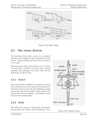
2.5.3 Rotary Drive
The rotary drive consists of master pushing and kelly pushing. The master pushing receives its
rotational momentum from the compound and drives the kelly pushing which in turn transfers
the rotation to the kelly.
Figure 2.27: Master and kelly pushing
Following equation can be applied to calculate the rotational power that is induced to the drill-
string:
PR =
T.N
5, 250
(2.31)
where:
PR [hp] ... rotational power induced to the drillstring
T [ft-lb] ... rotary torque induced to the drillstring
N [rpm] ... rotation speed
Prior to drilling, the estimation of induced rotational torque is difficult since it comprises a com-
bination of the torque at the bit as well as torque losses at the drillstring, following empirical
relation has been developed:
CHAPTER 2 Page 31](https://image.slidesharecdn.com/drillingengineering-160119095813/85/Drilling-engineering-39-320.jpg)
![Curtin University of Technology
Department of Petroleum Engineering
Master of Petroleum Engineering
Drilling Engineering
PR = F.N (2.32)
The torque factor is approximated with 1.5 for wells with MD smaller than 10,000 [ft], 1.75 for
wells with MD of 10,000 to 15,000 [ft] and 2.0 for wells with MD larger than 15,000 [ft].
The volume contained and displaced by the drillstring can be calculated as:
Capacity of drillpipe or drill collar:
Vp =
d2
1, 029.4
(2.33)
Capacity of the annulus behind drillpipe or drill collar:
Va =
(d2
2 − d2
1)
1, 029.4
(2.34)
Displacement of drillpipe or drill collar:
Vs =
(d2
1 − d2
)
1, 029.4
(2.35)
where:
d [in] ... inside diameter of drillpipe or drill collar
d1 [in] ... outside diameter of drillpipe or drill collar
d2 [in] ... hole diameter
V [bbl/ft] ... capacity of drillpipe, collar or annulus
2.6 Drilling Cost Analysis
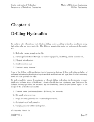
To estimate the cost of realizing a well as well as to perform economical evaluation of the drilling
project, before commencing the project, a so called AFE (Authority For Expenditure) has to be
prepared and signed of by the operator. Within the AFE all cost items are listed as they are
known or can be estimated at the planning stage. During drilling, a close follow up of the actual
cost and a comparison with the estimated (and authorized) ones are done on a daily bases.
When preparing an AFE, different completions and objectives (dry hole, with casing and comple-
tion, etc) can be included to cost-estimate different scenarios.
Generally, an AFE consists of the following major groups:
CHAPTER 2 Page 32](https://image.slidesharecdn.com/drillingengineering-160119095813/85/Drilling-engineering-40-320.jpg)
![Curtin University of Technology
Department of Petroleum Engineering
Master of Petroleum Engineering
Drilling Engineering
(1) Wellsite preparation,
(2) Rig mobilization and rigging up,
(3) Rig Rental,
(4) Drilling Mud,
(5) Bits and Tools,
(6) Casings,
(7) Formation evaluation
The listed cost items and their spread are different at each company and can be different within
one company (onshore-offshore, various locations, etc.).
Along with the well plan (well proposal) a operational schedule as well as a schedule of expected
daily costs has to be prepared.
In the following simple methods to estimate the drilling costs as well as, the drilling and tripping
times are given.
2.6.1 Drilling Costs
On of the most basic estimations of drilling costs is given by:
Cf =
Cb + Cr (tb + tc + tt)
D
(2.36)
where:
Cf [$/ft] ... cost per unit depth
Cb [$] ... cost of bit
Cr [$/hr] ... fixed operating cost of rig per unit time
D [ft] ... depth drilled
tb [hr] ... total rotation time during the bit run
tc [hr] ... total non-rotating time during the bit run
tt [hr] ... trip time
It has been found that drilling cost generally tend to increase exponentially with depth. Thus,
when curve-fitting and correlation methods are applied, it is convenient to assume a relationship
between drilling cost C and depth D as in equation 2.37:
C = a.eb.D
(2.37)
The constants a and b depend primary on the well location.
CHAPTER 2 Page 33](https://image.slidesharecdn.com/drillingengineering-160119095813/85/Drilling-engineering-41-320.jpg)
![Curtin University of Technology
Department of Petroleum Engineering
Master of Petroleum Engineering
Drilling Engineering
2.6.2 Drilling Time
The drilling time can be estimated based on experience and historical penetration rates. Note that
the penetration rate depends on: (1) type of bit used, (2) wear of bit used, (3) drilling parameters
applied (WOB, RPM), (4) hydraulics applied (hydraulic impact force due to mud flow through
nozzles), (5) effectiveness of cuttings removal, (6) formation strength and (7) formation type.
Therefore an analytic prediction of the rate of penetration (ROP) is impossible. Estimations are
generally based on the assumption of similar parameters and historic ROPs.
To estimate the drilling time, the so called “penetration rate equation”, equation 2.38, is analyzed.
dD
dt
= K.ea2.D
(2.38)
When the historical values of depth [ft] versus ROP [ft/hr] are plotted on a semilogarithmic graph
paper (depth on linear scale), a straight line best-fit of the equation:
td =
1
2.303.a2.K
.e2.203.a2.D
(2.39)
estimates the drilling time. Here a2 is the reciprocal of the change in depth per log cycle of the
fitted straight line, K is the value of ROP at the surface (intercept of fitted straight line at depth
= 0 ft).
The depth that can be drilled with each individual bit depends on (1) bit condition when inserted,
(2) drilling parameters, (3) rock strength and (4) rock abrasiveness. Estimations of possible
footages between trips can be obtained from historical data or applying equation 2.40:
D =
1
2.303.a2
.ln 2.303a2.L.tb + 22.303.a2.Di
(2.40)
where:
Di [ft] ... depth of the last trip
D [ft] ... depth of the next trip
All other parameters are defined as above.
2.6.3 Tripping Time
Tripping time is also a major contributor to the total time spent for drilling a well. Tripping can
be either scheduled (change of bit, reach of casing point, scheduled well-cleaning circulation) or
CHAPTER 2 Page 34](https://image.slidesharecdn.com/drillingengineering-160119095813/85/Drilling-engineering-42-320.jpg)
![Curtin University of Technology
Department of Petroleum Engineering
Master of Petroleum Engineering
Drilling Engineering
on-scheduled, due to troubles. Types of troubles, their origin and possible actions are discussed
in a later chapter.
Following relationship can be applied to estimate the tripping time to change the bit. Thus the
operations of trip out, change bit, trip in are included:
tt = 2.
ts
ls
.D (2.41)
where:
tt [hr] ... required time for round trip
ts [hr] ... average time required to handle one stand
D [ft or m] ... length of drillstring to trip
ls [ft or m] ... average length of one stand
The term “stand” refers to the joints of drillpipe left connected and placed inside the derrick
during tripping. Depending on the derrick seize, one stand consists mostly of three, sometimes
four drillpipes. In this way during tripping only each third (fourth) connection has to be broken
and made up for tripping.
CHAPTER 2 Page 35](https://image.slidesharecdn.com/drillingengineering-160119095813/85/Drilling-engineering-43-320.jpg)
![Curtin University of Technology
Department of Petroleum Engineering
Master of Petroleum Engineering
Drilling Engineering
2.7 Examples
1. The output torque and speed of a diesel engine is 1,650 [ft-lbf] and 800 [rpm] respectively.
Calculate the brake horsepower and overall engine efficiency when the diesel consumption rate is
15.7 [gal/hr]. What is the fuel consumption for a 24 hr working day?
2. When drilling at 7,000 [ft] with an assembly consisting of 500 [ft] drill collars (8 [in] OD, 2.5
[in] ID, 154 [lbm/ft]) on a 5 [in], 19.5 [lbm/ft] , a 10.0 [ppg] drilling mud is used. What are the
ton-miles applying following assumptions (one joint of casing is 40 [ft], travelling block assembly
weights 28,000 [lbm], each stand is 93 [ft] long) when:
(a) Running 7 [in], 29 [lbm/ft] casing,
(b) Coring from 7,000 [ft] to 7,080 [ft],
(c) Drilling from 7,000 [ft] to 7,200 [ft],
(d) Making a round-trip at 7,000 [ft]?
3. The rig’s drawworks can provide a maximum power of 800 [hp]. To lift the calculated load of
200,000 [lb], 10 lines are strung between the crown block and the traveling block. The lead line is
anchored to a derrick leg on one side of the v-door. What is the:
(a) Static tension in the fast line,
(b) Maximum hook horsepower available,
(c) Maximum hoisting speed,
(d) Derrick load when upward motion is impending,
(e) Maximum equivalent derrick load,
(f) Derrick efficiency factor?
4. After circulation the drillstring is recognized to be stuck. For pulling the drillstring, following
equipment data have to be considered: derrick can support a maximum equivalent derrick load of
500,000 [lbf], the drilling line strength is 51,200 [lbf], the maximum tension load of the drillpipe
is 396,000 [lbf]. 8 lines are strung between the crown block and the traveling block, for pulling to
free the stuck pipe, a safety factor of 2.0 is to be applied for the derrick, the drillpipe as well as
the drilling line. What is the maximum force the driller can pull to try to free the pipe?
5. To run 425,000 [lb] of casing on a 10-line system, a 1.125 [in], 6x19 extra improved plow steel
drilling line is used. When K is assumed to be 0.9615, does this configuration meet a safety factor
requirement for the ropes of 2.0? What is the maximum load that can be run meeting the safety
factor?
CHAPTER 2 Page 36](https://image.slidesharecdn.com/drillingengineering-160119095813/85/Drilling-engineering-44-320.jpg)
![Curtin University of Technology
Department of Petroleum Engineering
Master of Petroleum Engineering
Drilling Engineering
6. A drillstring of 300,000 [lb] is used in a well where the rig has sufficient horsepower to run
the string at a minimum rate of 93 [ft/min]. The hoisting system has 8 lines between the crown
block and the travelling block, the mechanical drive of the rig has following configuration: Engine
no. 1: (4 shafts, 3 chains), engine no. 2: (5 shafts, 4 chains), engine no. 3: (6 shafts, 5 chains).
Thus the total elements of engine 1 is 7, of engine 2 9 and of engine 3 11. When the efficiencies of
each shaft, chain and sheave pair is 0.98 and 0.75 for the torque converter, what is the minimum
acceptable input horsepower and fast line velocity?
7. A triplex pump is operating at 120 [cycles/min] and discharging the mud at 3,000 [psig]. When
the pump has installed a 6 [in] liner operating with 11 [in] strokes, what are the:
(a) Pump factor in [gal/cycles] when 100 %
volumetric efficiency is assumed,
(b) Flow rate in [gal/min],
(c) Pump power development?
8. A drillstring consists of 9,000 [ft] 5 [in], 19,5 [lbm/ft] drillpipe, and 1,000 [ft] of 8 [in] OD, 3
[in] ID drill collars. What is the:
(a) Capacity of the drillpipe in [bbl],
(b) Capacity of the drill collars in [bbl],
(c) Number of pump cycles required to pump surface mud to the bit
(duplex pump, 6 [in] liners, 2.5 [in] rods, 16 [in] strokes,
pumping at 85 % volumetric efficiency),
(d) Displacement of drillpipes in [bbl/ft],
(e) Displacement of drill collars in [bbl/ft],
(f) Loss in fluid level in the hole if 10 stands (thribbles) drillpipe
are pulled without filling the hole (casing 10.05 [in] ID),
(g) Change in fluid level in the pit when the hole is filled after
pulling 10 stands of drillpipe. The pit is 8 [ft] wide and
20 [ft] long.
9. A diesel engine gives an output torque of 1,740 [ft-lbf] at an engine speed of 1,200 [rpm]. The
rig is operated in Mexico at an altitude of 1,430 [ft] above MSL at a average temperature of 28
◦
C. When the fuel consumption rate is 31.8 [gal/hr], what is the output power and the overall
efficiency of the engine?
10. A rig must hoist a load of 320,000 [lb]. The drawworks can provide an input power to the
block and tackle system as high as 500 [hp]. Eight lines are strung between the crown block and
the travelling block. Calculate:
CHAPTER 2 Page 37](https://image.slidesharecdn.com/drillingengineering-160119095813/85/Drilling-engineering-45-320.jpg)
![Curtin University of Technology
Department of Petroleum Engineering
Master of Petroleum Engineering
Drilling Engineering
(a) Static tension in the fast line,
(b) Maximum hook horse power,
(c) Maximum hoisting speed,
(d) Effective derrick load,
(e) Maximum equivalent derrick load,
(f) Derrick efficiency factor.
11. The weight of the travelling block and hook is 23,500 [lb], the total well depth equals 10,000
[ft]. A drillpipe of OD 5 [in], ID 4.276 [in], 19.5 [lb/ft] and 500 [ft] of drill collar OD 8 [in], ID 2-13
16
[in], 150 [lb/ft] comprise the drillstring. The hole was drilled with a mud weight of 75 [lb/ft3
]. steel
weight: 489.5 [lb/ft3
], line and sheave efficiency factor = 0.9615, block and tackle efficiency=0.81.
Calculate:
(a) Weight of the drill string in air and in mud,
(b) Hook load,
(c) Dead line and fast line load,
(d) Dynamic crown load,
(e) Design factor for wire line for running drill string,
CHAPTER 2 Page 38](https://image.slidesharecdn.com/drillingengineering-160119095813/85/Drilling-engineering-46-320.jpg)
![Curtin University of Technology
Department of Petroleum Engineering
Master of Petroleum Engineering
Drilling Engineering
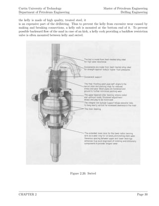
Figure 3.1: Pore pressure and fracture gradient profile
for different offshore rigs (semisub and jackup)
Correct RKB to MSL reference:
dMSL = dRKB.
D
D − hRKB
(3.1)
Convert MSL data to RKB:
dRKB = dMSL.
D − hRKB
D
(3.2)
Another common problem is when data
referenced to one RKB (e.g. rig used
to drill the wildcat well) has to be ap-
plied for further/later calculations (e.g.
drilling development wells from a pro-
duction platform). Here the data have
to be corrected from RKB1 to RKB2 .
Correct from RKB1 to RKB2:
dRKB2 = dRKB1 .
D − ∆h
D
(3.3)
where:
D [m or ft] ... total depth of point of interest in reference to RKB
hRKB [m or ft] ... height of RKB above MSL
∆h [m or ft] ... difference of elevation of RKB1 to RKB2
CHAPTER 3 Page 40](https://image.slidesharecdn.com/drillingengineering-160119095813/85/Drilling-engineering-48-320.jpg)
![Curtin University of Technology
Department of Petroleum Engineering
Master of Petroleum Engineering
Drilling Engineering
ρfl [ppg] ... density of the fluid causing hydrostatic pressure
ρ [kg/m3
] ... average fluid density
D [ft] ... depth at which hydrostatic pressure occurs (TVD)
h [m] ... vertical height of column of liquid
p [psi] ... hydrostatic pressure
g [m/s2
] ... acceleration due to gravity
Figure 3.3: Seismic record to determine the subsurface structure
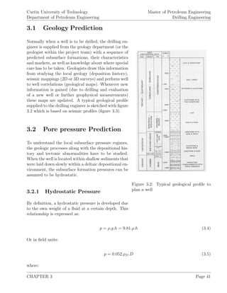
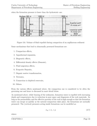
When the weight of the solid particles buried are supported by grain-to-grain contacts and the with
the particles buried water has free hydraulic contact to the surface, the formation is considered
as hydrostatically pressured. As it can be seen, the formation pressure, when hydrostatically
pressured, depends only on the density of the formation fluid (usually in the range of 1.00 [g/cm3
]
to 1.08 [g/cm3
], see table 3.4) and the depth in TVD.
CHAPTER 3 Page 42](https://image.slidesharecdn.com/drillingengineering-160119095813/85/Drilling-engineering-50-320.jpg)
![Curtin University of Technology
Department of Petroleum Engineering
Master of Petroleum Engineering
Drilling Engineering
σob [psi] ... overburden stress
σz [psi] ... vertical stress supported by the grain-to-grain connections
p [psi] ... formation pore pressure
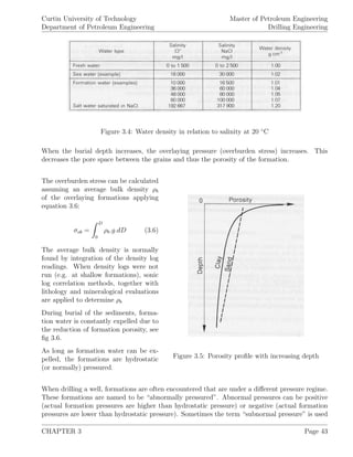
When the formation water can not escape as quickly as the pore space is reduced, it is trapped
inside the formations. In this scenario, the increasing overburden stress will pressurize the forma-
tion water and the formation will become abnormally pressured. In this situation, the porosity
of the formation will not follow the natural compaction trend (porosity at abnormally pressured
formations will be higher than at normally pressured ones). Along with the higher porosity, the
bulk density as well as the formation resistivity will be lower at abnormally pressured formations.
These circumstances are often applied to detect and estimate the abnormal formation pressures.
The bulk density [ppg] of a formation is estimated by equation 3.8:
ρb = ρg.(1 − φ) + ρfl.φ (3.8)
where:
ρg [ppg] ... grain density
ρfl [ppg] ... formation fluid density
φ [1] ... total porosity of the formation
Figure 3.7: Average bulk density change in sediments
As it can be seen from figure 3.7, an average bulk density of 2.31 [g/cm3] (equal to 1 [psi/ft]) can
be assumed for deep wells as approximation.
CHAPTER 3 Page 45](https://image.slidesharecdn.com/drillingengineering-160119095813/85/Drilling-engineering-53-320.jpg)
![Curtin University of Technology
Department of Petroleum Engineering
Master of Petroleum Engineering
Drilling Engineering
In areas of frequent drilling activities or where formation evaluation is carried out extensively, the
natural trend of bulk density change with depth is known.
For shale formations that follow the natural compaction trend, it has been observed that the
porosity change with depth can be described using below relationship:
φ = φo.e−K.Ds
(3.9)
where:
φ [1] ... porosity at depth of interest
φo [1] ... porosity at the surface
K [ft−1
] ... porosity decline constant, specific for each location
Ds [ft] ... depth of interest (TVD)
When equation 3.9 is substituted in equation 3.8 and equation 3.6 and after integration the
overburden stress profile is found for an offshore well as:
σob = 0.052.ρsw.Dw + 0.052.ρg.Dg −
0.052
K
.(ρg − ρfl).φo.(1 − e−K.Dg
) (3.10)
where:
Dg [ft] ... depth of sediment from sea bottom
ρsw [ppg] ... sea water density
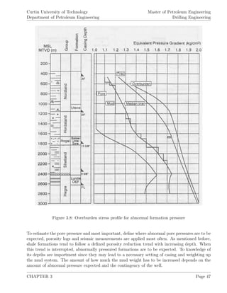
Thus when the overburden stress profile is known, the depth where the abnormal pressure starts
is given and with the shape of the profile, it is determined at which depth the matrix stress is
equal to the matrix stress at the abnormal formation pressure (“matrix point”), see figure 3.8.
Now, the normal formation pressure at the matrix point is calculated by equation 3.5 and the
matrix stress with equation 3.7. Applying the assumption that the matrix stress is equal at the
matrix point with the one at the abnormal formation pressure, and when the overburden stress
at the abnormal formation pressure is calculated with equation 3.10, the abnormal formation
pressure is found when rearranging equation 3.7.
The actual measurement of formation pore pressure is very expensive and possible only after the
formations have been drilled. In this respect, pore pressures have to be estimated before drilling to
properly plan the mud weights, casing setting depths, casing design, etc. as well as being closely
monitored during drilling.
CHAPTER 3 Page 46](https://image.slidesharecdn.com/drillingengineering-160119095813/85/Drilling-engineering-54-320.jpg)
![Curtin University of Technology
Department of Petroleum Engineering
Master of Petroleum Engineering
Drilling Engineering
Abnormal pressure detection while drilling
When the well is in progress and abnormal formation pressures are expected, various parameters
are observed and cross-plotted. Some of these while drilling detection methods are:
(a) Penetration rate,
(b) “d” exponent,
(c) Sigmalog,
(d) Various drilling rate normalisations,
(e) Torque measurements,
(f) Overpull and drag,
(g) Hole fill,
(h) Pit level – differential flow – pump pressure,
(i) Measurements while drilling,
(j) Mud gas,
(k) Mud density,
(l) Mud temperature,
(m) Mud resistivity,
(n) Lithology,
(o) Shale density,
(p) Shale factor (CEC),
(q) Shape, size and abundance of cuttings,
(r) Cuttings gas,
(s) X-ray diffraction,
(t) Oil show analyzer,
(u) Nuclear magnetic resonance.
d-exponent
It has been observed that when the same formation is drilled applying the same drilling parameters
(WOB, RPM, hydraulics, etc.), a change in rate of penetration is caused by the change of differ-
ential pressure (borehole pressure - formation pressure). Here an increase of differential pressure
(a decrease of formation pressure) causes a decrease of ROP, a decrease of differential pressure (in-
crease of formation pressure) an increase of ROP. Applying this observation to abnormal formation
pressure detection, the so called “d-exponent” was developed.
d =
log10
R
60.N
log10
12.W
106.D
(3.11)
where:
R [ft/hr] ... penetration rate
N [rev./min] ... rotation speed
CHAPTER 3 Page 48](https://image.slidesharecdn.com/drillingengineering-160119095813/85/Drilling-engineering-56-320.jpg)
![Curtin University of Technology
Department of Petroleum Engineering
Master of Petroleum Engineering
Drilling Engineering
W [lb] ... weight on bit
D [in] ... hole seize
The term R
60.N
is always less than 1 and represents penetration in feet per drilling table rotation.
Wile drilling is in progress, a d-exponent log is been drawn. Any decrease of the d-exponent value
in an argillaceous sequence is commonly interpreted with the respective degree of undercompaction
and associated with abnormal pressure. Practice has shown that the d-exponent is not sufficient to
conclude for abnormal pressured formations. The equation determining the d-exponent assumes
a constant mud weight. In practice, mud weight is changed during the well proceeds. Since a
change in mud weight results in a change of d-exponent, a new trend line for each mud weight has
to be established, which needs the drilling of a few tenth of feet. To account for this effect, the so
called “corrected d-exponent” dc was developed:
dc = d.
ρfl
ρeqv
(3.12)
where:
d ... d-exponent calculated with equation 3.11
ρfl [ppg] ... formation fluid density for the hydrostatic gradient in the region
ρeqv [ppg] ... mud weight
Abnormal pressure evaluation
After an abnormal pressure is detected or the well is completed, various wireline log measurements
are used to evaluate the amount of overpressures present. Among the most common ones are:
(a) Resistivity, conductivity log,
(b) Sonic log,
(c) Density log,
(d) Neutron porosity log,
(e) Gamma ray, spectrometer,
(f) Velocity survey or checkshot,
(g) Vertical seismic profile.
With these log measurements trend lines are established and the amount the values deviate at
the abnormally pressured formations from the trend line are applied to determine the value of
overpressure. Sketches of how deviations of the trend lines for the individual wireline logs are
shown in figure 3.9.
Methods to evaluate the amount of overpressures are:
CHAPTER 3 Page 49](https://image.slidesharecdn.com/drillingengineering-160119095813/85/Drilling-engineering-57-320.jpg)

![Curtin University of Technology
Department of Petroleum Engineering
Master of Petroleum Engineering
Drilling Engineering
data into two groups, one concerning the competent shale formations with higher fracture gradients
and a second one for permeable sandstone (coal, chalk, etc.) formations exhibiting weaker fracture
gradients.
When LOT data are evaluated, a considerable spread is often found. It is common practice to
first plot the LOT values vs. depth and check how well they correlate. When the spread of LOT
values is to large to define a correlation line, the “effective stress concept” can be applied.
Effective stresses
The effective stress concept states that the stress in the rock matrix is equal the total stress minus
the pore pressure. This is expressed in equation 3.13:
σeff = σt − Po (3.13)
Horizontal stresses
When the borehole is vertical, as well as a hydrostatic stress state is assumed, the LOT values
can be expressed as:
LOT = 2.σa − Po (3.14)
where:
LOT [psi] ... leak-off test value
σa [psi] ... average horizontal stress
Po [psi] ... pore pressure
Since when the LOT is carried out, the pore pressure is known or measured as well, the horizontal
stress can be evaluated by equation 3.15:
σa =
LOT − Po
2
(3.15)
The horizontal stress as derived above can also be used for a correlation when plotted vs. depth.
Influence of hole inclination
Since formations are generally not isotropic or even under a hydrostatic stress state which was
assumed above, fracture gradients do normally depend on the inclination of the borehole. To
account for this, the coupling of the fracture gradient of an inclined hole with a vertical one can
be modeled by equation 3.16:
CHAPTER 3 Page 51](https://image.slidesharecdn.com/drillingengineering-160119095813/85/Drilling-engineering-59-320.jpg)
![Curtin University of Technology
Department of Petroleum Engineering
Master of Petroleum Engineering
Drilling Engineering
Pwf (θ) = Pwf (0) +
1
3
.(Po − P∗
o ). sin2
θ (3.16)
where:
Pwf (θ) [psi] ... fracture gradient at α inclined borehole
Pwf (0) [psi] ... fracture gradient at vertical borehole
Po [psi] ... pore pressure at specific depth
P∗
o [psi] ... pore pressure constant
θ [rad] ... borehole inclination
Fracture gradients at shallow depth
The determination of fracture gradients for shallow depth is often difficult since very little data
exists. This is due to the circumstance that at shallow depth, blowout preventers are often
not installed and thus no pressure testing can be carried out. Especially at offshore wells, the
knowledge of shallow fracture gradients are important since the margin between pore pressure and
fracture gradient is narrow and the danger of shallow gas pockets exists. As practice shows, the
spread of fracture gradients are larger at shallow depths and decrease with depth.
3.4 Mud Weight Planning
Selecting the correct mud weight for drilling the individual sections comprises a key factor to
realize a in-gauge hole and avoid various borehole problems.
Too low mud weight may result in collapse and fill problems (well cleaning), while too high mud
weight may result in mud losses or pipe sticking. Practice has also shown that excessive variations
in mud weight may lead to borehole failure (fatigue type effect), thus a more constant mud weight
program should be aimed for. Along with a more constant mud weight program, the equivalent
circulation density (ECD) as well as the surge and swab pressures shall be kept within limits.
Washouts of the borehole are sometimes caused by jet actions of the bit nozzles but also sometimes
by to low mud weight causing a breakdown of the borehole wall. A higher mud weight will therefore
balance the rock stresses better and tend to keep the borehole more in-gauge.
A decease in hole diameter is often due to swelling (clay swelling) requiring wiper trips or back-
reaming. This necessity is sometimes reduced by higher mud weights.
An increased mud weight increases the danger of becoming differential stuck at permeable for-
mations. Therefore mud weight shall not be chosen to be to high. However, what is sometimes
believed to be a differentially stuck drillstring is sometimes due to a borehole collapse which packs
the hole around the bottom-hole assembly. A lower mud weight also causes breakouts of shale
layers leaving sand formations in-gauge, see figure 3.10. This can increase the danger of getting
differential stuck at the exposed sand stringers.
CHAPTER 3 Page 52](https://image.slidesharecdn.com/drillingengineering-160119095813/85/Drilling-engineering-60-320.jpg)
![Curtin University of Technology
Department of Petroleum Engineering
Master of Petroleum Engineering
Drilling Engineering
Thus when considering the danger of differential sticking, it is recommended to keep the mud
weight below a certain value but it shall not be as low as possible.
Figure 3.10: Partial collapse in mixed lithology
The same is true for lost circulation problems.
As long as the mud weight is kept below a
critical value, lost circulation will not occur.
It is often argued that to have a as high as
possible rate of penetration, the mud weight
shall be kept as close as possible to the for-
mation pressure gradient plus a safety mar-
gin of around 100 [psi]. Although it is true
that a small reduction in mud weight increases
the penetration rate, but this increases has to
be weighted against the possible induction of
hole problems and additional lost time.
A higher mud weight requires the use of more
mud additives which makes the well more ex-
pensive, but it was found that these extra costs are usually neglectable.
When drilling within areas where the subsurface pressure regimes are not well known, it is often
argued that a lower mud weight easies the detection of abnormal pressures. In some locations, a
practice called “drilling for a kick” was applied to detect overpressured formations. For this, a
relatively low mud weight was applied until a kick was detected (pressure gradient at this depth
was equal to the used mud weight) and handling the kick, the mud weight was increased. Therefore
and since a higher mud weight also suppresses high gas readings, the mud weight of exploration
wells are often designed to be lighter than the ones for development wells.
Figure 3.11: Effects of varying the borehole pressure
Based on all these considera-
tions, the “median line con-
cept” is recommended gen-
erally for mud weight plan-
ning.
Thereto, the mid-point be-
tween the fracture pressure
and the pore pressure defines
the borehole pressure that
is equal to the ideal in-situ
stress. Maintaining the mud
pressure close to this level
causes least disturbances on
the borehole wall.
CHAPTER 3 Page 53](https://image.slidesharecdn.com/drillingengineering-160119095813/85/Drilling-engineering-61-320.jpg)
![Curtin University of Technology
Department of Petroleum Engineering
Master of Petroleum Engineering
Drilling Engineering
Figure 3.12: Pressure gradients for a well
This principle is sketched in figure 3.11 and
mathematically found with equation 3.17:
σa =
Pwf + Po
2
(3.17)
where:
σa [psi] ... average horizontal
in-situ stress
Pwf [psi] ... fracture stress
Po [psi] ... pore pressure
An application of this principle is shown in figure
3.12:
Experience had shown that new drilling fluid
exacerbates fracturing/lost circulation and leak-
off tests applying used drilling muds give higher
leak-off values than when carried out with new
ones. Therefore it is a good practice that, when
the mud weight has to be changed after setting
casing, drilling is usually started with a lower
mud weight. After drilling about 100 [m] below
the casing shoe, the mud weight is then gradu-
ally increased to the desired value.
Furthermore it should be noticed that within an open-hole section, the mud weight shall only be
increased and not decreased since tight hole may result. An increase of mud weight in steps of
0.05 [g/cm3] is good practice and in convenience of the mud engineer.
CHAPTER 3 Page 54](https://image.slidesharecdn.com/drillingengineering-160119095813/85/Drilling-engineering-62-320.jpg)


![Curtin University of Technology
Department of Petroleum Engineering
Master of Petroleum Engineering
Drilling Engineering
4.1 Hydrostatic Pressure Inside the Wellbore
For oil well applications, the fluid may be mud, foam, mist, air or natural gas. For a complex fluid
column consisting of multiple fluids, the hydrostatic pressure is given in field units by:
p = 0.052.
n
i=1
ρm. (Di − Di−1) (4.1)
where:
ρmi [ppg] ... mud weight of the ith fluid column
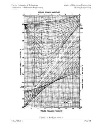
When gas is present in the well, the hydrostatic pressure developed by the gas column is calculated
with:
p = po.e
M.(D−Do)
1,544.z.(Tf +460) (4.2)
where:
z [1] ... real gas deviation factor
po [psi] ... surface pressure
D [ft] ... total depth (TVD)
Tf [F] ... bottom hole temperature of the formation
The molecular weight M of the gas is found as:
M =
80.3.z. (T + 460) .ρg
p
(4.3)
where:
ρg [ppg] ... density of the gas
T [F] ... average gas density
For practical purposes, the hydrostatics due to a complex fluid column are converted to an equiva-
lent single-fluid hydrostatic pressure. To do this, all individual hydrostatic pressures are summed
CHAPTER 4 Page 58](https://image.slidesharecdn.com/drillingengineering-160119095813/85/Drilling-engineering-66-320.jpg)
![Curtin University of Technology
Department of Petroleum Engineering
Master of Petroleum Engineering
Drilling Engineering
up for a specific depth pd and then converted to an equivalent mud weight ρe [ppg] that would
cause the same hydrostatic pressure.
ρe =
pd
0.052.D
(4.4)
Therefore the equivalent mud weight has to be always referenced to a specific depth.
As the mud is used to transport the cuttings from the bottom of the hole to the surface and
penetrated formations often contain a certain amount of formation gas, the mud column at the
annulus is usually mixed with solids and gas. This alters the weight of the mud at the annulus.
The new average mud weight ρm of a mixture containing mud and solids can be calculated as:
ρm =
n
i=1 mi
n
i=1 Vi
=
n
i+1 ρi.Vi
n
i=1 Vi
=
n
i=1
ρi.fi (4.5)
where:
mi [lbm] ... mass of component i
Vi [gal] ... volume of component i
ρi [ppg] ... density of component i
fi [1] ... volume fraction of component i
I should be noted that only solids that are suspended within the mud do alter the mud weight.
Settled particles do not affect the hydrostatic pressure.
If gas is present in the mud column as well, the density of the gas component is a function of the
depth and will decrease with decreasing pressure. In this way, the density of mud containing gas
is decreasing with decreasing depth.
When the gas-liquid mixture is highly pressured (e.g. deep section of the well), the variation of
the gas density can be ignored and the average mud density containing gas calculated with:
ρ = ρf .(1 − fg) + ρg.fg =
(ρf + M.Nν) .p
p + z.Nν.R.T
(4.6)
where:
fg =
z.Nν.R.T
p
1 + z.Nν.R.T
p
(4.7)
CHAPTER 4 Page 59](https://image.slidesharecdn.com/drillingengineering-160119095813/85/Drilling-engineering-67-320.jpg)
![Curtin University of Technology
Department of Petroleum Engineering
Master of Petroleum Engineering
Drilling Engineering
fg [1] ... volume fraction of gas
ρg [ppg] ... density of gas
Nν [# moles] ... moles of gas dispersed in one gallon of mud
When the variation of gas density can not be ignored (e.g. shallow depth), the equation 4.8 has
to be solved by iteration to compute the change in pressure:
D2 − D1 =
p2 − p1
0.052. (ρf + M.Nν)
+
z.Nν.R.T
0.052. (ρf + M.Nν)
. ln
p2
p1
(4.8)
where:
z is calculated at p = p2+p1
2
It is essential to understand that well control and the safety of drilling operations are strongly
depended on the maintenance of proper hydrostatic pressure. This pressure is needed to counter-
balance the formation pressure. In case the hydrostatic pressure in the borehole is higher than the
formation pressure, the situation is called “over-balanced”. This prevents kicks (fluid flow from the
formation into the borehole) and causes at permeable formations an intrusion of some mud (water
component) into the formation. The intrusion is stopped by the built up of mud cake that seals
off permeable formations. On the other hand, the hydrostatic pressure inside the borehole must
not be higher than the fracture pressure of the formations penetrated since this would fracture
the formation artificially, cause loss of circulation and lead to well control problems. To obtain
maximum penetration rates the hydrostatic pressure should be kept as close as practical to the
formation pressure since a higher differential pressure (hydrostatic pressure - formation pressure)
leads to worst cutting removal from the bottom of the well. Due to this circumstance, underbal-
anced drilling techniques have been developed that use air, foam or mist as drilling fluids. Here
the formation pressure is higher than the hydrostatic pressure caused by the mud and thus the
well is constantly kicking. With underbalanced drilling techniques much higher penetration rates
are possible but well control can be a problem. Therefore underbalanced drilling is prohibited by
some governments and/or in some areas.
4.2 Types of Fluid Flow
Since multiple aspects of drilling and completion operations require the understanding of how fluid
moves through pipes, fittings and annulus, the knowledge of basic fluid flow patterns is essential.
Generally, fluid movement can be described as laminar, turbulent or in transition between laminar
and turbulent.
It should be understood that rotation and vibrations influence the rheological properties of drilling
fluids. Also the pulsing of the mud pumps cause variations in the flow rates as well as the mean
flow rates. Furthermore changing solid content influences the actual mud density and its plastic
viscosity.
CHAPTER 4 Page 60](https://image.slidesharecdn.com/drillingengineering-160119095813/85/Drilling-engineering-68-320.jpg)
![Curtin University of Technology
Department of Petroleum Engineering
Master of Petroleum Engineering
Drilling Engineering
Fluid movement, when laminar flow is present, can be described as in layers or “laminae”. Here at
all times the direction of fluid particle movement is parallel to each other and along the direction
of flow. In this way no mixture or interchange of fluid particles from one layer to another takes
place. At turbulent flow behavior, which develops at higher average flow velocities, secondary
irregularities such as vortices and eddys are imposed to the flow. This causes a chaotic particle
movement and thus no orderly shear between fluid layers is present.
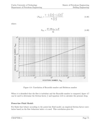
The so called “Reynolds number” is often used to distinguish the different flow patterns. Af-
ter defining the current flow pattern, different equations are applied to calculate the respective
pressure drops.
For the flow through pipes, the Reynolds number is determined with:
NRe =
928.ρm.ν.di
µ
(4.9)
ν =
q, [gal/min]
2.448.d2
i
=
17.16. (q, [bbl/min])
d2
i
(4.10)
and for the flow through annuli:
NRe =
928.ρm.ν.de
µ
(4.11)
ν =
q, [gal/min]
2.448. (d2
2 − d2
1)
=
17.16. (q, [bbl/min])
d2
2 − d2
1
(4.12)
de = 0.816. (d2 − d1) (4.13)
where:
ρ [ppg] ... fluid density
di [in] ... inside pipe diameter
ν [ft/sec] ... mean fluid velocity
µ [cp] ... fluid viscosity
de [in] ... equivalent diameter of annulus
d2 [in] ... internal diameter of outer pipe or borehole
d1 [in] ... external diameter of inner pipe
The different flow patterns are then characterised considering the Reynolds number. Normally
the Reynolds number 2,320 distinguishes the laminar and turbulent flow behavior, for drilling
purposes a value of 2,000 is applied instead. Furthermore it is assumed that turbulent flow is fully
CHAPTER 4 Page 62](https://image.slidesharecdn.com/drillingengineering-160119095813/85/Drilling-engineering-70-320.jpg)
![Curtin University of Technology
Department of Petroleum Engineering
Master of Petroleum Engineering
Drilling Engineering
developed at Reynolds numbers of 4,000 and above, thus the range of 2,000 to 4,000 is named
transition flow:
NRe < 2, 000 ... laminar flow
2, 000 < NRe < 4, 000 ... transition flow
NRe > 4, 000 ... turbulent flow
4.3 Rheological Classification of Fluids
All fluids encountered in drilling and production operations can be characterized as either “New-
tonian” fluids or “Non-Newtonian” ones. Newtonian fluids, like water, gases and thin oils (high
API gravity) show a direct proportional relationship between the shear stress τ and the shear rate
˙γ, assuming pressure and temperature are kept constant. They are mathematically defined by:
τ = µ.
−dνr
dr
= µ.˙γ (4.14)
where:
τ [dyne/cm2] ... shear stress
˙γ [1/sec] ... shear rate for laminar flow within circular pipe
µ [p] ... absolute viscosity [poise]
Figure 4.2: Newtonian flow model
A plot of τ vs. −dνr
dr
produces a straight line that
passes through the origin and has a slop of µ.
Most fluids encountered at drilling operations like
drilling muds, cement slurries, heavy oil and gelled
fracturing fluids do not show this direct relationship
between shear stress and shear rate. They are char-
acterized as Non-Newtonian fluids. To describe the
behavior of Non-Newtonian fluids, various models
like the “Bingham plastic fluid model”, the “Power-
law fluid model” and “Time-dependent fluid mod-
els” were developed where the Bingham and Power-
law models are called “Time-independent fluid
model” as well. The time dependence mentioned
here concerns the change of viscosity by the dura-
tion of shear. It is common to subdivide the time-
depended models into “Thixotropic fluid models”
and the“Rheopectic fluid models”.
CHAPTER 4 Page 63](https://image.slidesharecdn.com/drillingengineering-160119095813/85/Drilling-engineering-71-320.jpg)
![Curtin University of Technology
Department of Petroleum Engineering
Master of Petroleum Engineering
Drilling Engineering
Figure 4.3: Sketch of Bingham fluid model
It shall be understood that all the models men-
tioned above are based on different assumptions
that are hardly valid for all drilling operations, thus
they are valid to a certain extend only.
The Bingham and Power-law fluid models are de-
scribed mathematically by:
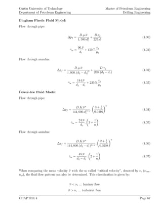
Bingham plastic fluid model:
τ = τy + µp
−dνr
dr
= τy + µp.˙γ (4.15)
Power-law fluid model:
τ = K.
−dνr
dr
n
= K.˙γn
(4.16)
Figure 4.4: Sketch of Power-law fluid model
where:
τy [lbf/100 ft2
] ... yield point
µp [cp] ... plastic viscosity
n [1] ... flow behavior index
K [1] ... consistency index.
A plot of shear stress vs. shear rate for the Bingham
model will result in a straight line, see sketch 4.3.
In contrary to Newtonian fluids, Bingham fluids do
have a yield point τy and it takes a defined shear
stress (τt) to initiate flow. Above τy, τ and γ are
proportional defined by the viscosity, re-named to
plastic viscosity µp
The characteristics of the Power-law fluid model is
sketched in 4.4. This plot is done on a log-log scale
and results in a straight line. Here the slope deter-
mines the flow behavior index n and the intercept
with the vertical, the value of the consistency index
(logK).
The flow behavior index, that ranges from 0 to
1.0 declares the degree of Non-Newtonian behav-
CHAPTER 4 Page 64](https://image.slidesharecdn.com/drillingengineering-160119095813/85/Drilling-engineering-72-320.jpg)
![Curtin University of Technology
Department of Petroleum Engineering
Master of Petroleum Engineering
Drilling Engineering
ior, where n = 1.0 indicates a Newtonian fluid. The consistency index K on the other hand gives
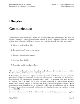
the thickness (viscosity) of the fluid where, the larger K, the thicker (more viscous) the fluid is.
Figure 4.5: Viscometer
To determine the rheological properties of a par-
ticular fluid, a rotational viscometer with six stan-
dard speeds and variable speed settings is used com-
monly. In field applications, out of these speeds just
two are normally used (300 and 600 [rpm]) since
they are sufficient to determine the required prop-
erties.
Following equations are applied to define the pa-
rameters of the individual fluid:
Newtonian fluid model:
µa =
300
N
.θN (4.17)
˙γ =
5.066
r2
.N (4.18)
Bingham plastic fluid model:
µp = θ600 − θ300 =
300
N2 − N1
. (θN2 − θN1 ) (4.19)
˙γ =
5.066
r2
.N +
479.τy
µp
.
3.174
r2
− 1 (4.20)
τy = θ300 − µp = θN1 − µp.
N1
300
(4.21)
τgel = θmax at N = 3 rpm (4.22)
Power-law fluid model:
n = 3.322. log
θ600
θ300
=
log
θN2
θN1
log N2
N1
(4.23)
CHAPTER 4 Page 65](https://image.slidesharecdn.com/drillingengineering-160119095813/85/Drilling-engineering-73-320.jpg)
![Curtin University of Technology
Department of Petroleum Engineering
Master of Petroleum Engineering
Drilling Engineering
K =
510.θ300
511n
=
510.θN
(1.703.N)n
(4.24)
˙γ = 0.2094.N.
1
r
2
n
n. 1
r
2
n
1
− 1
r
2
n
2
(4.25)
where:
r2 [in] ... rotor radius
r1 [in] ... bob radius
r [in] ... any radius between r1 and r2
θN [1] ... dial reading of the viscometer at speed N
N [rpm] ... speed of rotation of the outer cylinder
4.4 Laminar Flow in Pipes and Annuli
For drilling operations the fluid flow of mud and cement slurries are most important.
When laminar flowing pattern occurs, the following set of equations can be applied to calculate
the friction pressure drop [psi], the shear rate at the pipe wall and the circulation bottom hole
pressure for the different flow models:
Newtonian Fluid model:
Flow through pipe:
∆pf =
D.µ.ν
1, 500.d2
i
(4.26)
˙γw =
96.ν
di
(4.27)
Flow through annulus:
∆pf =
D.µ.ν
1, 000. (d2 − d1)2 (4.28)
˙γw =
144.ν
d2 − d1
(4.29)
CHAPTER 4 Page 66](https://image.slidesharecdn.com/drillingengineering-160119095813/85/Drilling-engineering-74-320.jpg)
![Curtin University of Technology
Department of Petroleum Engineering
Master of Petroleum Engineering
Drilling Engineering
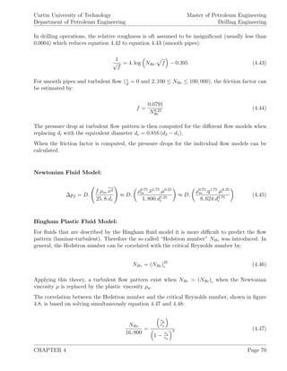
The critical velocities are calculated for the different models as:
Bingham Plastic Fluid Model:
Flow through pipe, νcp in [ft/sec]:
νcp =
1.078.µp + 1.078. µ2
p + 12.34.ρm.d2
i .τy
ρm.di
(4.38)
Flow through annulus, νcan in [ft/sec]:
νcan =
1.078.µp + 1.078. µ2
p + 9.256.ρm. (d2 − d1)2
.τy
ρm. (d2 − d1)
(4.39)
Power-law Fluid Model:
Flow through pipe, νcp in [ft/min]:
νcp =
5.82.104
.K
ρm
1
2−n
.
1.6
di
.(
3.n + 1
4.n
)
n
2−n
(4.40)
Flow through annulus, νcan in [ft/min]:
νcan =
3.878.104
.K
ρm
1
2−n
.
2.4
d2 − d1
.(
2.n + 1
3.n
)
n
2−n
(4.41)
4.5 Turbulent Flow in Pipes and Annuli
To describe the flow behaviour, friction pressure loss and shear rate at the pipe wall for laminar
flow, analytic equations are applied. For turbulent fluid flow behavior, analytic models to calculate
these parameters are extremely difficult to derive. Therefore, various concepts that describe their
behavior are used in the industry.
The concept based on the dimensionless quantity called “Friction factor” is the most widely applied
correlation technique. Following equation can be used to determine the friction factor for fully
developed turbulent flow pattern:
1
√
f
= −4. log 0.269.
d
+
1.255
NRe.
√
f
(4.42)
where:
CHAPTER 4 Page 68](https://image.slidesharecdn.com/drillingengineering-160119095813/85/Drilling-engineering-76-320.jpg)
![Curtin University of Technology
Department of Petroleum Engineering
Master of Petroleum Engineering
Drilling Engineering
[in] ... absolute roughness of pipe, see table 4.6
d
[1] ... relative roughness of pipe
Figure 4.6: Absolute pipe roughness for several types of circular pipes
To solve this equation for f, iteration techniques have to be applied . The friction factor can also
be obtained from figure 4.7.
Figure 4.7: Friction factor for turbulent flow
CHAPTER 4 Page 69](https://image.slidesharecdn.com/drillingengineering-160119095813/85/Drilling-engineering-77-320.jpg)
![Curtin University of Technology
Department of Petroleum Engineering
Master of Petroleum Engineering
Drilling Engineering
Flow through pipe:
µa =
K.d1−n
i
96.ν1−n .
3 + 1
n
0.0416
n
(4.50)
NRe =
89, 100.ρm.ν2−n
K
.
0.0416.di
3 + 1
n
n
(4.51)
Flow through annulus:
µa =
K. (d2 − d1)1−n
144.ν1−n .
2 + 1
n
0.0208
n
(4.52)
NRe =
109, 000.ρm.ν2−n
K
.
0.0208. (d2 − d1)
2 + 1
n
n
(4.53)
where:
µa [cp] ... apparent Newtonian viscosity
NRe > (NRe)c ... turbulent flow
This Reynolds number is then compared with the critical Reynolds number, which is depended
on the flow behaviour index n and should be obtained from figure 4.9 as a starting point of the
turbulent flow line for the given n, resulting in:
Instead of using figure 4.9, equation 4.54 can be applied to determine the friction factor iteratively:
1
f
=
4.0
n0.75
. log NRe.f1− n
2 −
0.395
n1.2
(4.54)
When the friction factor f is calculated, the corresponding pressure drop can be calculated with
equation 4.45.
CHAPTER 4 Page 72](https://image.slidesharecdn.com/drillingengineering-160119095813/85/Drilling-engineering-80-320.jpg)
![Curtin University of Technology
Department of Petroleum Engineering
Master of Petroleum Engineering
Drilling Engineering
Figure 4.9: Friction factor for Power-Law fluid model
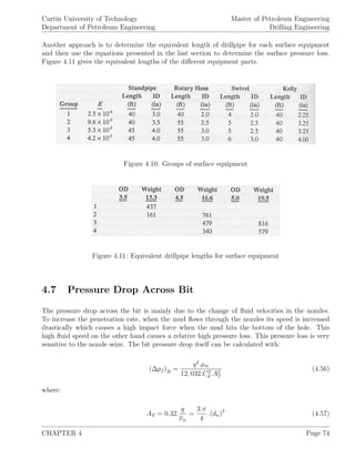
4.6 Pressure Drop Across Surface Connections
The pressure drop in surface connections comprise the pressure drops along the standpipe, the
rotary hose, swivel and kelly. Since different rigs do use different equipment, the total pressure
loss at the surface equipment can only be estimated. This is performed with equation 4.55:
(∆pf )se = E.ρ0.8
m .q1.8
.µ0.2
p (4.55)
where:
(∆pf )se [psi] ... pressure loss through total surface equipment
q [gpm] ... flow rate
E [1] ... constant depending on the type of surface equipment
used, see figure 4.10
CHAPTER 4 Page 73](https://image.slidesharecdn.com/drillingengineering-160119095813/85/Drilling-engineering-81-320.jpg)
![Curtin University of Technology
Department of Petroleum Engineering
Master of Petroleum Engineering
Drilling Engineering
νn = Cd
1, 238. (∆pf )B
ρm
(4.58)
dn = 32.
4.AT
3.π
(4.59)
AT [in2
] ... total nozzle area
dn [1/32] ... jet nozzle seize
νn [ft/sec] ... mean nozzle velocity
q [gpm] ... flow rate
ρm [ppg] ... mud density
Cd [1] ... discharge coefficient, depending on the nozzle type and
size (commonly Cd = 0.95)
4.8 Initiating Circulation
All the equations to calculate the individual pressure drops presented above assume a non-
thixotropic behavior of the mud. In reality, an additional pressure drop is observed when cir-
culation is started due to the thixotropic structures which have to be broken down. This initial
phase of addition pressure drop may last for one full circulation cycle. The additional pressure
drop can be estimated applying the gel strength τg of the drilling mud as:
For flow through pipes:
(∆pf )p = D.
τg
300.di
(4.60)
For flow through annuli:
(∆pf )an = D
τg
300. (d2 − d1)
(4.61)
where:
τg [lbf/100 ft2
] ... gel strength of the drilling mud
CHAPTER 4 Page 75](https://image.slidesharecdn.com/drillingengineering-160119095813/85/Drilling-engineering-83-320.jpg)

![Curtin University of Technology
Department of Petroleum Engineering
Master of Petroleum Engineering
Drilling Engineering
The pressure drop across the bit can be written as:
Hydraulic horsepower:
(∆pf )B−opt = pmax − (∆pf )d−opt = pmax −
1
1 + m
.pmax (4.64)
Jet impact force:
(∆pf )B−opt = pmax − (∆pf )d−opt = pmax −
2
2 + m
.pmax (4.65)
where:
m [1] ... slope of the parasitic pressure loss (∆pf )d vs. flow rate
Theoretically m = 1.75 but in general it is better to determine m from field data than assuming
this value.
When plotting flow rate vs. pressure on a log-log plot, the optimum design is found at the
intersection between the path of optimum hydraulics and the (∆pf )d line for either of the criteria
mentioned above.
Having determined the optimum design, the optimum pump flow rate, optimum nozzle area and
corresponding pressure losses can be calculated:
(AT )opt =
(qopt)2
.ρm
12, 032.C2
d . (∆pf )B−opt
(4.66)
(dn)opt = 32.
4. (AT )opt
3.π
(4.67)
Optimum hydraulic horsepower and jet impact force are given with:
(hp)opt =
(∆pf )B−opt .qopt
1, 714
(4.68)
(Fj)opt = 0.01823.Cd.qopt. ρm. (∆pf )B−opt (4.69)
The optimum nozzle area leads to the respective nozzle selection. Nozzles for drilling bits are given
1
32
[in] seizes thus the calculated nozzle area has to be converted into n
32
[in]. Knowing n (has to
CHAPTER 4 Page 77](https://image.slidesharecdn.com/drillingengineering-160119095813/85/Drilling-engineering-85-320.jpg)
![Curtin University of Technology
Department of Petroleum Engineering
Master of Petroleum Engineering
Drilling Engineering
be an integer and is commonly rounded down to ensure the nozzle velocity) and the amount of
nozzles to use, the individual seizes are found.
The so called “specific hydraulic horsepower” is defined as hydraulic horsepower per unit borehole
cross-section.
(hp)spec
=
4.hp
π.d2
BH
(4.70)
The optimization as discussed above is performed for regular intervals (e.g. 1,000 [ft]) and is
included in the drilling program. In practice, computer programs are available in the industry
that perform these hydraulic optimization calculations.
4.10 Particle Slip Velocity
The annular flow of the drilling fluid carrying drilling cuttings and a certain amount of gas to the
surface, is disturbed by frictional and centrifugal forces caused by the rotation of the drillstring.
In practice, when it is noticed that inefficient hole cleaning is present, either the mud flow rate is
increased or the effective viscosity of the mud is increased or both adjustments are performed.
To estimate the slip velocity of the cuttings, following correlation methods were developed empir-
ically and are widely accepted and used in the industry:
Moore’s Correlation:
µa =
K
144
.
d2 − d1
νan
1−n
.
2 + 1
n
0.0208
n
(4.71)
for NRp > 300:
νsl = 1.54. ds.
ρs − ρm
ρm
(4.72)
for NRp < 3:
νsl = 82.87.
d2
s
µa
. (ρs − ρm) (4.73)
for 3 ≤ NRp < 300:
νsl =
2.90.ds. (ρs − ρm)0.667
ρ0.333
m .µ0.333
a
(4.74)
CHAPTER 4 Page 78](https://image.slidesharecdn.com/drillingengineering-160119095813/85/Drilling-engineering-86-320.jpg)
![Curtin University of Technology
Department of Petroleum Engineering
Master of Petroleum Engineering
Drilling Engineering
where:
NRp =
928.ρm.νsl.ds
µa
(4.75)
ds =
τg
10.4. (ρs − ρm)
(4.76)
µa [cp] ... apparent Newtonian viscosity
ds [in] ... drilling cuttings diameter
NRp [1] ... particle Reynolds number
νsl [ft/sec] ... particle slip velocity
ρs [ppg] ... cuttings density
τg [lbf/100 ft2
] ... gel strength required to suspend a particle of diameter ds
Chien’s Correlation:
The correlation equations determined by Chien are similar to the ones defined by Moore. For
clay-water muds, he recommends the usage of the apparent viscosity.
µa = µp + 5.
τy.ds
νa
(4.77)
The correlation is performed as:
for NRp < 100:
νsl = 0.0075.
µa
ρm.ds
.
36, 800.ds
µa
ρm.ds
2 .
ρs − ρm
ρm
+ 1 − 1
(4.78)
for NRp > 100:
νsl = 1.44.
d2
s
µa
(ρs − ρm) (4.79)
The so called “transportation velocity” νT is defined as the difference between the mean annular
velocity νan and the slip velocity νsl. The “transportation ratio” FT given by:
FT =
νT
νan
(4.80)
CHAPTER 4 Page 79](https://image.slidesharecdn.com/drillingengineering-160119095813/85/Drilling-engineering-87-320.jpg)
![Curtin University of Technology
Department of Petroleum Engineering
Master of Petroleum Engineering
Drilling Engineering
determines whether the cuttings are transported to the surface (FT is positive) or not and provides
a relative measure of the carrying capability of the drilling mud.
To have proper hole cleaning and with the knowledge of the transport velocity, a minimum mean
annular velocity can be determined. This minimum mean annular velocity has to be calculated at
the annulus with the maximum cross-section area and in this way determines the minimum pump
rate. As a rule of thumb, a minimum mean annular velocity of 3 [ft/sec] is often applied.
4.11 Surge and Swab Pressure
When running tubulars in a hole filled with drilling mud so called “surge pressures” and “swab
pressures” are created. The surge pressure is an increase of the pressure in front of the tubulars
when run into the well, the swab pressure is a pressure reduction behind the tubular when pulled
out of the well. Excessive surge or swab pressures have to be avoided since they can lead to
problems like:
1. Pressure reduction due to swab can cause a kick,
2. Pressure increase due to surge pressure can fracture weaker formation and cause lost circu-
lation which in turn can cause a kick,
3. Swab pressure increases the intake of formation gas (trip gas) which in turn can decrease
the hydrostatic pressure.
The parameters that determine surge and swab pressures are: mud rheological properties, tubular
velocity, tubular and hole geometry. The mean annular fluid velocity caused by tubular movement
is by definition positive when moved upward and negative when moved downward. It is calculated
for:
closed tubulars:
νan−closed = νp. 0.45 +
d2
p
d2
h − d2
p
(4.81)
open tubulars:
νan−open = νp. 0.45 +
d2
p − d2
i
d2
h − d2
p + d2
i
(4.82)
νmax = 1.5.νan (4.83)
The corresponding pressure drop is calculated assuming the power-law model and the correspond-
ing factors n and K:
CHAPTER 4 Page 80](https://image.slidesharecdn.com/drillingengineering-160119095813/85/Drilling-engineering-88-320.jpg)
![Curtin University of Technology
Department of Petroleum Engineering
Master of Petroleum Engineering
Drilling Engineering
(∆pf ) =
2.4.νmax
dh − dp
.
2.n + 1
3.n
n
.
K.D
300. (dh − dp)
(4.84)
where:
νp [ft/min] ... tubular velocities
dh [in] ... diameter of the borehole
dp [in] ... outer diameter of the drillpipe or drill collar
di [in] ... inner diameter of the drillpipe or drill collar
D [ft] ... total pipe length
CHAPTER 4 Page 81](https://image.slidesharecdn.com/drillingengineering-160119095813/85/Drilling-engineering-89-320.jpg)
![Curtin University of Technology
Department of Petroleum Engineering
Master of Petroleum Engineering
Drilling Engineering
4.12 Examples
1. To cement a casing string at a depth of 8,500 [ft] the used 10 [ppg] drilling mud is to be
displaced from the annulus by a 600 [ft] preflush of 9 [ppg] mud, 1,800 [ft] of 12.5 [ppg] filler
cement and 1,600 [ft] of 16.0 [ppg] high-strength cement. After the high-strength cement, brine
with 8.5 [ppg] is pumped as spacer. Compute the:
(a) Minimum pump pressure required to completely
displace the casing,
(b) Equivalent mud weight at 8,500 [ft] after the cement
has been displaced completely from the casing.
2. A non-Newtonian fluid is measured by a rotation viscosimeter giving readings of 22 at 300
[rpm] and 39 at 600 [rpm] respectively. When the fluid is characterised by the Bingham plastic
fluid model, µp and τy is to be determined, when the power-law model is applied, the consistency
and flow behavior index have to be computed.
3. A fluid characterized by the Bingham plastic fluid model has a yield point of 12 [lbf/ 100 ft]
and a plastic viscosity of 50 [cp]. When the flow pattern is laminar, the pressure drop due to
friction at 8,000 [ft] is to be computed for a:
(a) flow rate of 50 [gpm] through a drillstring
with 3.826 [in] ID,
(b) flow rate of 90 [gpm] through a 10 X 7 [in]
annulus.
4. When drilling a well to 1,000 [ft], a Bingham plastic fluid with a yield point of 5 [lbf/ 100 ft]
and plastic viscosity of 25 [cp] is applied. Using following additional information (Ldp = 1, 000
[ft], di = 3.826 [in], d1 = 4.5 [in], d2 = 6.5 [in], q = 500 [gpm], d
= 0) calculate the:
(a) Flow pattern in the drillpipe,
(b) Flow pattern in the annulus opposite the drillpipe,
(c) Frictional pressure loss in the drillpipe,
(d) Frictional pressure loss in the annulus.
5. Assuming the same mean flow velocities and a power-law fluid model with a consistency index
of 200 [eq cp] and flow behavior index of 0.75, calculate the same values at in example 4.
CHAPTER 4 Page 82](https://image.slidesharecdn.com/drillingengineering-160119095813/85/Drilling-engineering-90-320.jpg)
![Curtin University of Technology
Department of Petroleum Engineering
Master of Petroleum Engineering
Drilling Engineering
6. A jet bit shall produce a 800 [psi] pressure drop through the nozzles when circulating 900 [gpm]
of 10 [ppg] drilling mud. Select 3 nozzles that produce this pressure drop and calculate the jet
velocity of the mud.
7. A 11.75 [in] casing with a closed end is lowered into a 12.25 [in] hole at a rate of 1.5 [ft/sec].
What is the equivalent density below the bottom joint at 7,000 [ft] when the hole is filled with a
10.5 [ppg] mud having a viscosity of 2.5 [cp]?
8. When drilling with a 10 [ppg] mud and a bit, using three 12
32
[in] nozzles, the pump pressure
at a flow rate of 500 [gpm] is 3,000 [psi]. When the frow rate is dropped to 250 [gpm], a pump
pressure of 800 [psi] is recorded. The minimum flow rate to lift the cuttings is determined as 240
[gpm], the maximum allowable surface pressure is 3,000 [psi]. The pump itself is rated at 1,000
[hp] and exhibits an overall efficiency of 90 %. Compute the:
(a) Proper operating conditions and bit nozzle sizes for
maximum bit horsepower for the next bit run¿,
(b) Bit horsepower required to obtain the conditions selected,
(c) Jet impact force obtained at the conditions selected,
(d) Jet nozzle velocity obtained at the conditions selected.
CHAPTER 4 Page 83](https://image.slidesharecdn.com/drillingengineering-160119095813/85/Drilling-engineering-91-320.jpg)

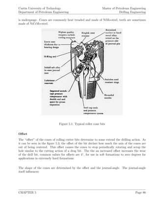
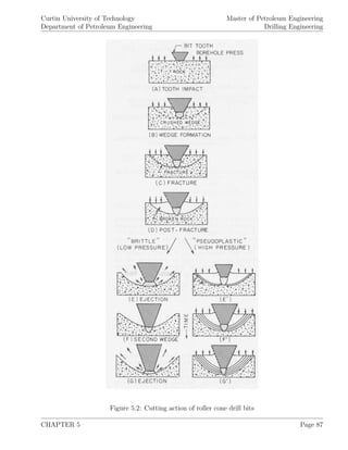
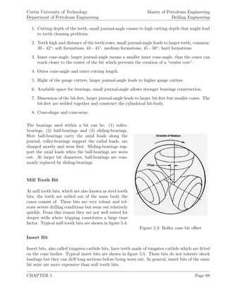
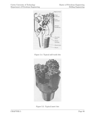
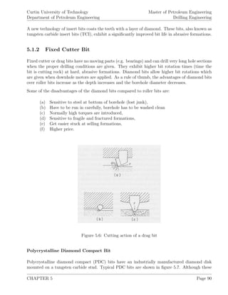
![Curtin University of Technology
Department of Petroleum Engineering
Master of Petroleum Engineering
Drilling Engineering
bits are very expensive, under the propper drilling conditions, they can drill very fast for long
distances. Thus they are most often applied for offshore drilling (high rig rates) and deep wells
(tripping time).
Figure 5.7: Typical PDC bits
The PDC bit itself consists of a steel
body where the tungsten carbide studs
are mounted on steel pegs which are fit
into holes of the body. Bits that are con-
structed from molded tungsten carbide
are also called “matrix body bits”. Ma-
trix body bits are more expensive than
PDC bits but they exhibit less wear (e.g
loss of teeth in hole).
PDC bits are manufactured in many
different shapes that determine their
behavior to rather drill directional or
straight trajectories. The different
shapes of the PDC bits also govern
the amount, profile and seize of cutters
mounted on the surface.
Polycrystalline Diamond Bit
Polycrystalline diamond (PCD) bits consist of industrially manufactured, temperature stable di-
amonds that are mounted directly into the bit matrix.
Natural Diamond Bit
Natural diamond bits wear out the rock at the bottom of the hole by producing very small cuttings
known as “rock flour”. Typical natural diamond bits are shown in figure 5.8. These bits can drill
the hardest rocks (highest compressive strength) but they drill relatively slowly and are very
expensive. For this reason they are used at very hard and very abrasive formations which would
destroy other types of bits before making reasonable drilling progress. Diamonds used for these
bits are naturally occurring industrial-grade ones. The diamonds are mounted with an exposure
of 1/100 to 1/1000 [mm], having diamond seizes of 1 to 100 [St/ct]. Impregnated diamond bits
have diamond-splints (seize > 100 [St/ct]) mixed into their matrix-body. Thus when the bit wears
out (body wears), new diamonds-splints out of the body become exposed and the bit stays sharp.
Fishtail Bit
This type of bit was developed at the early days of oil well drilling and look, when viewed from
the side, somewhat like a fishtail. They are only applicable at soft formations where they establish
CHAPTER 5 Page 91](https://image.slidesharecdn.com/drillingengineering-160119095813/85/Drilling-engineering-99-320.jpg)
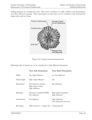
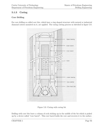
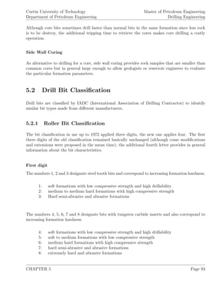
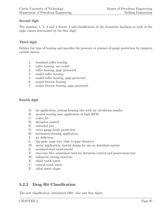
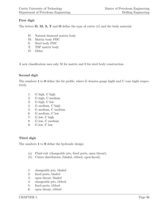
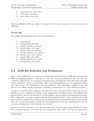
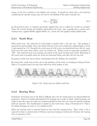
![Curtin University of Technology
Department of Petroleum Engineering
Master of Petroleum Engineering
Drilling Engineering
5.3.3 Gauge Wear
When the gauge teeth of a bit are worn, the drilled hole will be under-gauge with may lead to
damage of the next bit. Measurement of the gauge wear is performed with the help of a ringe
gauge and a ruler. The loss of diameter in [in] is reported as the nearest eighth, denoting with the
letter O for “out of gauge”. In this way, a bit which diameter is reduced by 0.5 [in] is reported as
G-O-4 (4 since 4
8
[in]). When the bit is in-gauge, it is reported using the letter I.
In addition to the wear gradings listed above, the bit record commonly includes a column of
comments. Here the bit conditions are commonly remarked.
5.4 Factors that Affect the Rate Of Penetration
Although through out the text, various aspects that influence the ROP are mentioned when
appropriate, the following considerations are often applied to determine the drilling parameters
recommended.
5.4.1 Bit Type
The type of bit applied to drill a certain formation has a large impact on the achieved penetration
rate. Roller cutting bits with long teeth exhibit commonly the highest penetration rates but they
are only applicable at soft formations. At hard formations where drag bits dominate, the realised
ROP is mainly a function of seize and amount of cutters along with an optimum combination of
drilling parameters.
5.4.2 Formation Characteristics
The most important formation properties that determine the penetration rate are the elastic limit
and the ultimate rock strength. To estimate the strength of a formation, the shear strength by
the Mohr failure criteria is often used.
When drilling is initiated, a threshold force or bit weight W
d t
has to be overcome. This threshold
force can be found when plotting drilling rates as a function of bit weight per diameter and then
extrapolated back to zero drilling rate.
Another formation property that has a large influence to the realized ROP is its permeability. At
rocks with high permeability, the drilling mud is forces into the rock ahead of the bottom of the
hole and thus reduces the differential pressure.
Other rock properties like its abrasiveness and gummy clay minerals content contribute indirectly
to the ROP by influencing the drilling bit (wear, dulling, etc.).
CHAPTER 5 Page 99](https://image.slidesharecdn.com/drillingengineering-160119095813/85/Drilling-engineering-107-320.jpg)
![Curtin University of Technology
Department of Petroleum Engineering
Master of Petroleum Engineering
Drilling Engineering
Figure 5.11: Threshold force to initiate drilling in different formations
5.4.3 Drilling Fluid Properties
From the various drilling fluid properties, following were identified as influencing the penetration
rate:
(a) drilling fluid density,
(b) rheological flow properties,
(c) filtration characteristics,
(d) solids content and distribution,
(e) chemical composition.
It was found that penetration rate decreases with increasing fluid density, viscosity and solids
content and increases with increasing filtration rate. This is mainly caused by influencing the
differential pressure at the bottom of the hole. The drilling fluid viscosity on the other hand
controls the pressure losses along the drillstring and thus the available hydraulic impact force at
the bit. It has also been found that the content of solids particles with a seize less than 1 [µm]
(colloid seize) do influence the ROP dramatically since they are plugging of filtration below the
bit.
As it can be seen in figure 5.13, the penetration rate is largely dependent on the differential
pressure. It should be noted that a change in differential pressure when it is low causes a large
CHAPTER 5 Page 100](https://image.slidesharecdn.com/drillingengineering-160119095813/85/Drilling-engineering-108-320.jpg)
![Curtin University of Technology
Department of Petroleum Engineering
Master of Petroleum Engineering
Drilling Engineering
Figure 5.12: Variation of penetration rate with different mud properties
change in ROP, when the differential pressure is high, a change of it influences the penetration
rate only slightly.
The effective differential pressure at the bottom of the hole does not only have an influence to
the cutting action, it also influences the chip removal and therefore the cleaning of the bottom
hole. When plotting a ROP relation on a semilog scale, a straight line can be interpolated that
estimates the penetration rate for various overbalances, see figure 5.14.
Figure 5.14 can be described with equation 5.2:
log
R
R0
= −m.(pbh − pf ) (5.2)
where:
R [ft/hr] ... penetration rate with particular overbalance
R0 [ft/hr] ... penetration rate with zero overbalance
m [1] ... slope of the correlation line
pbh [psi] ... bottom hole pressure in the borehole
pf [psi] ... formation fluid pressure
CHAPTER 5 Page 101](https://image.slidesharecdn.com/drillingengineering-160119095813/85/Drilling-engineering-109-320.jpg)
![Curtin University of Technology
Department of Petroleum Engineering
Master of Petroleum Engineering
Drilling Engineering
Figure 5.13: Effect of overbalance on drilling rate in Indiana limestone for clay/water mud and
1.25 [in] roller cutting bit
Figure 5.14: Exponential relationship between penetration rate and overbalance for roller cutting
bits
When the overbalance is expressed with the equivalent circulation mud density ρc and the pore
pressure gradient gp (both [ppg]) using equation 5.3, and the factor 0.052.m as a4, the change of
penetration rate can be estimated due to the change of mud weight by applying equation 5.4.
CHAPTER 5 Page 102](https://image.slidesharecdn.com/drillingengineering-160119095813/85/Drilling-engineering-110-320.jpg)
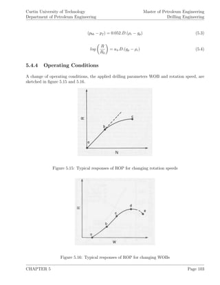


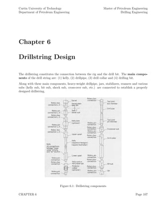
![Curtin University of Technology
Department of Petroleum Engineering
Master of Petroleum Engineering
Drilling Engineering
Some problems that can arise due to improper design of the drillstring are twistoffs, collapse
failures or washouts.
In general, the drillstring provides multiple functions like:
1. Imposes required weight on the bit
2. Transmits rotary motion from the kelly to the drill bit
3. Provides a two way fluid conduit from the rig to the drill bit
4. Medium to lower and raise the drill bit in the hole
5. Stabilizes the bottom hole assembly (BHA) and minimizes vibrations
6. Permits pressure and formation fluid testing through the drillstring
7. Allows through-pipe running of formation evaluation tools when they can not be run in the
open hole
The following sections discusses various design criteria like determination of appropriate length
and grade of drill pipe as well as drill collars, placement of stabilizers and reamers, dogleg severity
analysis and calculation of critical rotary speeds.
6.1 Drill Pipe Classification
Grades of drillpipe
API steel grades for drill pipe:
Steel grade Min.Yield [psi] Max.Yield [psi] Min.Tensil [psi]
E75 75,000 105,000 100,000
X95 95,000 125,000 105,000
G105 105,000 135,000 115,000
S135 135,000 165,000 145,000
Non-API special H2S Steel for drill pipes:
Steel grade Min.Yield [psi] Max.Yield [psi] Min.Tensil [psi]
DP-80 VH 80,000 95,000 95,000
DP-95 VH 95,000 110,000 105,000
MW-CE-75 75,000 90,000 95,000
MW-CX-95 95,000 110,000 105,000
CHAPTER 6 Page 108](https://image.slidesharecdn.com/drillingengineering-160119095813/85/Drilling-engineering-116-320.jpg)
![Curtin University of Technology
Department of Petroleum Engineering
Master of Petroleum Engineering
Drilling Engineering
Common diameters of drillpipe are: 2-3/8, 2-7/8, 3-1/2, 4, 4-1/2, 5, 5-1/2, 6-5/8 [in], where the
5 [in] drillpipe is the most often used one.
The length of one drillpipe is according to APT ranges:
Range 1 18 to 22 [ft]
Range 2 27 to 30 [ft]
Range 3 38 to 45 [ft]
All size, weights and grades are classified according to their use as:
Class I white band new pipe, everything nominal
Premium class two white bands reductions generally up to 80%
Class II yellow band reductions generally up to 70%
Class III orange band any imperfections or damages exceeding class II
The different classes are also used to reduce the nominal yield strength where following wear
assumptions are made:
Premium wear rate: 20%,
Class II wear rate: 20%,
Class III wear rate: 37.5%,
The end of drillpipes can be manufactured geometrically different. The female portion of the tool
joint is called “box”, the male portion “pin”. The portion of the drillpipe to which the tool joint
is attached has a larger wall-thickness than the rest of the drillpipe and is called “upset”. The
upset can be shaped as: internal upset (IU), external upset (EU) and internal and external upset
(IEU), see figure 6.2.
Figure 6.2: Geometric ending of drillpipe
CHAPTER 6 Page 109](https://image.slidesharecdn.com/drillingengineering-160119095813/85/Drilling-engineering-117-320.jpg)
![Curtin University of Technology
Department of Petroleum Engineering
Master of Petroleum Engineering
Drilling Engineering
Tool joints are manufactures as regular, full hole and internal flush.
So called heavy weight drillpipe or heavy wall drillpipe are often applied in between drillpipe
and drill collars. They are manufactured with outside diameters ranging from 3-1/2 [in] to 5 [in]
and are used to reduce the sharp change of cross-area and stiffness from drillpipe to drill collars
which otherwise leads to fatigue failure.
6.2 Calculation of Neutral Point
Figure 6.3: Sketch of buckling tendency of drillstring
When the drillstring is low-
ered into the borehole, the total
length of the drillstring is under
tension due to its own weight
which is partly counterbalanced
by the buoyancy. To drill a well,
the rock beneath the bit has to
be destroyed. Part of this de-
struction force is obtained by
a certain amount of weight on
bit (WOB) which forces the bit
against the rock. Therefore
during drilling, the lower part
of the drill string is set under
compression, leaving the upper
part of it still under tension.
According to Lubinski, the neu-
tral point is defined as point
along the drillstring where it is
divided into two parts, an up-
per part, being suspended from
the elevators and which is un-
der tension as well as a lower
part that generates the appro-
priate WOB and is under com-
pression.
Due to the geometrical shape of
the drillstring (length/diameter
ratio), it has a tendency to
buckle. To reduce this buckling
tendency, it is aimed to design
the drillstring in such a way
that the neutral point is located
inside drilling collars. This de-
CHAPTER 6 Page 110](https://image.slidesharecdn.com/drillingengineering-160119095813/85/Drilling-engineering-118-320.jpg)
![Curtin University of Technology
Department of Petroleum Engineering
Master of Petroleum Engineering
Drilling Engineering
sign criteria is often used to evaluate the length of required collars. Taking these considerations
into account, the neutral point can be calculated for different scenarios as:
In the absence of mud (drilling with air as drilling fluid):
ln =
WOB
12.Ws
(6.1)
In the presence of drilling mud:
ln =
WOB
12. (Ws − ρs.As)
(6.2)
When differential pressure is considered as well, the neutral point is found at:
ln =
WOB
12. (Ws − ρe.Ae + ρi.Ai)
(6.3)
where:
ln [ft] ... distance of neutral point from the bottom of the hole
WOB [lbm] ... weight on bit applied
Ws [lbm/in] ... average weight in air of the tube per unit length
ρs [lbm/in3
] ... density of tubing
As [in2
] ... cross-sectional area of the tubing wall
ρe [lbm/in3
] ... density of mud in the annulus
Ae [in2
] ... area corresponding to tubing OD
ρi [lbm/in3
] ... density of mud in the tubing
Ai [in2
] ... area corresponding to tubing ID
6.3 Drillstring Design Calculations
As mentioned above, to prevent the drillstring from buckling, the neutral point must be placed
inside the drilling collars.
Other influencing factors for the drillstring design are: depth and seize of the well, applied mud
weights, desired safety factors, minimum margin of overpull, desired drillpipe seize and class as
well as applied WOB. The design itself is based on meeting tension, collapse, shock loading and
torsion requirements.
CHAPTER 6 Page 111](https://image.slidesharecdn.com/drillingengineering-160119095813/85/Drilling-engineering-119-320.jpg)
![Curtin University of Technology
Department of Petroleum Engineering
Master of Petroleum Engineering
Drilling Engineering
6.3.1 Tension
The total weight when the drillstring is suspended into the borehole is carried by the top joint of
the string. This weight [lb] is given by:
P = (Ldp.Wdp + Lhw.Whw + Ldc.Wdc) .BF (6.4)
where:
L [ft] ... total length of the individual tubular
W [lb/ft] ... nominal weight of the individual tubular
BF [1] ... buoyancy factor
Figure 6.4: Table of drillpipe properties
CHAPTER 6 Page 112](https://image.slidesharecdn.com/drillingengineering-160119095813/85/Drilling-engineering-120-320.jpg)
![Curtin University of Technology
Department of Petroleum Engineering
Master of Petroleum Engineering
Drilling Engineering
with the indices dp for drillpipe, hw for heavy-weight drillpipe and dc for drill collar.
The buoyancy factor BF, assuming that the drillstring is not lowered empty (ρsteel = 65.5 [ppg]),
can be computed as:
BF = 1 −
ρmud
ρsteel
(6.5)
Figure 6.5: Table of drillpipe properties con.
Ordinary, a safety factor of 0.9 is applied to calculate the maximum allowed yield strength Pa
from the drillpipe yield strength Pt, which is taken from tables 6.4 through 6.9:
Pa = 0.9.Pt (6.6)
CHAPTER 6 Page 113](https://image.slidesharecdn.com/drillingengineering-160119095813/85/Drilling-engineering-121-320.jpg)
![Curtin University of Technology
Department of Petroleum Engineering
Master of Petroleum Engineering
Drilling Engineering
or when the class wear rate is applied:
Pa = Pt.(1 − wear rate) (6.7)
Figure 6.6: Table of drillpipe properties con.
Having the maximum allowed yield strength and the total weight carried, the so called margin of
overpull (MOP) is defined by the difference of them:
MOP = Pa − P (6.8)
Knowing the MOP is important in case of stuck pipe when an additional pulling force has to
be applied to free the drillstring. In practice, the determined margin of overpull must not be
exceeded since the drillpipe would fail otherwise. Typical values of MOPs requirements for drillpipe
selections are in the range from 50,000 to 100,000 [lbf].
CHAPTER 6 Page 114](https://image.slidesharecdn.com/drillingengineering-160119095813/85/Drilling-engineering-122-320.jpg)
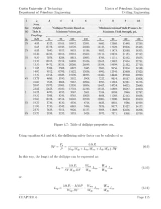
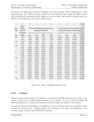
![Curtin University of Technology
Department of Petroleum Engineering
Master of Petroleum Engineering
Drilling Engineering
Figure 6.9: Table of drillpipe properties con.
The resulting differential pressure can be calculated prior to opening the DST tool, knowing the
length of the fluid inside the drillstring Y [ft], a total length of the drillstring L [ft] and the
densities ρ1 [ppg] of the fluid outside the drillpipe and ρ2 [ppg] of the fluid inside drillpipe. Note
that both Y and L are in TVD.
∆p =
L.ρ1
19.251
−
(L − Y ) .ρ2
19.251
(6.12)
When the drillpipe is completely empty (ρ2
∼= 0) the differential pressure is found to be:
∆p =
L.ρ1
19.251
(6.13)
When the fluids inside and outside the drillpipe are the same(ρ1 = ρ2 = ρ), the differential pressure
is:
CHAPTER 6 Page 117](https://image.slidesharecdn.com/drillingengineering-160119095813/85/Drilling-engineering-125-320.jpg)
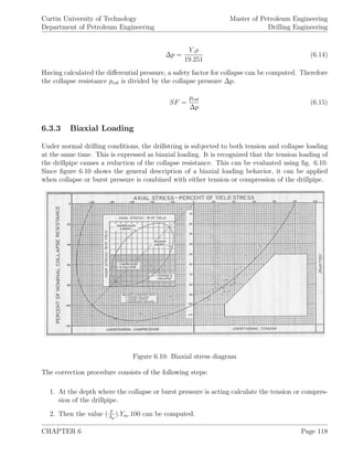
![Curtin University of Technology
Department of Petroleum Engineering
Master of Petroleum Engineering
Drilling Engineering
3. The fig. 6.10 is entered at the horizontal axis using above value.
4. Going vertically from this value, the ellipse curve is to be intersected
5. From this intersection, going horizontally to the vertical axis gives the value for Pca
Pco
.100.
6. The adjusted pressure strength of the pipe is found with equation 6.16:.
Pca = Pco.
Pca
Pco
(6.16)
where:
Pca [psi] ... adjusted collapse pressure
Pco [psi] ... simple collapse pressure
Instead of using fig. 6.10, the corrected collapse or burst resistance can be computed with:
Pca = Pco
1 − 0.75.
T
Ap
Ym
2
− 0.5.
T
Ap
Ym
(6.17)
6.3.4 Shock Loading
When the movement of the drillpipe is suddenly stopped (e.g. by setting slips), shock loads
develop that compromise an additional tensile force. This force is expressed as:
Fs = 3, 200.Wdp (6.18)
where:
Wdp [lbf/ft] ... weight of the drillpipe per unit length
Fs [lbf] ... shock loading force
6.3.5 Torsion
When making or breaking connections as well as when torques are applied during drilling opera-
tions, the minimum torsional yield strength of the drillpipe must not be exceeded. The minimum
torsional yield strength of a tubular is calculated as:
CHAPTER 6 Page 119](https://image.slidesharecdn.com/drillingengineering-160119095813/85/Drilling-engineering-127-320.jpg)
![Curtin University of Technology
Department of Petroleum Engineering
Master of Petroleum Engineering
Drilling Engineering
Q =
0.096167.J.Ym
do
(6.19)
During drilling operations the drillstring is subjected to torsion and tension at the same time.
Therefore the minimum torsional yield strength, as calculated above, has to be reduced to:
Qr =
0.096167.J
do
. Y 2
m −
P2
A2
(6.20)
where:
Q [lb-ft] ... minimum torsional yield strength
Qr [lb-ft] ... minimum torsional yield strength under tension
J [in4
] ... polar moment of inertia, J = π
32
. (d4
o − d4
i )
Ym [psi] ... minimum unit yield strength
do [in] ... outside diameter of drillpipe
di [in] ... inside diameter of drillpipe
P [lb] ... total load in tension
A [in2
] ... cross-section area
Note that the nominal drillpipe weights, given in tables 6.4 through 6.9, are meant to be used
for classification. To estimate the total weight of the drillpipe section of the drillstring, tool joint
weights have to be included as well.
6.4 Drillpipe Bending resulting from Tonging Operations
During making and breaking of a connection, the tool joint should be kept as close as possible
to the rotary slips to minimize bending of the pipe. The maximum recommended makeup or
breakout torque depends on the drillpipe or drill collar as well as the joint type. Knowing them,
the maximum hight that the tool joint can be placed above the rotary slips is defined. The
maximum height itself is therefore governed by:
1. Minimum yield strength of the pipe,
2. Maximum recommended makeup torque of the connection,
3. Tong handle length,
4. Angle of separation between the tongs to makeup and breakout a connection, see sketch
6.11,
CHAPTER 6 Page 120](https://image.slidesharecdn.com/drillingengineering-160119095813/85/Drilling-engineering-128-320.jpg)
![Curtin University of Technology
Department of Petroleum Engineering
Master of Petroleum Engineering
Drilling Engineering
Figure 6.11: Tongs for making connections
Figure 6.12: Section modulus values of
drillpipe
and can be calculated for different tongs (see sketch
6.11) as: for tongs at 90◦
:
Hmax =
0.053.Ym.LT . I
C
T
(6.21)
for and tongs at 180◦
:
Hmax =
0.038.Ym.LT . I
C
T
(6.22)
T = P.LT (6.23)
where:
Hmax [ft] ... maximum hight of tool
joint shoulder above
the rotary slips
Ym [psi] ... minimum tensile yield
stress of pipe
LT [ft] ... length of tong arm
I
C
[in3
] ... section modulus of
pipe, see table 6.12
T [lbf-ft] ... makeup torque applied
to tool joint
P [lbf] ... line pull
CHAPTER 6 Page 121](https://image.slidesharecdn.com/drillingengineering-160119095813/85/Drilling-engineering-129-320.jpg)
![Curtin University of Technology
Department of Petroleum Engineering
Master of Petroleum Engineering
Drilling Engineering
6.5 Selecting Drill Collar Weights
The maximum permissible drilling bit weight
WOBmax that can be applied without bending the
drillstring is calculated as:
WOBmax = (1 − F) .BF. cos θ.Wdc.Ldc (6.24)
where
WOBmax [lb] ... maximum permissible WOB without bending the drillpipe
F [1] ... longitudinal friction between drillstring and borehole wall
BF [1] ... buoyancy factor, see equation 6.5
θ [◦
] ... inclination from vertical
Wdc [lb/ft] ... nominal weight of drill collars
Ldc [ft] ... total length of drill collars
For each bit, the bit manufacturer recommends a range for operating WOBs and operating RPMs.
Practically, the WOB applied during drilling is determined by the bit, the formations penetrated,
the trajectory to be drilled and experience with previous BHA performances. Out of these consid-
erations, WOBs and RPMs to drill various formations are planned and the drillstring is checked
for buckling. Note that the equation above is derived for absence of stabilizers. Ordinary, sta-
bilizers are part of common bottom hole assemblies (BHA). Where they are placed determine
the turning behaviour of the drillstring. Fig 6.13 gives some stabilizer configurations and their
expected behaviors.
Figure 6.13: BHA configurations
CHAPTER 6 Page 122](https://image.slidesharecdn.com/drillingengineering-160119095813/85/Drilling-engineering-130-320.jpg)
![Curtin University of Technology
Department of Petroleum Engineering
Master of Petroleum Engineering
Drilling Engineering
6.6 Stretch of Drillpipe
The elongation or stretch of the drillstring is caused by pulling the string as well as due to its own
weight. The amount of stretch itself depends on: the amount of pull, the length of the drillstring,
the elasticity of the materials and the various cross-section areas. The elongations are found as:
due to weight carried:
e1 =
P.L
735, 444.Wdp
(6.25)
due to its own weight:
e2 =
L2
9.625.107
. (65.44 − 1.44.ρm) (6.26)
where:
e1, e2 [in] ... drillstring stretches
P [lb] ... weight carried
Wdp [lb/ft] ... weight of drillpipe
ρm [ppg] ... mud weight
L [ft] ... length of drillpipe
To calculate the total stretch of the drillpipe, both stretches (e1 and e2) have to be added.
6.7 Critical Rotary Speeds
Rotating the drillstring at critical rotary speeds causes vibrations which lead to excessive wear,
rapid deterioration, crooked drillpipe and fatigue failure.
In general, critical rotary speeds depend on length, seize and makeup of of the drillstring. The
caused vibrations can be distinguished into:
1. Vibration in nodes. Here the pipe between each joint vibrates.
2. Vibration of the total drillstring. Here the vibration is classified as a spring pendulum one.
Equation 6.27 calculates the critical rotation speed for vibration type 1:
RPM =
4, 760, 000
l2
. d2
o − d2
i (6.27)
CHAPTER 6 Page 123](https://image.slidesharecdn.com/drillingengineering-160119095813/85/Drilling-engineering-131-320.jpg)
![Curtin University of Technology
Department of Petroleum Engineering
Master of Petroleum Engineering
Drilling Engineering
and equation 6.28 is used to estimate the critical rotation speed for vibration type 2:
RPM =
258, 000
L
(6.28)
where:
l [in] ... length of single pipe
do [in] ... outside diameter of drillpipe
di [in] ... inside diameter of drillpipe
L [ft] ... total length of the drillstring
The critical rotation speeds calculated above are accurate to about 15%. In this way, rotation
within ± 15% of these speeds have to be avoided.
Special care has to be taken to avoid rotary speeds that are close to the critical rotation speeds
of vibration type 1 and vibration type 2. Their coexistence can lead to severe damages.
6.8 Bottom Hole Assembly Design
The physical properties of the various downhole components of the BHA have a significant effect
on how the bit will drill. In most drilling situations, the bottom 100 to 300 [ft] of the bottom hole
assembly has the greatest influence on its behavior. The construction of the bottom hole assembly
can be as simple as consisting of a drill bit, collars, and drill pipe, or may be as complicated as
including a drill bit, stabilizers, collars of different sizes and materials, heavy-weight drill pipe,
drill pipe etc.
Drill Collars:
Drill collars are the predominant components of the bottom hole assembly. The primary function
of the drill collars is to be able to apply weight to the bit without buckling the drill pipe. Since
the collars are under compression, they will tend to bend under the applied load. The amount of
bending will depend on the material and the dimensions of the collar.
The shape of the drill collar may have a circular or square cross section. A string of square collars
provides good rigidity and wear resistance, but it is expensive, has high maintenance costs for
certain conditions and may become stuck in key-seated dog-leg. Typically, standard and spiral
drill collars with external grooves cut into their profile may be used to reduce the contact area
between the BHA and the formation.
In deviated holes the total weight of the drill collars is not applied to the bit. Part of that weight
is applied to the wall of the hole depending on the amount of deviation. The actual weight on bit
is a function of cos α where α is the angle of inclination.
CHAPTER 6 Page 124](https://image.slidesharecdn.com/drillingengineering-160119095813/85/Drilling-engineering-132-320.jpg)
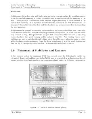
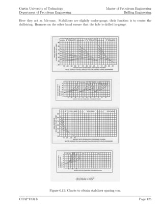

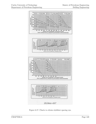
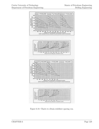
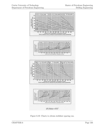
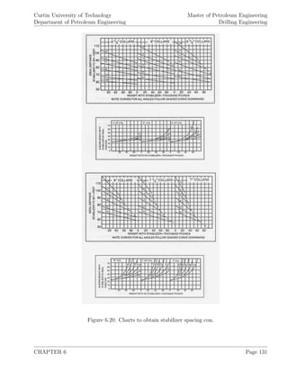
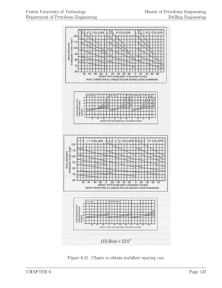
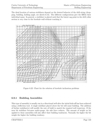
![Curtin University of Technology
Department of Petroleum Engineering
Master of Petroleum Engineering
Drilling Engineering
6.9.2 Holding Assemblies
Once the inclination has been built to the required angle, the tangential section of the well is
drilled using a holding assembly. Holding assemblies do not maintain inclination angle; rather,
they minimize angle build or drop.
Minimal tilt angle at the bit, as well as stiffness of the bottom hole assembly near the bit helps
maintain inclination angle. Change in weight on bit does not affect the directional behavior of this
type of assembly and so optimum weight on bit can be applied to achieve maximum penetration
rates.
6.9.3 Dropping Assemblies
The application of a dropping assembly is that when the inclination has been increased beyond
the intending trajectory and must be reduced to bring the well back on course. Normally these
BHA configurations are more effective in high angled holes. If the hole angle does not decrease,
the weight on bit can be reduced with use of these assemblies, although this will also reduce the
penetration rate.
6.9.4 WOB Increase
Since stabilizers reduce the drillstring tendency to buckle, larger WOBs can be applied. It is
common to express the possible increase in WOB as a percentage of the maximum allowed WOB
without stabilizers. For commonly encountered borehole seizes figure 6.13 can be applied to
derive the proper position of a stabilizer and the resulting bit weight increase when the maximum
allowable WOB without stabilizer is known. This figure is also applied to compare the data to
plan for with practically established data using other combinations of drill collar seize, bit weight,
borehole seize, borehole inclination and formation dip.
In practice, since the ideal position of the stabilizer is based on a particular scenario and the BHAs
are not always changed when the trajectory of the well changes, a compromise when designing the
BHA has to be formed. Therefore the stabilizer is placed between the ideal position, as derived
above and about 10% closer to the bit. When very light weight on bit is run (nonpacked holes),
the stabilizer position should not be closer than 5% to the bit than the ideal position, as it is
calculated above.
6.10 Dogleg Severity Analysis
Dogleg severity is defined as total curvature of the wellbore per 100 [ft] and is expressed with the
unit [◦
/100 ft].
Most of drillpipe failure is caused by fatigue wear, which occurs due to of cycle bending stresses
and axial stresses when the drillpipe under load rotates along a sharp bend (dogleg).
CHAPTER 6 Page 134](https://image.slidesharecdn.com/drillingengineering-160119095813/85/Drilling-engineering-142-320.jpg)
![Curtin University of Technology
Department of Petroleum Engineering
Master of Petroleum Engineering
Drilling Engineering
Since the drilling fatigue is based on the combination of bending and axial stresses as well as
tension in the drillpipe, fatigue danger is highest in the upmost part of the drillstring. Therefore
shallow, sharp bends of the trajectory of deep wells are to be avoided. In these situations rotation
off bottom (no WOB) increases the danger of fatigue wear since the weight of the drill collars
increase the tension load.
To calculate the maximum permissible dogleg severity, equations 6.31 is used:
I =
π
64
. d4
o − d4
i (6.29)
K =
T
E.I
(6.30)
C =
432, 000
π
.
σb
E.D
.
tanh (K.L)
K.L
(6.31)
where:
C [◦
/100 ft] ... maximum permissible dogleg severity
T [lb] ... buoyant weight suspended below the dogleg
(including tool joints)
E [psi] ... Young’s modulus (steel: E = 30.106
[psi])
I [in4
] ... drillpipe moment of inertia
do [in] ... drillpipe outside diameter
di [in] ... drillpipe inside diameter
σb [psi] ... maximum permissible bending stress
D [in] ... drillpipe outer diameter
L [in] ... half the distance between tool joints
(for range 2 drillpipe: 180 [in])
Using the buoyant tensile stress σt [psi], the maximum permissible bending stress σb [psi] can be
found for different grades of drillpipe.
σt =
T
A
(6.32)
Grade E75 drillpipe:
σb = 19, 500 −
10
67
.σt −
0.6
6702
. (σt − 33, 500)2
(6.33)
Grade S135 drillpipe:
CHAPTER 6 Page 135](https://image.slidesharecdn.com/drillingengineering-160119095813/85/Drilling-engineering-143-320.jpg)
![Curtin University of Technology
Department of Petroleum Engineering
Master of Petroleum Engineering
Drilling Engineering
σb = 20, 000 1 −
σt
145, 000
(6.34)
where:
A [in2
] ... cross-sectional area of drillpipe wall
As discussed above, the maximum permissible dogleg severity changes with depth. Therefore a
chart showing maximum permissible dogleg severity on the x-axis and the depth on the y-axis
should be included in the well plan. A sample of such a plot is shown in figure 6.23.
Figure 6.23: Maximum Dogleg Profile
Since lateral loading of tool joints can also create damage to the drillpipe, Lubinski recommended
a maximum lateral load limit of 2,000 [lb] which is expected to not cause damage. Taking lateral
loads F [lbf] into account, the maximum permissible dogleg severity CL [◦
/100 ft] can be calculated
as:
CL =
108, 000.F
π.L.T
(6.35)
CHAPTER 6 Page 136](https://image.slidesharecdn.com/drillingengineering-160119095813/85/Drilling-engineering-144-320.jpg)
![Curtin University of Technology
Department of Petroleum Engineering
Master of Petroleum Engineering
Drilling Engineering
6.11 Examples
1. To drill a well to a depth of 13,500 [ft] using a 5 [in], 19.5 [lb/ft], 4.276 [in] ID grade E and grade
X95 new drillpipe. The total length and weight of the drill collars and heavy-weight drillpipe are
984 [ft] and 157,374 [lb] respectively. The maximum expected mud weight at 12,000 [ft] is 12.5
[ppg]. Calculate the:
(a) Maximum length of each grade of drillpipe that can be used
if a MOP of 50,000 [lb] is to be maintained for the lower grade,
(b) MOP of the heavier grade.
2. A WOB of 50,000 [lb] is to be put on a 12-1
4
[in] bit at a depth of 10,000 [ft]. As assemble, 8
[in] OD, 3 [in] ID, 147 [lb/ft] drill collars are connected to 5 [in], 19.5 [lb/ft] drillpipe. The applied
mud weight is 12.5 [ppg]. What is the required length of drill collars to drill a:
(a) Vertical hole,
(b) Deviated hole with θ = 45◦
3. To run a 4.5 [in] OD liner weighting 50,000 [lb] to 10,000 [ft], a 5 [in] drillpipe, 19.5 [lb/ft],
grade E premium class is used. What is the total stretch of the 8,500 [ft] long drillpipe when the
mud weight is 12.5 [ppg]?
4. Determine the bit weight of the problem data when:
Established data: 7 [in] drill collar OD, 40,000 [lb] WOB, 9 [in] hole seize, 10◦
inclination;
Problem data: 11 [in] drill collar OD, 12 [in] hole seize, 10◦
inclination.
5. What is the ideal stabilizer spacing and percent more bit weight for 8 [in] OD, 3 [in] ID
drill collars when 50,000 [lb] WOB shall be applied on a 12-1
4
bit at a depth of 10,000 [ft]? The
equilibrium angle exists and is kept at 6◦
.
6. A 10,000 [ft] drillstring consists of 9,700 [ft] 5 [in] OD, 4.276 [in] ID, 19.5 [lb/ft], premium
grade E drillpipe and 300 [ft] of 8 [in] OD, 3 [in] ID, 147 [lb/ft] drill collars. The used drilling
mud weight is 12.5 [ppg] and the applied WOB is 45,000 [lb]. What is the maximum permissible
dogleg severity of the drillpipe at 3,000 [ft]?
CHAPTER 6 Page 137](https://image.slidesharecdn.com/drillingengineering-160119095813/85/Drilling-engineering-145-320.jpg)
![Curtin University of Technology
Department of Petroleum Engineering
Master of Petroleum Engineering
Drilling Engineering
7. A drillstring has to be designed using grade E, G and S, premium pipes with OD 5 [in], ID
4.276 [in]. The drill collar used is OD 7 [in], ID 2.5 [in], mud weight applied is 15 [ppg]. When
a minimum of 100,000 [lb] MOP is required, how deep can be drilled? What is the MOP when
drilling at 25,000 [ft]?
CHAPTER 6 Page 138](https://image.slidesharecdn.com/drillingengineering-160119095813/85/Drilling-engineering-146-320.jpg)
![Curtin University of Technology
Department of Petroleum Engineering
Master of Petroleum Engineering
Drilling Engineering
5. Commonly, the mud has to create an overbalanced drilling condition to control the formation
pressure. Mud weight is increased with additives like barite to create a hydrostatic pressure
inside the well which is slightly higher than the formation pressure. Normally, an overbalance
of 100 to 200 [psi] has proven to be adequate to establish safe drilling.
6. Capability to hold drilling cuttings in suspension when circulation is interrupted. Failure of
this capability would allow the cuttings to move down the hole, settle at favorable places
and block the drillstring. This thixotropic capability depends on the individual gel strength
of the drilling mud.
7. To create a buoyance force to partly support the weight of the drillstring and casing string.
The buoyance force is strongly depended on the mud weight used. An increase in mud weight
that increases the buoyance results in smaller surface equipment requirements.
8. Reduce formation damage of various horizons penetrated. The borehole should be drilled
in-gauge (borehole seize = drill bit seize) and either cave-ins (logging and stuck pipe) or wash-
outs (possible cementing problems) avoided. Also the invasion of mud and small cuttings
into the formation or chemical reaction of the mud with the formation have to be avoided
since these would induce a positive skin effect and reduce later production rates.
9. The drilling mud should be neural to the proposed logs run and thus allow to obtain accurate
information about the formations penetrated.
10. The drilling fluid has to transmit the hydraulic horsepower to the bit and allow maximum
penetration rates.
11. The mud system should minimize the torque and drag of the drillstring to decrease wear
and possible failure as well as stuck pipe.
12. For the usage of while drilling tools, the mud should be able to carry the measurement signal
(e.g. as mud pulses).
7.2 Types of Drilling Mud
Out of these different functions, the composition of a particular mud system does depend on
the actual requirements of the individual well or well section. Wells are drilled through different
formations that require different mud properties to achieve optimum penetrations and stable
borehole conditions. Therefore economics, component and additives availability, temperature and
contamination are just a few of the major factors that determine the design of a particular mud
program.
All the possible mixtures that form drilling mud can be generally characterised by the following
system. Further sub-classifications do exist.
CHAPTER 7 Page 140](https://image.slidesharecdn.com/drillingengineering-160119095813/85/Drilling-engineering-148-320.jpg)

![Curtin University of Technology
Department of Petroleum Engineering
Master of Petroleum Engineering
Drilling Engineering
To control corrosion, hydrogen embrittlement and the solubility of Ca2+
and Mg2+
, a high pH
value is required and can be controlled with caustic (NaOH).
Clear Water and Native Muds
To drill compact formations which are normally pressured (formation pressure equals hydrostatic
pressure caused by formation fluids), fresh water and salt-saturated water can be used as drilling
mud. As the name indicates, native muds are a mixture of water and clays or shales from the
cuttings drilled. Here the clays or shales are dissolved by the water and returned to the surface.
Clear water and native muds are the cheapest mud systems since no additional material to form
the mud is needed. They are also environmentally best accepted.
Inhibitive water-base Mud – Calcium Muds
When swelling and hydration of clays and shales are expected, inhibitive water-base muds can be
applied. Calcium muds are best suited to penetrate horizons that contain gypsum and hydrite. A
subclassification of inhibitive water-base muds distinguishes seawater muds, saturated saltwater
muds, lime muds and gypsum muds.
Dispersed Muds – Lignosulphonate Muds
Dispersed muds are used when the mud has to have following characteristics: relative high mud
weight (larger than 14 [ppg]), used at moderately high formation temperatures, low filtration loss
required and high tolerance for contamination by drilling solids.
Some of the disadvantages when using dispersed muds are: heaving of shales and causing formation
damage due to dispersant of formation clays in the presence of lignosulphonate.
Dispersed mud systems consist of: fresh or salty water, bentonite, lignosulphonate, caustic soda
and colloidal polymers (carboxy methyl cellulose or stabilized starch). In general, these mud
systems exhibit better control of viscosity, a higher solids tolerance and a better control of filtration
than nondispersed muds.
Nondispersed Muds – KCL/Polymer Muds
To drill water sensitive and sloughing shales such as productive sands which are prone to formation
damage, fresh water nondispersed muds are applied. Commonly, nondispersed muds are associated
with low mud weights and low solid concentrations.
Nondispersed mud systems consist of: fresh water or brine, potassium chloride (KCl), inhibiting
polymer, viscosifier, stabilized starch or carboxy methyl cellulose, caustic soda and lubricants.
CHAPTER 7 Page 142](https://image.slidesharecdn.com/drillingengineering-160119095813/85/Drilling-engineering-150-320.jpg)
![Curtin University of Technology
Department of Petroleum Engineering
Master of Petroleum Engineering
Drilling Engineering
Low-solids polymer mud systems are widespread in the industry since they offer advantages like
increased penetration rate, hole stability, shear thinning ability, hole cleaning with maximum
hydraulics and lower equivalent circulation density over conventional deflocculated muds. With
all these advantages, they also have disadvantages like instability at temperatures above 250 [F],
irreversible absorption of the polymer on clay, a higher dilution and an adequate solids removal
equipment is required as well as they are more corrosive.
Flocculated Muds
Flocculated muds posses generally a dynamic increase in filtration, viscosity and gel strength.
Flocculation refers to a thickening of the mud due to edge-to-edge and edge-to-face association
of clay particles. The flocculation is commonly caused by high active solids concentration, high
electrolyte concentration and high temperature. To reduce the flocculating tendency of the mud,
chemical additives, also called deflocculants or thinners are used. Thinners like phosphates, tan-
nins, lignins and lignosulphonate are applied to lower the yield point and gel strength. When
deflocculants are added, the pH-value is controlled by NaOH.
Salt-saturated Muds
Salt-saturated muds are used to drill through salt domes and salt sections. These mud systems are
saturated with sodium chloride (NaCL) that prevents severe hole enlargements due to washouts
of the salt formations. Swelling of bentonitic shales is controlled by adding of polymer.
7.2.2 Oil-base Muds
Opposite to water-base muds where water is the continuous phase, at oil-base mud systems crude
or diesel oil forms the continuous phase in the water-in-oil emulsion. In this way oil-base mud can
have as little as 3% to 5% or as much as 20% to 40% (invert emulsions) water content. Oil-base
mud systems are applied when:
1. Drilling sensitive production zones or problem shales,
2. Drilling salt sections and formations that contain hydrogen sulfide,
3. Danger of stuck pipe problems,
4. Drilling at bottom hole temperatures that are permissable by water-base muds.
Low-gravity solids content has to be monitored closely when drilling with oil-base muds since
at this environment solids do not hydrate which causes low-gravity solids contents to exceed
acceptable levels often. This results in reduction of penetration rate, formation damage and
increase in risk of differential sticking.
CHAPTER 7 Page 143](https://image.slidesharecdn.com/drillingengineering-160119095813/85/Drilling-engineering-151-320.jpg)
![Curtin University of Technology
Department of Petroleum Engineering
Master of Petroleum Engineering
Drilling Engineering
Since oil-base muds contain substantially less colloidal particles, they exhibit a spurt fluid loss.
Due to the higher filtration rates, the monitoring of high-pressure high-temperature filtration as
well as the drilling conditions are important to ensure that excessive filtration or filter cake buildup
does not lead to problems.
7.3 Mud Calculations
The fundamental properties to describe a drilling mud are:
1. Mud weight,
2. Plastic viscosity,
3. Yield point,
4. Gel strength,
5. Filtrate and filter cake,
6. pH-value.
The procedures and equations to calculate the rheological properties like the plastic viscosity, the
yield point and the gel strength were discussed at drilling hydraulics. In the following, the reaming
mud characteristics and their measurement in the field are elaborated.
pH Determination
The pH-vale is defined as negative logarithm of the hydrogen ion content of a solution (pH =
− log[H+
]). In this way, an increase of the concentration of H+
ions decreases the pH-value and a
decrease of H+
ions increases the pH-value. When the pH-value is known, it is determined whether
the mud is acidic (OH−
< H+
thus pH-value < 7) or alkaline (OH−
> H+
, thus pH-value > 7). A
pH-value of 7 indicates a neutral mud.
Measuring the pH-value of a fluid is either performed with the help of a pH-meter or a special
pH-paper which changes color according to the pH-value determined.
The OH−
concentration within a solution, at a given pH-value, is defined by:
H+
OH−
= 1.0.10−4
(7.1)
or:
OH−
= 10(pH−14)
(7.2)
CHAPTER 7 Page 144](https://image.slidesharecdn.com/drillingengineering-160119095813/85/Drilling-engineering-152-320.jpg)
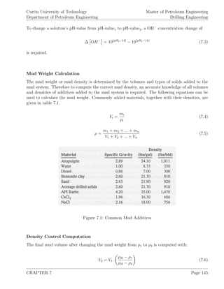
![Curtin University of Technology
Department of Petroleum Engineering
Master of Petroleum Engineering
Drilling Engineering
In practice, since excess storage capacity is not available and to limit the amount of added, costly
weighting material, before the density is increase (e.g. by adding barite), some mud volume is
discarded from the circulation system. In this situation, equation 7.7 calculates the volume the
existing mud has to be reduced to before weighting material is added:
V1 = V2.
ρB − ρ2
ρB − ρ1
(7.7)
With the knowledge of the volumes, the densities of the original mud and the weighting material,
the weight of barite required is given by:
mB = 42. (V2 − V1) .ρB (7.8)
where:
mB [lbm] ... weight of API barite
ρB [ppg] ... density of API barite
ρ1 [ppg] ... density of original mud before weighting
ρ2 [ppg] ... density of final mud after weighting
V1 [bbl] ... volume of original mud before weighting
V2 [bbl] ... volume of final mud after weighting
Due to the barite’s extremely large surface area, barite has the tendency to adsorb a large amount
of water from the mud system and thus increases the viscosity of the drilling mud.
This thickening is avoided when not only barite but also a minimum amount of water, to wet the
barite, is added simultaneously. A common practice is to add 1 [gal] of water for each added 100
[lbm] of barite. To take this extra water into account and when assuming that original mud is
discarded before weighting, following equations give the volume of original mud and the amount
of barite required:
V1 =
ρB
1+ρw.VwB
1+ρB.VwB
− ρ2
ρB
1+ρw.VwB
1+ρB.VwB
− ρ1
(7.9)
mB =
42.ρB
1 + ρB.VwB
. (V2 − V1) (7.10)
where:
VwB [gal/lb] ... volume of water added with barite
ρw [ppg] ... density of water added with barite
CHAPTER 7 Page 146](https://image.slidesharecdn.com/drillingengineering-160119095813/85/Drilling-engineering-154-320.jpg)
![Curtin University of Technology
Department of Petroleum Engineering
Master of Petroleum Engineering
Drilling Engineering
When the concentration of low-gravity solids should be kept to a minimum value (see comments
before), it is cheaper to reduce them by dilution before weighting the original mud with barite.
The following equations are applied to calculate the corrected volume of the original mud V1, the
volume of the dilution water Vw, the mass of the weighting material m2 and the obtained final
mud volume V2 after weighting:
V1 = V2.
fc2
fc1
(7.11)
Vw =
(ρB − ρ2) .V2 − (ρB − ρ1) .V1
(ρB − ρw)
(7.12)
mB = 42. (V2 − V1 − Vw) .ρB (7.13)
Solids Control for Weighted Muds
Solids control in general is the separation of drilling fluid, heavy solids and lighter components. To
perform this separation, centrifuges are used along with other surface equipment, see description
of the circulation system. In the following, the function of the centrifuge shall be evaluated to
some extend.
After degasification and run over various screens as well as a separation tank to discard formation
gas and cuttings from the mud, the mud is fed into a centrifuge. The centrifuge discharges at an
“underflow” a high-density slurry (ρu) containing API barite, and at an “overflow” a low-density
slurry (ρo) containing low-gravity solids, water and some chemicals. The overflow with its low-
density slurry is discarded from the circulation system, the underflow with the high-density slurry
is returned to the active mud system.
With equation 7.14 the flow rate of the underflow is computed as:
qu =
qm. (ρm − ρo) − qw1. (ρo − ρw)
(ρu − ρo)
(7.14)
where:
ρu [ppg] ... density of the underflow slurry
ρo [ppg] ... density of the overflow slurry
qu [gpm] ... underflow flow rate
qw1 [gpm] ... flow rate of dilution water entering the centrifuge
qm [gpm] ... flow rate of drilling fluid entering the centrifuge
ρm [ppg] ... density of drilling fluid entering the centrifuge
ρw [ppg] ... density of dilution water entering the centrifuge
CHAPTER 7 Page 147](https://image.slidesharecdn.com/drillingengineering-160119095813/85/Drilling-engineering-155-320.jpg)
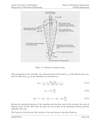
![Curtin University of Technology
Department of Petroleum Engineering
Master of Petroleum Engineering
Drilling Engineering
fm =
qu.fum
qm
(7.18)
To maintain the desired mud concentration [lb/bbl] at the mixing pit, the individual mass rates
of the mud additives are calculated as:
wi = ci.qm.
(1 − fm)
42
= ci
(qm − qu.fum)
42
(7.19)
where:
qm [gal/min] ... flow rate of the mud
qu [gal/min] ... flow rate of the underflow
ci [lb/bbl] ... desired concentration of the ith additive
of the mud stream
42 [gal/bbl] ... conversion [gal] -> [bbl]
Figure 7.3: Sketch of a mud-cleaner
To keep the density of the mud leaving the mixing pit equal to the density of the mud feeded to
the centrifuge, the required water flow rate and the mass rate of API barite are computed with:
CHAPTER 7 Page 149](https://image.slidesharecdn.com/drillingengineering-160119095813/85/Drilling-engineering-157-320.jpg)
![Curtin University of Technology
Department of Petroleum Engineering
Master of Petroleum Engineering
Drilling Engineering
qw2 =
qm. (ρB − ρm) − qu. (ρB − ρu) − wc
ρB
ρc
− 1 − n
i=1 wi. ρB
ρi
− 1
(ρB − ρw)
(7.20)
wB = qm − qu − qw2 −
wc
ρc
−
n
i=1
wi
ρi
.ρB (7.21)
where:
wc [lbm/min] ... mass flow rate of clay and deflocculant
ρc [ppg] ... density of clay and deflocculant
7.4 Recommended Mud Flow Properties
In the following, empirical correlations to compute the recommended upper and lower limits of the
plastic viscosity and the yield point are given in table 7.4. It should be noted that all correlations
below are based on mud densities only.
Figure 7.4: Limits of plastic viscosity and yield point
The recommended maximum total solids percentage fST and the percentage of low-gravity solids
flg are computed with:
CHAPTER 7 Page 150](https://image.slidesharecdn.com/drillingengineering-160119095813/85/Drilling-engineering-158-320.jpg)
![Curtin University of Technology
Department of Petroleum Engineering
Master of Petroleum Engineering
Drilling Engineering
fST = 2.917.ρm − 14.17 (7.22)
flg =
100. (8.33 − ρm + 26.67.fST )
13.3
(7.23)
where:
ρm [ppg] ... mud density
CHAPTER 7 Page 151](https://image.slidesharecdn.com/drillingengineering-160119095813/85/Drilling-engineering-159-320.jpg)
![Curtin University of Technology
Department of Petroleum Engineering
Master of Petroleum Engineering
Drilling Engineering
7.5 Examples
1. The pH-value of a drilling fluid is to be raised from 8 to 11.5. What is the amount of caustic,
having a molecular weight of 40 required?
2. When 150 [lbm] of API barite, 40 [lbm] of bentonite and 1 [bbl] of water are mixed, what is
the resulting density?
3. When 70 [lbm] of calcium chloride is mixed with 1 [bbl] of water, what is the resulting density?
4. 700 [bbl] of mud have to be increased in density from 13 [ppg] to 15 [ppg] by adding of API
barite. Since the mud thickness has to be maintained, 1 [gal] of water is added with every 100 [lb]
of barite. Calculate the total amount of water and barite required when there is no limitation in
the final volume.
5. When 1,000 [bbl] of mud have to be increased from 10 [ppg] to 13 [ppg] mud weight by adding
API barite, the total volume is limited to 1,000 [bbl]. How much old mud has to be discarded and
what is the weight of the added API barite?
6. Using the data from example 5., the volume fraction of low-gravity solids must be reduced
from 0.06 to 0.035 by adding water. Compute the API barite and water to be added as well as
the amount of old mud to be discarded.
7. A centrifuge is fed by a 15 [ppg] mud and 8.33 [ppg] dilution water at rates of 30 [gpm] and 15
[gpm] respectively. The overflow has a density of 11 [ppg], the underflow 25 [ppg]. Assuming that
the mud contains 30 [lb/bbl] bentonite and 15 [lb/bbl] deflocculant, determine the rates to add
bentonite, deflocculant, water and API barite to maintain the mud properties at the mixing pit.
CHAPTER 7 Page 152](https://image.slidesharecdn.com/drillingengineering-160119095813/85/Drilling-engineering-160-320.jpg)
![Curtin University of Technology
Department of Petroleum Engineering
Master of Petroleum Engineering
Drilling Engineering
Chapter 8
Casing Design
Casing costs compromise one of the largest cost items of the drilling project. Therefore propper
planning of casing setting depths and casing selection is vital to realise a cost effective and safe
well. The casings themselves fulfill multiple functions that can be summarized as:
1. Isolate porous formations with different fluid-pressure regimes from contaminating the pay
zone,
2. Prevent near surface fresh water zones from contamination with drilling mud,
3. Protect the hole from caving in,
4. Provide a connection and support of the wellhead equipment,
5. Provide exact dimensions for running testing, completion and production subsurface equip-
ment.
8.1 Casing Types
According to the different functions, the total casing program consists of different casings strings.
8.1.1 Conductor Casing
The function of the conductor is to enable circulation of the drilling fluid to the shale shakers
without eroding the surface sediments directly below the rig foundation. The conductor prevents
the subsequent casings from corrosion and may partly support the wellhead weight.
Commonly a diverter is installed on top of the conductor casing to divert an unexpected inflow of
formation fluids into the wellbore away from the rig-site and the personal.
Conductor setting depths are in the range of 150 to 600 [ft], their seizes range from 36 to 20 [in].
CHAPTER 8 Page 153](https://image.slidesharecdn.com/drillingengineering-160119095813/85/Drilling-engineering-161-320.jpg)
![Curtin University of Technology
Department of Petroleum Engineering
Master of Petroleum Engineering
Drilling Engineering
8.1.2 Surface Casing
Figure 8.1: Casing program
The function of the surface casing is to prevent cave
in of unconsolidated, weak near-surface formations as
well as protect the shallow, freshwater sands from con-
tamination with drilling mud. As the conductors, sur-
face casing protects the subsequent casings from cor-
rosion.
Before the surface casing is set, no blow out preventers
(BOP) are installed. After setting the surface casing
and installing the wellhead, a BOP is available to han-
dle kicks when drilling the intermediate hole section.
Surface casing setting depths are in the range from
300 to 5,000 [ft], their diameters range from 24 to 17-
1
2
[in]. Note that the surface casing setting depth is
often determined by government or company policy
and not selected due to technical reasoning.
8.1.3 Intermediate Casing
The intermediate casing string is a purely technical
casing. One or more may be necessary to handle
abnormal formation pressures, unstable shale forma-
tions, lost circulation or cave-in zones. An intermedi-
ate casing may also be necessary to realize the planned
mud weight profile. When for example an abnormally
pressured formation is encountered, it may have to
be protected by an intermediate casing so when for-
mation pressure of the formations below is normal, a
lower mud weight can be applied. Intermediate casing
diameters range from 17-1
2
to 9-5
8
[in].
8.1.4 Production Casing
The production casing is set through the prospective
production zone(s). This casing string protects the
environment in case of production tubing failure and
permits the tubing string to be maintained or replaced
during the production life. Commonly production cas-
ing and production liners have gas-tight connections,
their diameters range from 9-5
8
to 5 [in]. A production
casing diameter of 7 [in] is encountered often.
CHAPTER 8 Page 154](https://image.slidesharecdn.com/drillingengineering-160119095813/85/Drilling-engineering-162-320.jpg)
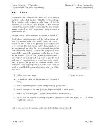
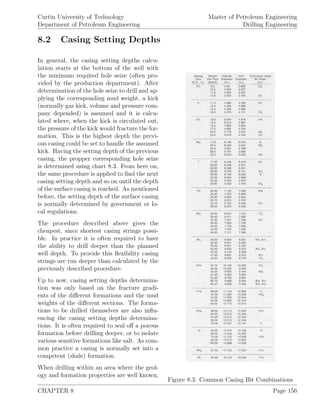
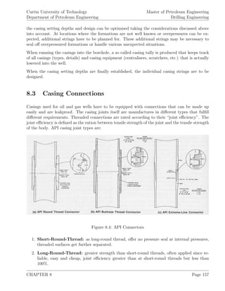
![Curtin University of Technology
Department of Petroleum Engineering
Master of Petroleum Engineering
Drilling Engineering
3. Buttress-Thread: offers a nearly 100% joint efficiency, is not 100% leakproof.
4. Extreme-Line: design is an integral joint (box is matched on the pipe wall), pipe wall
must be thicker near the ends of the casing to provide the necessary strength, OD of this
connection is significantly lower than of others and half as many threaded, connections exist,
metal-to-metal seal, much more expensive.
Since round-threads have eight threads per [in], they are sometimes called API 8-Round threads
as well.
Figure 8.5: Typical Casing Programs
Along with these API connection types, other ones offering premium features are applied in the
industry. Some of these special features are:
1. Flush joints for maximum clearance.
2. Smooth bores through connectors for reduced turbulence.
3. Threads designed for fast make-up with low tendency to cross-thread.
4. Multiple metal-to-metal seals for enhanced pressure integrity.
5. Multiple shoulders for enhanced torque strength.
6. High compressive strengths for special loading situations.
7. Resilient rings for secondary pressure seals and connector corrosion protection.
CHAPTER 8 Page 158](https://image.slidesharecdn.com/drillingengineering-160119095813/85/Drilling-engineering-166-320.jpg)
![Curtin University of Technology
Department of Petroleum Engineering
Master of Petroleum Engineering
Drilling Engineering
As drillpipes, casings are manufactured in different length ranges:
Range 1 16 to 25 [ft],
Range 2 25 to 34 [ft],
Range 3 34 to 48 [ft],
8.4 API Casing Performance Properties
The American Petroleum Institute (API) has developed internationally accepted standards for
oilfield tubulars and summarised them in bulletins that contain the minimum performance prop-
erties and equations to compute these properties. It should be understood that these properties
are guidelines (minimum requirements), for casing design calculations, the exact strength values
provided by the individual manufacture shall be applied.
A casing is defined by:
1. Casing outside diameter (OD),
2. Weight per unit length (this determines the wall thickness),
3. Grade of steel,
4. Type of coupling,
5. Length of joint.
To determine the strength of various casing materials, API has designated defined grades. The
grading code consists of a letter followed by a number where the number gives the minimum yield
strength of the material in thousands of [psi], the number is an arbitrary one (e.g. N-80). For wells
that require very high tensile strength, collapse resistance or better corrosion resistance, non-API
casings are used by the industry as well.
Tables 8.6 through 8.21 list API and some non-API ones as well as gives the minimum performance
properties of them. To calculate the individual properties following equations can be applied:
Yield strength collapse pressure:
py = 2.σy
do
t
− 1
(do
t
)2
(8.1)
Above equation is valid up to where do
t
intersects (do
t
)yp and thus the plastic deformation starts.
(do
t
)yp is calculated as:
CHAPTER 8 Page 159](https://image.slidesharecdn.com/drillingengineering-160119095813/85/Drilling-engineering-167-320.jpg)
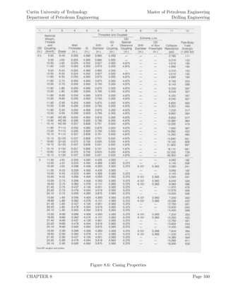
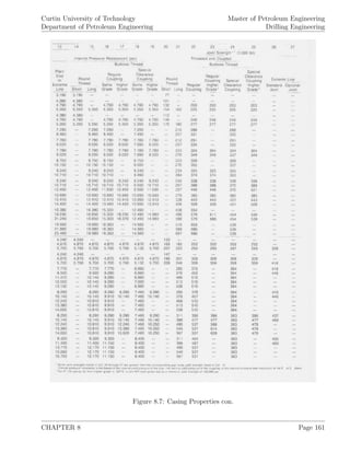
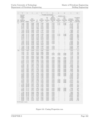
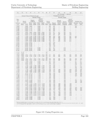
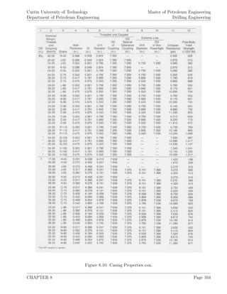
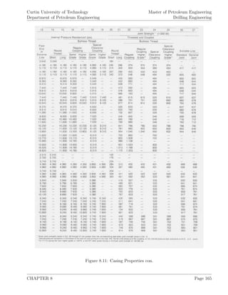
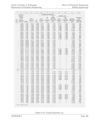
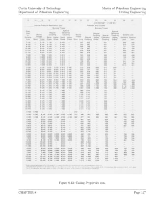
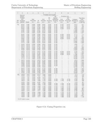
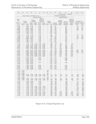
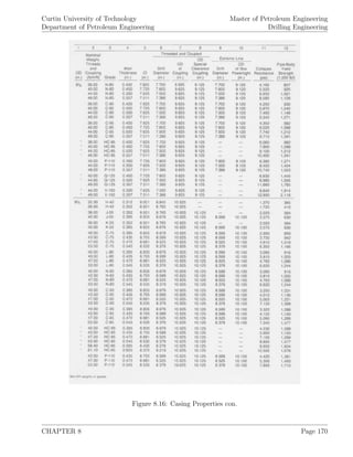
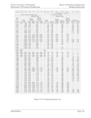
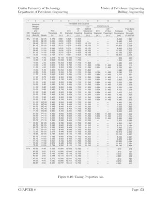
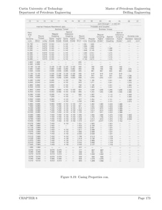
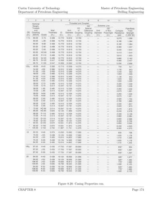
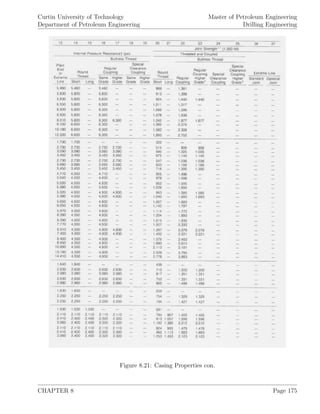
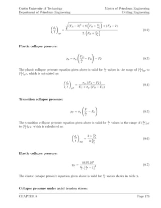
![Curtin University of Technology
Department of Petroleum Engineering
Master of Petroleum Engineering
Drilling Engineering
σya = 1 − 0.75 (σa − σy)2
− 0.50.
σa
σy
.σy (8.8)
Pipe body yield strength
Wp = 0.7854. d2
o − d2
i σy (8.9)
Round thread casing joint strength - short & long threads & couplings:
Lesser of
Wj = 0.95.Aip.σup (8.10)
and
Wj = 0.95.Aip.Le
0.74.d−0.59
o .σup
0.5.Le + 0.141.do
+
σy
Le + 0.141.do
(8.11)
Buttress thread casing joint strength:
Lesser of
Wj = 0.95.Ap.σup. 1.008 − 0.0396. 1.083 −
σy
σup
(8.12)
and
Wj = 0.95.Ac.σuc (8.13)
Casing types can be normally identified by their nominal weight, which are based on 20 [ft] length
of threaded and coupled casing joint. They can are calculated as:
Nominal casing weight:
Wn = 10.68. (do − t) .t + 0.0722.d2
o (8.14)
The plain end casing weight is defined as the weight of the casing joint without inclusion of threads
and couplings.
CHAPTER 8 Page 177](https://image.slidesharecdn.com/drillingengineering-160119095813/85/Drilling-engineering-185-320.jpg)
![Curtin University of Technology
Department of Petroleum Engineering
Master of Petroleum Engineering
Drilling Engineering
Plain end casing weight:
Wpe = 10.68. (do − t) .t (8.15)
where for all equations above,
do [in] ... tubular outside diameter
t [in] ... tubular wall thickness
σy [psi] ... minimum yield pressure of tubular
σya [psi] ... yield strength of axial stress equivalent grade
σa [psi] ... axial stress-tension (positive)
FA ... correlation factor, given in table 8.22
or:
FA = 2.8762 + 0.10679.10−5
.σy + 0.21301.10−10
.σ2
y − 0.53132.10−16
.σ3
y (8.16)
FB ... correlation factor, given in table 8.22
or:
FB = 0.026233 + 0.50609.10−6
.σy (8.17)
FC ... correlation factor, given in table 8.22
or:
FC = −465.93 + 0.030867.σy − 0.140483.10−7
.σ2
y + 0.36989.10−13
.σ3
y (8.18)
FF ... correlation factor, given in table 8.22
or:
FF =
46.95.106
. (3FB/FA/2 + FB/FA)3
σy. (3FB/FA/2 + FB/FA − FB/FA) . (1 − 3FB/FA/2 + FB/FA)2 (8.19)
FG ... correlation factor, given in table 8.22
CHAPTER 8 Page 178](https://image.slidesharecdn.com/drillingengineering-160119095813/85/Drilling-engineering-186-320.jpg)
![Curtin University of Technology
Department of Petroleum Engineering
Master of Petroleum Engineering
Drilling Engineering
or:
FG =
FF .FG
FA
(8.20)
Figure 8.22: Empirical coefficients for collapse pressure calculations
Aip [in2
] ... cross-sectional area of the tubular wall under
the last perfect thread
Ap [in2
] ... cross-sectional area of plain end tubular
Ac [in2
] ... cross-sectional area of coupling
Le [in] ... engaged thread length
σup [psi] ... minimum ultimate strength of tubular
σuc [psi] ... minimum ultimate strength of coupling
8.5 General Casing Design Criteria
Casing design itself is an optimization process to find the cheapest casing string that is strong
enough to withstand the occurring loads over time. The design itself is therefore depended on:
CHAPTER 8 Page 179](https://image.slidesharecdn.com/drillingengineering-160119095813/85/Drilling-engineering-187-320.jpg)
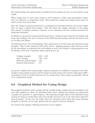
![Curtin University of Technology
Department of Petroleum Engineering
Master of Petroleum Engineering
Drilling Engineering
Burst line:
1. Calculate the external pressure due to an assumed fluid column of 0.465 [psi/ft] (salt-
saturated completion fluid),
2. Calculate the internal pressure due to the maximum anticipated pressures when drilling the
next section,
3. Calculate the burst pressure pb as the difference between the external and the internal
pressures,
pb = pf − (TD − CSD) .Gf − 0.053.ρm.CSD (8.24)
where:
pf [ft] ... maximum anticipated formation pressure to drill next section
TD [ft] ... total depth (TVD)
CSD [ft] ... casing setting depth (TVD)
Gf [psi/ft] ... formation fluid gradient
ρm [ppg ... mud density
In this way the burst pressure at the surface is calculated as:
pb = pf − TD.Gf (8.25)
4. On the pressure vs. depth graph draw a stright line between the maximum Burst pressure
at the casing top and the minimum burst pressure at the casing shoe,
5. Select from tables 8.6 through 8.21 casings with burst resistance above the burst loading
line,
6. Draw the vertical lines of the casings with the individual grades,
7. The individual intersections of the burst loading line and the casing burst resistances deter-
mine the depths from which upwards the casing grades can be used.
Collapse line:
1. Calculate the external and internal pressure due to the mud columns outside and inside the
casing,
2. Calculate the collapse pressure pc as the difference between the external and the internal
pressures,
CHAPTER 8 Page 182](https://image.slidesharecdn.com/drillingengineering-160119095813/85/Drilling-engineering-190-320.jpg)
![Curtin University of Technology
Department of Petroleum Engineering
Master of Petroleum Engineering
Drilling Engineering
3. On the pressure vs. depth graph draw a stright line between the maximum collapse pressure
at the casing shoe and the zero at the casing top,
4. Select from tables 8.6 through 8.21 casings with collapse resistance above the collapse loading
line,
5. Draw the vertical lines of the casings with the individual grades,
6. The individual intersections of the collapse loading line and the casing collapse resistances
determine the depths up to the casing grades can be used.
Tensile line:
1. Calculate the weight of the casing string in air,
2. Calculate the buoyancy force,
3. Calculate the bending force with equation 8.26 when designing the casing for a deviated
hole,
BF = 63.doWcs.θ (8.26)
where:
BF [lbf] ... bending force
θ [◦
] ... change of angle in deviation
Wcs [lb/ft] ... nominal weight of casing Wcs = 3.46.Acs
4. Calculate shock loads due to setting of the casing using equation 6.18 by replacing Wdp with
Wcs,
5. Draw tensile loading on the pressure vs. depth graph,
6. Select casings from table x that have higher body yield strength than the tensile loading,
Having drawn all three major design criteria within one plot, a combined casing sting that is
strong enough at all depth can be selected. Finally check that the joint strengths are larger the
the calculated tensile loading.
Note that this procedure for casing design considers strength criteria only and is not optimized
for real casing costs. Thus a stronger casing might be preferred since it is cheaper (availability,
etc.) than a weaker one.
CHAPTER 8 Page 183](https://image.slidesharecdn.com/drillingengineering-160119095813/85/Drilling-engineering-191-320.jpg)
![Curtin University of Technology
Department of Petroleum Engineering
Master of Petroleum Engineering
Drilling Engineering
Figure 8.23: Sketch of graphical design of a casing string
8.7 Maximum Load Casing Design for Intermediate Cas-
ing
The load criteria assumed above are based on a 100 % empty casing (collapse) and a 100 % gas-kick
filled (burst) one respectively. These are very conservative assumptions that lead to over-design
causing unnecessary high cost of the casing string. If standard drilling procedures and precautions
are followed, these assumptions are not to be expected. When drilling into a weak or fractured
formation that causes lost circulation, the remaining fluid hight can be estimated with:
L =
0.465.CSD
ρm.19.25
(8.27)
where:
ρm [ppg] ... weight of mud used to drill next section.
For this reason the casing is supported in the inside by the hydrostatic pressure of the remaining
mud column of length L.
CHAPTER 8 Page 184](https://image.slidesharecdn.com/drillingengineering-160119095813/85/Drilling-engineering-192-320.jpg)
![Curtin University of Technology
Department of Petroleum Engineering
Master of Petroleum Engineering
Drilling Engineering
In case of burst, the conservative assumption can be relaxed with the assumption that the gas-kick
will fill between 40% to 60% of the hole before the well is shut in and steps to circulate the kick
out are taken. Modern kick detection systems detect kicks of 20 [bbl] and below (depending on
the hole seize) and thus the assumption above could be even more relaxed.
8.8 Casing Centralizer Spacings
To have a centered casing string which is essential for proper cementing and to lower dragging
forces when running the casing, so called centralizers are placed along the casing string. The
clearance (distance between casing OD and wall) is called “standoff”. The centralizer spacing
should be sufficient enough to provide a minimum standoff but excessive use of them do induce
additional drag, can disturb the cement flow and, last but not least, add to the well costs.
Figure 8.24: Casing centralizers
In normal oilfield services, following equations are used:
(WF)b = Wcs + 0.0408. ρmi.d2
i − ρmo.d2
o (8.28)
T = 0.0408.TV D. ρmi.d2
i − ρmo.d2
o . cos θ.Wcs.S (8.29)
CHAPTER 8 Page 185](https://image.slidesharecdn.com/drillingengineering-160119095813/85/Drilling-engineering-193-320.jpg)
![Curtin University of Technology
Department of Petroleum Engineering
Master of Petroleum Engineering
Drilling Engineering
CS =
F
0.0175.T.DLS + (WF)b . sin θ
(8.30)
F = 2.T. sin DLS.
CS
2
+ (WF)b .CS. sin θ (8.31)
where:
F [lbf] ... force on each centralizer
CS [ft] ... spacing of centralizer
Wcs [lb/ft] ... nominal weight of casing
θ [◦
] ... average inclination angle near the centralizer
T [lbf] ... tension in the casing at centralizer
TV D [ft] ... true vertical depth to the casing shoe
ρmi [ppg] ... mud weight inside the casing
ρmo [ppg] ... mud weight outside the casing
S [ft] ... distance of the centralizer from the casing shoe.
DLS [◦
/100 ft] ... dogleg severity
di [in] ... inside diameter of the casing
do [in] ... outside diameter of the casing
S [ft] ... distance of casing shoe to particular centralizer
To control vertical travel of the centralizers, casing couplings or various types of attached stops
are applied.
8.9 Stretch in Casing
The elongation or stretch of tubular material resulting from pulling forces and its own weight is
part of the design calculation. As it can easily be understood, the amount of stretch depends on
the amount of pull, the length of the tubular, the elasticity of the material and its cross-sectional
area. Following equations can be applied to calculate the tubular elongation:
Tubular freely suspended in fluid:
∆Lt = ∆L1 + ∆L2 + ∆L3 + F1.
W2 + W3
W1
+ F2.
W3
W2
+
C1. [Ls1.Ls2 + (Ls1 + Ls2) .Ls3] − C2 L2
s2.
W1
W2
+ L2
s3.
W1 + W2
W3
(8.32)
The tension stresses along the casing string after setting and cementing are given by:
CHAPTER 8 Page 186](https://image.slidesharecdn.com/drillingengineering-160119095813/85/Drilling-engineering-194-320.jpg)
![Curtin University of Technology
Department of Petroleum Engineering
Master of Petroleum Engineering
Drilling Engineering
Wt = 1 −
ρm
ρs
. (w1.L1 + w2.L2 + ... + wn.Ln) (8.33)
Lo = 1.36.10−6
.Wt
L1
w1
+
L2
w2
+ ... +
Ln
wn
(8.34)
Ls = 4.0.10−7
.σt.L (8.35)
where:
∆Lt [in] ... total axial stretch or contraction
∆L1 [in] ... stretch corresponding to length Ls1
F1 [in] ... free stretch factor corresponding to length Ls1
Wn [lbs] ... weight of the nth string
wn [lb/ft] ... weight of nth section above top of cement
Ln [ft] ... length of nth section above top of cement
Wt [lbs] ... total load below top of cement
Ls [in] ... stretch corresponding to tension σt
σt [psi] ... tension stress desired to be left at top of cement
Lo [in] ... distance required to lower top of casing for
zero stress at top of cement
Ld [in] ... distance to lower top of casing for a desired stress
at the top of cement
The factors ∆Ln and Fn are obtained from figure x where:
C1 = 1.20177.10−7
for salt water
C1 = 1.50869.10−7
for common mud
C1 = 0 for air.
C2 = 2.00294.10−7
for salt water
C2 = 2.51448.10−7
for common mud
C2 = 0 for air.
L = L1 + L2 + ... + Ln (8.36)
Ld = Lo − Ls (8.37)
Single-weight string suspended in mud:
CHAPTER 8 Page 187](https://image.slidesharecdn.com/drillingengineering-160119095813/85/Drilling-engineering-195-320.jpg)
![Curtin University of Technology
Department of Petroleum Engineering
Master of Petroleum Engineering
Drilling Engineering
Lo = 1.1085.10−5
. (D − L ) (8.38)
where:
D [ft] ... total depth of the well or length of the string
L [ft] ... length of casing below top of cement.
CHAPTER 8 Page 188](https://image.slidesharecdn.com/drillingengineering-160119095813/85/Drilling-engineering-196-320.jpg)
![Curtin University of Technology
Department of Petroleum Engineering
Master of Petroleum Engineering
Drilling Engineering
8.10 Examples
1. A 20 [in] conductor pipe is set in a 26 [in] hole at 400 [ft]. The mud weights for this well are
8.69 [ppg] to drill the conductor and 8.96 [ppg] for the next section, a 17-1
2
[in] hole reaching 6,250
[ft]. Design the conductor using 0.85 for collapse safety factor, 1.1 for burst safety factor and 1.8
for the tension safety factor.
2. Continuing from example 1, design the 13-3
8
[in] intermediate casing which is run until 6,250
[ft]. The next hole section is drilled with a 9.8 [ppg] mud to a depth of 10,000 [ft].
3. Continue from example 1 and 2, the 9-5
8
[in] casing, set at 10,000 [ft] is to be designed. Thereto
a kick at 13,000 [ft] causes from a formation pressure of 0.57 [psi/ft] is assumed. The mud weight
used to drill until 13,000 [ft] is 11.5 [ppg], the maximum dogleg severity at the hole is 3 [◦
/ 100
ft]. Following casings shall be assumed to be available for this well:
Grade: Weight [lb/ft] Collapse [psi] Burst [psi]
C-75 43.5 3,750 5,930
L-80 47.0 4,750 6,870
C-95 53.5 7,330 9,410
4. Re-design the 9-5
8
[in] casing applying the released assumptions that a remaining mud is left
inside the hole and the kick fills the well bore to 50 % before shut in.
5. A well is to be drilled to 10,000 [ft] MD (4,200 [ft] TVD). At the gradual dogleg of the section
6,020 [ft] with an inclination of 38◦
and a direction of N3◦
and 6,220 [ft], showing an inclination
of 46◦
and a direction of N7E◦
, a centralizer is to be placed. To maintain a standoff of 1 [in]
while bearing a wall force of 1,100 [lbf], the centralizer spacing is to be designed. ρmo = 12 [ppg],
ρmi = 15 [ppg], Wcs = 53 [lb/ft], do = 9.625 [in], di = 8.535 [in]
CHAPTER 8 Page 189](https://image.slidesharecdn.com/drillingengineering-160119095813/85/Drilling-engineering-197-320.jpg)

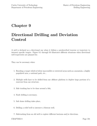
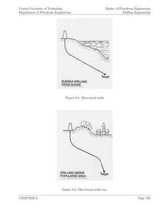
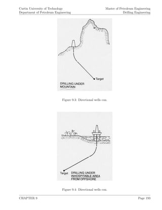
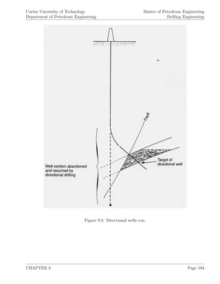
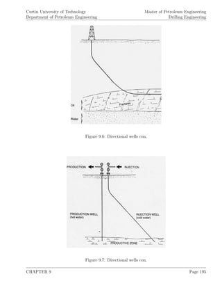
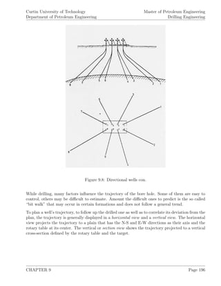
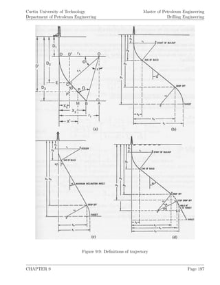
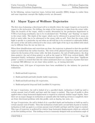
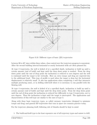
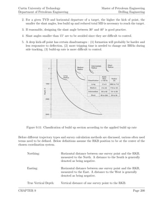
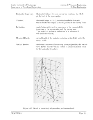
![Curtin University of Technology
Department of Petroleum Engineering
Master of Petroleum Engineering
Drilling Engineering
9.2 Trajectory Calculation
In the following, calculations for the radius of curvature (r1), the maximum inclination angle (θ),
the measured depth and horizontal departure for the buildup intervals as well as the measured
depth and horizontal departure for the holding intervals are presented for different basic trajectory
types.
Build-and-Hold Trajectory
This type of trajectory is most common in the industry whenever applicable. Figure 9.10 shows
this type of trajectory where X3 < r1. TVD and the horizontal departure of the target are denoted
with D3 and X3 respectively, TVD of the kick of point is given by D1. All other parameters are
calculated by the following equations:
Radius of curvature:
r1 =
180
π
.
1
q
(9.1)
where:
q [◦
/ft] ... build up rate or inclination angle buildup
r1 [ft] ... radius of curvature
Maximum inclination angle (θ in [◦
]):
θ = sin−1
r1
(r1 − X3)2
+ (D3 − D1)2
− tan−1 r1 − X3
D3 − D1
(9.2)
Measured depth and horizontal departure along the buildup are computed with:
(DMi
)Build = D1 +
θi
q
(9.3)
(Xi)Build = r1 (1 − cos θi) (9.4)
where, θi = θ at the end of build
θi = sin−1 Di
D1 + r1
(9.5)
CHAPTER 9 Page 202](https://image.slidesharecdn.com/drillingengineering-160119095813/85/Drilling-engineering-210-320.jpg)
![Curtin University of Technology
Department of Petroleum Engineering
Master of Petroleum Engineering
Drilling Engineering
Along the holding interval, the measured depth and horizontal departure are:
(DMi
)Hold = D1 +
θ
q
+
Di − D1 − r1. sin θ
cos θ
(9.6)
(Xi)Hold = r1. (1 − cos θ) + (Di − D1 − r1. sin θ) tan θ (9.7)
where:
Di [ft] ... vertical depth at point i along the buildup or holding interval
Build-Hold-and-Drop (S) Trajectory
The maximum inclination angles can be calculated by following equations:
for r1 + r2 > X4:
θ = tan−1
.
D4 − D1
r1 + r2 − X4
− cos−1 r1 + r2
D4 − D1
. sin tan−1
.
D4 − D1
r1 + r2 − X4
(9.8)
and for r1 + r2 < X4:
θ = 180 − tan−1 D4 − D1
X4 − (r1 + r2)
− cos−1 r1 + r2
D4 − D1
. sin tan−1
.
D4 − D1
X4 − (r1 + r2)
(9.9)
When replacing X4 by X5 + r2.(1 − cos θ ) and D4 by D5 + r2. sin θ , the equations above can be
used to calculate the modified S type trajectory.
9.3 Calculating the Survey of a Well
When drilling a well, inclination, azimuth and MD are measured at various so called “survey
stations”. This is done with survey tools to check the actual traverse of the well. These mea-
surements are then used for (a) estimation of the real trajectory path, (b) comparison with the
planned well trajectory and (c) planning necessary steps to re-direct the well to reach the desired
location.
CHAPTER 9 Page 203](https://image.slidesharecdn.com/drillingengineering-160119095813/85/Drilling-engineering-211-320.jpg)
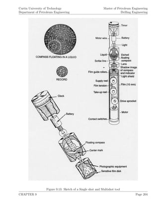
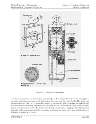
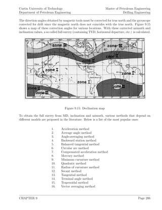
![Curtin University of Technology
Department of Petroleum Engineering
Master of Petroleum Engineering
Drilling Engineering
From the different methods listed above, the minimum curvature and the radius of curvature
methods are considered to be the most accurate ones. The tangential method is the simplest one
to use but gives inaccurate results.
9.3.1 Average angle method
Li = DMi
. sin
αi + αi−1
2
. cos
i − i−1
2
(9.10)
Mi = DMi
. sin
αi + αi−1
2
. sin
i − i−1
2
(9.11)
Di = DMi
. cos
αi + αi−1
2
(9.12)
where:
α [◦
] ... hole angle
[radian] ... azimuth
DMi
[ft] ... measured depth between two survey stations
Li [ft] ... north/south coordinate between the two stations
Mi [ft] ... east/west coordinate between the two stations
The total north/south and east/west coordinates and the TVD value are computed with:
Ln =
n
i=1
Li (9.13)
Mn =
n
i=1
Mi (9.14)
Dn =
n
i=1
Di (9.15)
CHAPTER 9 Page 207](https://image.slidesharecdn.com/drillingengineering-160119095813/85/Drilling-engineering-215-320.jpg)
![Curtin University of Technology
Department of Petroleum Engineering
Master of Petroleum Engineering
Drilling Engineering
9.3.2 Radius of curvature method
Mi =
DMi
2
. [sin αi−1.sin i−1 + sin αi − sin i] .Fi (9.16)
Li =
DMi
2
. [sin αi−1.sin i−1 + sin αi − cos i] .Fi (9.17)
Di =
DMi
2
. [cos αi−1. cos αi] .Fi (9.18)
where:
Fi =
2
βi
[radians] tan
βi
2
[degrees] (9.19)
β = cos−1
{cos [(α2 − α1) − {sin α1. sin α2. [1 − cos ( 2 − 1)]}]} (9.20)
β [radian] ... curvature or the dogleg
F [1] ... ratio factor used to smooth the wellbore between
the two survey stations
α1 [◦
] ... inclination at station 1
α2 [◦
] ... inclination at station 2
1 [◦
] ... azimuth at station 1
2 [◦
] ... azimuth at station 2
When β < 0.25 [radians], F can be set to 1.0
9.3.3 Minimum Curvature Method
Li =
DMi
2
.[sin 1. cos α1 + sin α2. cos 2].RF (9.21)
Mi =
DMi
2
.[sin α1. sin 1 + sin α2. sin 2].RF (9.22)
Di =
DMi
2
.[sin 1 + cos α2. cos 2].RF (9.23)
RF =
360
π.DL
. tan
DL
2
(9.24)
CHAPTER 9 Page 208](https://image.slidesharecdn.com/drillingengineering-160119095813/85/Drilling-engineering-216-320.jpg)
![Curtin University of Technology
Department of Petroleum Engineering
Master of Petroleum Engineering
Drilling Engineering
cos(DL) = cos(α2 − α1) − sin α1. sin α2. (1 − cos( 2 − 1)) (9.25)
where:
DL [◦
/100 ft] ... dog leg
9.4 Dogleg Severity Calculations
By definition, a dogleg is a sudden change of inclination and/or direction of a well’s trajectory.
For description purpose, the change is usually expressed in a 100-[ft] interval ([◦
/ 100 ft]) and
called “dogleg severity”. As it has been seen in practice, large dogleg severities can lead to failure
of drillpipe, drill collar or tool joints as well as create so called “keyseats” which result in stuck
drillstrings.
To obtain the dogleg severity, the survey calculated with one of the methods described above is
used along with following equations:
β = 2. sin−1
. sin2 ∆α
2
+ sin2 ∆
2
. sin2 α + αN
2
(9.26)
or:
β ≈ cos−1
(cos ∆ . sin αN . sin α + cos α. cos αN ) (9.27)
δ =
β
Lc
.100 (9.28)
where:
δ [◦
/100 ft] ... dogleg severity
β [◦
] ... total angle of change (turn)
αN [◦
] ... new inclination
∆ [◦
] ... change in azimuth
∆α [◦
] ... change in inclination
Lc [ft] ... length over which change of trajectory occurs
Note: To reduce the wear-effect of large dogleg severities, the add of multiple steel or rubber
drillpipe protectors which are cylindrical pieces, having an outside diameter equal to the outside
diameter of the tool joints, have proven to be efficient.
CHAPTER 9 Page 209](https://image.slidesharecdn.com/drillingengineering-160119095813/85/Drilling-engineering-217-320.jpg)
![Curtin University of Technology
Department of Petroleum Engineering
Master of Petroleum Engineering
Drilling Engineering
9.5 Deflection Tools and Techniques
The methods presented above calculate the trajectory path of the well as it is drilled. The actual
trajectory is constantly compared with the planned one and in case the actual one is going of course
(which it always does to some extend), correction steps to bring the trajectory on course again have
to be taken. To correct the course of the well in case of minor deflections, an experienced driller can
vary the individual drilling parameters (WOB, RPM, etc.) to adjust for the of-going trajectory.
In case the trajectory is largely of course, a deflection tool has to be run and drilling in sliding
mode (e.g. positive displacement motor (PDM)) carried out to make the necessary correction. To
determine the direction the well is drilled in sliding mode, the bottom hole assembly containing
the deflection tool is rotated from the surface by rotating the whole drill string. Then, either a so
called “Ragland vector diagram” or the following equations are applied to compute the tool face
orientation. The computational results have shown to be more accurate than the graphical one
gained from the Ragland vector diagram. The tool face angle is given by:
γ = cos−1 cos α. cos β − cos βN
sin α. sin β
= sin−1 sin αN . sin ∆
sin β
(9.29)
The new inclination and direction angles are:
αN = cos−1
(cos α. cos β − sin α. sin β. cos γ) (9.30)
∆ = tan−1 tan β. tan γ
sin α + tan β. cos α. cos γ
(9.31)
where for γ is right of high side of the borehole:
N = + ∆ (9.32)
and for γ is left of high side of the borehole:
N = − ∆ (9.33)
where:
N [◦
] ... new direction of the trajectory
αN [◦
] ... new inclination of the trajectory
Although rotary assemblies can be designed to alter the path of the wellbore, there are certain
circumstances where it is necessary to use special deflection tools, for example kicking-off and
CHAPTER 9 Page 210](https://image.slidesharecdn.com/drillingengineering-160119095813/85/Drilling-engineering-218-320.jpg)

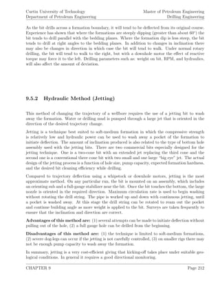
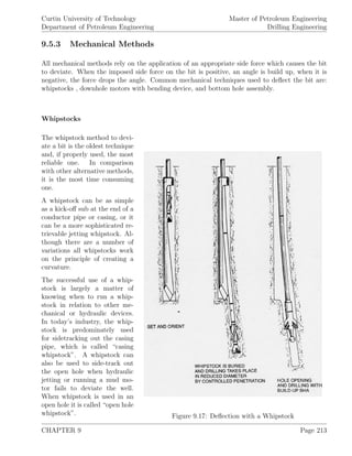
![Curtin University of Technology
Department of Petroleum Engineering
Master of Petroleum Engineering
Drilling Engineering
A whipstock can be described as a steel wedge with a chisel shaped point at the bottom. This
chisel shape prevents the whipstock from turning when drilling begins. The whipstock, that is
run down hole, is attached to the lower end of the drill string by means of a shear pin. It is either
set on the bottom or anchored and locked in a packer which was previously installed in a casing
string.
A modern whipstock has a tapered concave groove, called the tool face, which helps in orienting
the whipstock. Once it is installed down hole, it guides the bit or the mill against the casing or
the open hole wall to drill in the desired direction.
Open Hole Whipstock Running Procedures
The procedures for running the whipstock can be summarized as follows:
1. A whipstock is to be selected according to the wedge needed to effect the desired deflection.
2. A bit that is small enough to fit in the hole with the chosen whipstock is selected.
3. The whipstock is attached to the bottom of the drillstring by means of a shear pin.
4. Having run into the hole, the drillstring is rotated according to the survey information, until
the tool-face of the whipstock is oriented in the desired direction.
5. By applying enough weight, the chisel point is set firmly into the formation or cement plug
to prevent the whipstock from rotating.
6. Additional weight is applied to shear the pin that holds the drill collar to the wedge. Rotation
can then begin.
7. A small diameter pilot hole is drilled to a depth of about 15 [ft] below the toe of the whipstock
at which point the whipstock-stop reaches the top collar of the whipstock.
8. The pilot hole is then surveyed to make sure that it has been drilled in the right direction.
9. After the pilot hole has been surveyed, the bit and the whipstock are tripped out.
10. A hole opener is then run to ream out the pilot hole to the full size hole.
Casing Whipstock Running Procedures
The running steps for a casing whipstock can be summarized as:
1. The casing whipstock packer with anchor device is run to the kick-off point.
2. The alignment key is oriented using a gyro survey, so that the whipstock will land in a
unique position, where the side track is needed.
CHAPTER 9 Page 214](https://image.slidesharecdn.com/drillingengineering-160119095813/85/Drilling-engineering-222-320.jpg)
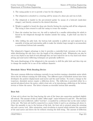
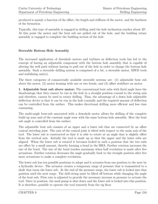
![Curtin University of Technology
Department of Petroleum Engineering
Master of Petroleum Engineering
Drilling Engineering
The greater the stabilizer offset (higher under-gauge blade), the greater the rate of build, but the
amount of offset is limited.
Once the wellbore is brought back onto the planned trajectory, the drillstring can be rotated.
Rotating the offset stabilizer results in a slightly over-gauge hole.
9.6 While Drilling Techniques
With “while drilling techniques”, the direction of the wellbore, condition of the drillstring as well
as the formations that have been penetrated can be measured and the measurements transferred
to the rig-site while drilling. While drilling sensors are typically mounted at the BHA as close
as possible to the bit. Depending on the drillstring configuration, the distance between the bit
and the measuring devices can be as little as 10 [ft]. In this way, the measurements taken are
somewhat behind the bit and depending on the penetration rate, are recorded with some lag-time.
While drilling systems generally consist of (a) a power system, (b) measuring sensors and (c) a
telemetry system for data transfer. The power system can be either based on a battery, a turbine
or a combination of them. Batteries have the advantage that no circulation is needed to carry out
measurements, thus while tripping, control logs can be run.
9.6.1 Measurement While Drilling
The term “measurement while drilling” (MWD) refers to the while drilling measurement of di-
rectional parameters (MD, inclination, azimuth) as well as certain drilling parameters like WOB,
downhole torque, temperature, etc. The sensor to perform these measurements are three orthogo-
nal fluxgate magnetometers and three accelerometers. The use of gyroscope navigated MWD offers
significant benefits over navigation sensors. They offer greater accuracy and are not susceptible
to inference from magnetic fields.
The drilling parameters measured with MWD tools are aimed to increase the drilling efficiency
(stick-slip), be applied to detect abnormal formation pressures or any kind of hole problems.
Most MWD tools can operate at tool-temperatures up to 150 ◦
C, some sensor work up to 175 ◦
C.
It should be noted that the tool-temperatures are generally about 20 ◦
C less than the formation
temperatures, measured by wireline logs which is caused by the cooling effect of mud circulation.
Downhole pressures create less problems for MWD tools than downhole temperatures. Most MWD
tools are designed to withstand up to 20,000 [psi] which is rarely encountered.
MWD tools are most sensitive to shock and vibrations. Torsional shock, created by stick-slip have
been found to be able to cause tool failure, lateral shocks which can be magnitudes higher than
axial shocks, can be reduced by the use of jars.
Normally sensors measure MWD shock loads constantly and transmit them to the rick. There the
driller can manipulate the drilling parameters to keep them in acceptable limits.
CHAPTER 9 Page 218](https://image.slidesharecdn.com/drillingengineering-160119095813/85/Drilling-engineering-226-320.jpg)
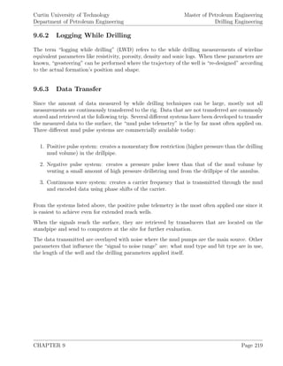
![Curtin University of Technology
Department of Petroleum Engineering
Master of Petroleum Engineering
Drilling Engineering
9.7 Examples
1. Calculate a build-and-hold trajectory to reach a target at 10,000 [ft] TVD and 2,600 [ft]
horizontal departure. The kick off point shall be set to 1,500 [ft] and a build rate of 2 [◦
/ 100
ft] applied. Compute the: radius of curvature, maximum inclination angle, measured depth and
horizontal departure at the end of build as well as the measured depth and horizontal departure
at 8,000 [ft].
2. When the inclination has changed from 5◦
to 7◦
together with a change of direction from N90E
to S82E over an interval of 75 [ft], what is the dogleg severity?
3. After going of course the trajectory has to be changed in inclination from 4◦
to 6◦
as well as
in direction from 15◦
to 35◦
over the next 70 [ft], what is the tool-face setting and the expected
dogleg severity?
CHAPTER 9 Page 220](https://image.slidesharecdn.com/drillingengineering-160119095813/85/Drilling-engineering-228-320.jpg)
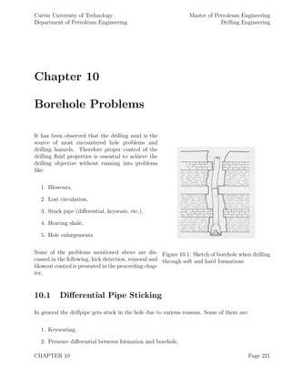
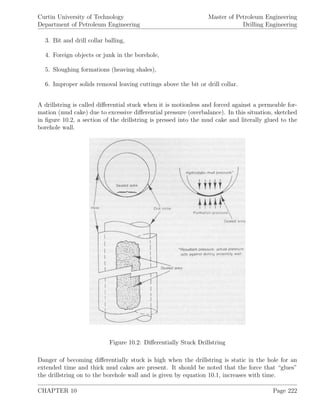
![Curtin University of Technology
Department of Petroleum Engineering
Master of Petroleum Engineering
Drilling Engineering
Fst = 12.hf .tmc. (ph − pf ) .f (10.1)
When the borehole is in-gauge, the term A = hf .tmc is expressed by:
A = 2.hf .
d2
2
− tmc
2
−
d2
2
− tmc.
d2 − tmc
d2 − d1
2
(10.2)
for
tmc ≤
d1
2
≤
d2 − tmc
2
(10.3)
where:
Fst [lbf] ... force necessary to free pipe
hf [ft] ... formation thickness
tcm [in] ... thickness of mud cake
ph [psi] ... hydrostatic pressure in the borehole
pf [psi] ... formation pressure
f [1] ... friction factor, function of time,
d1 [in] ... outer diameter of the drillstring where it is stuck
d2 [in] ... borehole diameter where pipe is stuck
12 [in/ft] ... conversion factor [in] -> [ft]
The friction factor f depends on the composition of the mud cake, variation of the contact between
drillstring and mud cake and the time since the drillstring got stuck. The value of the friction
factor ranges from 0.2 to 0.6.
To minimize the danger of getting differentially stuck, following precautions should be applied:
1. Minimize the differential pressure (overbalance) between borehole pressure and formation
pressure,
2. Maintain efficient control of the mud properties,
3. Minimize the contact area between drillstring and borehole,
4. Minimize the non-rotating time of the drillstring,
5. Minimize the friction factor.
The contact area between the drillstring and the borehole can be minimized by:
CHAPTER 10 Page 223](https://image.slidesharecdn.com/drillingengineering-160119095813/85/Drilling-engineering-231-320.jpg)
![Curtin University of Technology
Department of Petroleum Engineering
Master of Petroleum Engineering
Drilling Engineering
1. Using stabilizers on the drill collars,
2. Using grooved or noncircular drill collars,
3. Using drill collars with external upset,
4. Minimize filter cake thickness through proper design of the drilling mud.
The friction factor can be minimized by using low water-loss muds, oil-base muds and walnut
hulls.
10.2 Free Point Calculation
In order to take actions to free the pipe, the knowledge of the depth where the drillstring is stuck,
also called “free point”, is vital. Two methods are available to verify the free point location:
(a) measurement of the drillstring stretch, measured at the surface when the string is pull with a
certain amount of overpull and, (b) usage of so called “free point indicators”. Free point indicators,
which are either strain gauge probes or subsurface probes, are special gauge tools that measure
the strain in the drillstring.
To compute the free point based on the drillpipe stretch, only measurements taken at the derrick
are required. The procedure is summarized as:
1. Pulling the drillstring with normal hook load and mark a reference point X1 on the pipe.
2. Pull the drillstring with additional 20,000 to 40,000 [lbf], a force F that causes a stretch of
the free portion of the drillstring. At the reference point-level, mark the drill pipe for X2.
The stretch in [in] is given by X2 −X1. Note that the applied overpull force must not exceed
the yield strength of the pipe or the joints.
3. Use equation 10.4 to compute the free point location:
Lst =
735, 294. (X2 − X1) .Wdp
F
(10.4)
where:
Lst [ft] ... length of free portion of the pipe, depth of free point
Wdp [lb/ft] ... nominal weight of drillpipe
F [lbf] ... additional force (overpull)
As it can be seen, equation 10.4 accounts for the stretch of the drillpipe only.
CHAPTER 10 Page 224](https://image.slidesharecdn.com/drillingengineering-160119095813/85/Drilling-engineering-232-320.jpg)
![Curtin University of Technology
Department of Petroleum Engineering
Master of Petroleum Engineering
Drilling Engineering
10.3 Freeing Differentially Stuck Pipe
When the location of the free point is verified, following methods to free the drillstring are possible
and should be tried in the order they are listed below.
10.3.1 Spotting Organic Fluids
A mixture of diesel and surfactants is pumped to the location where the drillstring is stuck. This
is performed by pumping the mixture through the drillstring and up the annulus to the free point
depth. Since the mixture is meant to reduce the thickness of the mud cake and the friction factor,
sufficient time has to be allowed so that the mixture can be dissolved and the mud cake destroyed.
While spotting, the drillstring is worked continuously to free the drillstring.
10.3.2 Hydrostatic Pressure Reduction
This method aims to create a pressure differential between the inside of the drillpipe and the
annulus by pumping lower density fluid into the drillpipe. Since the hydrostatic pressure from
the fluid inside the drillpipe and from the annulus have to be the same at the bottom of the hole,
the mud level at the annulus as well as the pressure at the free point are reduced. The amount
of low density fluid to be pumped into the drillstring and the resulting maximum drillpipe gauge
pressures are given by:
Vo =
Lst.Vdp
ρm − ρo
. ρm −
pp
0.052.Lst
. 1 +
Van
Vdp
. 1 −
ρo
ρm
(10.5)
(pdp)max = 0.052.
Vo
Vdp
. (ρm − ρo) (10.6)
The fluid level drop in the annulus [ft] can be computed with:
∆FL = Lst −
pp
0.052.ρm
(10.7)
The equivalent mud weight during this bleed-off procedure is found as:
ρe = ρm −
(pdp)max − pdp
0.052.Lst. 1 + Van
Vdp
. 1 − ρo
ρm
(10.8)
where:
Vdp [bbl/ft] ... capacity of drillpipe
CHAPTER 10 Page 225](https://image.slidesharecdn.com/drillingengineering-160119095813/85/Drilling-engineering-233-320.jpg)
![Curtin University of Technology
Department of Petroleum Engineering
Master of Petroleum Engineering
Drilling Engineering
Van [bbl/ft] ... capacity of annulus
pp [psi] ... pore pressure
pdp [psi] ... pressure within the drillpipe,
measured at the surface
(pdp)max [psi] ... maximum drillpipe pressure
ρm [ppg] ... mud density
ρo [ppg] ... density of fluid pumped down
Vo [bbl] ... volume of the fluid pumped down
Lst [ft] ... length of the drillstring
D [ft] ... total depth of the well (MD)
It should be noted that precautions have to be taken that formations above the free point do not
kick due to the pressure reduction of the annulus.
As alternative procedure to the method described above, the low density fluid can be pumped
into both, the drillpipe and the annulus. Here the volumes of low density fluid required to reduce
the differential pressure Vo and the volume of mud Vm required to pump behind the low density
fluid are determined by:
Vo = Van.
pp
0.052
− Lst.ρm
ρo − ρm
(10.9)
Vm = Vdp.Lst + Van. (D − Lst) (10.10)
10.3.3 Backoff Operations
When all attempts to free the stuck drillstring failed, backoff operations are the last alternative.
By backoff operations parting the drillstring above the free point, recovering the free part of the
drillstring and fishing the remaining, stuck part of the string are understood.
Parting of the Drillstring
Nowadays four different methods are applied to part the drillstring:
1. Unscrew the pipe at a selective threaded joint above the stuck point using a prima cord
explosive run on a electric wireline.
2. Chemical cut - An electrical wireline tool and procedure that uses a propellant and a chem-
ical, halogen fluoride, to burn a series of holes in the pipe thereby weakening it so that it
easily pulls apart with a slight pull.
CHAPTER 10 Page 226](https://image.slidesharecdn.com/drillingengineering-160119095813/85/Drilling-engineering-234-320.jpg)
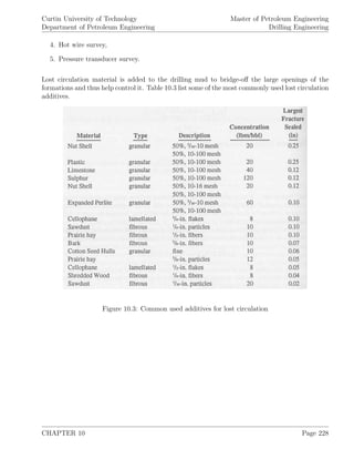
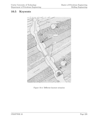
![Curtin University of Technology
Department of Petroleum Engineering
Master of Petroleum Engineering
Drilling Engineering
10.6 Examples
1. In a 9,500 [ft] hole the drillstring is stuck at 8,000 [ft]. What is the volume of oil required
to pump through the drillstring to free the pipe when the pore pressure is estimated to be 4,300
[psi] at the stuck depth. Following further well data are available: ρm = 12 [ppg], ρo = 8 [ppg],
Vdp = 0.0178 [bbl/ft], Van = 0.0544 [bbl/ft].
2. Determine the density, length and type of kick using the following information: Vk = 20 [bbl],
Ldc = 900 [ft], ρm = 9.6 [ppg], d2 = 9.875 [in], d1c = 7.785 [in], dip = 4.2 [in], pc = 720 [psi],
pdp = 520 [psi].
3. When drilling a 8-1
2
[in] hole, a kick is taken at 9,500 [ft]. After shutting in, the stabilized
drillpipe pressure and the casing shut-in pressure are found to be 300 [psi] and 600 [psi] respectively.
The recorded pit gain is 20 [bbl], pre-kick information contain: dh = 8.5 [in], ddc = 3.0 [in],
ddp = 4.276 [in], Ldc = 600 [ft], Ddc = 8 [in], Ddp = 5 [in], ρm = 11 [ppg], (pp)str=60 = 2, 000 [psi],
(pp)str=30 = 500 [psi]. Applying the wait-and-weight method, compute the:
(a) Bottom hole pressure,
(b) Kill mud weight,
(c) Standpipe pressure at start of circulation of
heavier mud,
(d) Final circulation pressure,
(e) Time required to replace the contents of the drillstring
with the kill mud,
(f) Total time required to replace the contents of the
well with kill mud,
(g) Total number of strokes required assuming that the
pump factor is 0.15 [bbl/stroke],
(h) Maximum casing pressure when the kick reaches the surface,
(i) Expected pit gain as the top of the kick reaches the surface.
CHAPTER 10 Page 230](https://image.slidesharecdn.com/drillingengineering-160119095813/85/Drilling-engineering-238-320.jpg)
![Curtin University of Technology
Department of Petroleum Engineering
Master of Petroleum Engineering
Drilling Engineering
1. Gain in pit volume,
2. Increase in mud return flow rate while circulating at constant rate,
3. Mud return even when the pumps are shut down,
4. Well is taking less (tripping in) or giving more (tripping out) mud than calculated,
5. Increase in drilling rate,
6. Decrease in the circulation pressure,
7. Increase of the chloride content of the mud,
8. Increase of trip, connection or background gas.
It should be noted that some of these parameters alone are sufficient to indicate a kick (e.g. pit
gain), others (e.g. reduction of chloride content) are additional observations and should only be
used as kick detection when multiple other kick detecting observations are present as well. Small
trip tanks have proven to provide the best means of monitoring hole fill-up volume. Trip tanks
usually hold 10 to 15 [bbl] and have 1 [bbl] gauge markers. On the site, the top of the gravity-feed
trip tank must be slightly lower than the bell nipple to prevent mud from being lost to the flow
line. In case that a trip tank is not installed, hole fill-up volume should be determined by counting
pump strokes each time the hole is filled.
11.1 Blowout Preventer
When a kick is detected at the surface, a device called “blowout preventers” (BOP) is used to stop
the fluid flow from the well. To cover all possible scenarios and handle different kick situations,
different BOPs are collectively attached to the well head. This series of BOPs is also called “BOP
stack”. A typical BOP stack configuration is shown in figure 11.1.
The BOP stack should enable the rig personnel to perform following actions when a kick is shut
in:
1. BOP must be capable to terminate flow from the well under all drilling conditions.
2. When the drillstring is in the hole, movement of the string without releasing well pressure
must be possible.
3. BOP stack must allow fluid circulation through the well annulus under pressure.
To achieve these objectives, a series of so called “ram preventers” and “annular preventers” are
combined.
CHAPTER 11 Page 232](https://image.slidesharecdn.com/drillingengineering-160119095813/85/Drilling-engineering-240-320.jpg)
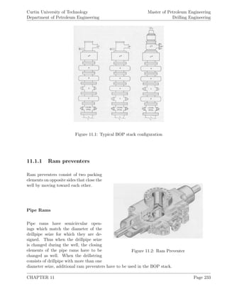
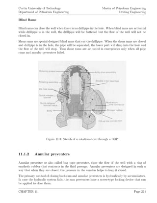
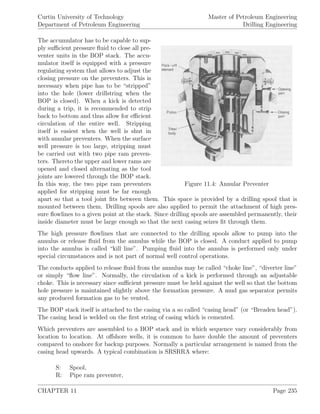
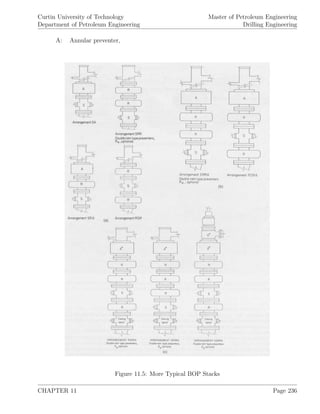
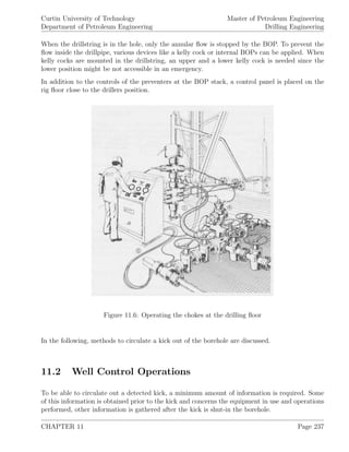
![Curtin University of Technology
Department of Petroleum Engineering
Master of Petroleum Engineering
Drilling Engineering
Pre-kick information:
1. Maximum allowable casing pressure (pressure rating of the BOP and burst strength of the
casing),
2. Capacity [bbl/ft] of the drillpipe, the drill collars, and annuli,
3. Volume of active mud circulation system,
4. Fracture gradient of the drilled formation,
5. Reduced circulation rate and pressure,
6. Pump factor and efficiency.
After a kick is detected and the well shut-in, the following parameters are obtained:
Post-kick information:
1. Stabilized shut-in casing pressure,
2. Stabilized shut-in drillpipe pressure,
3. Pit gain (is assumed to be equal the kick volume),
4. TVD and MD depth of the bottom of the hole.
Figure 11.7: Shutting in a kick
CHAPTER 11 Page 238](https://image.slidesharecdn.com/drillingengineering-160119095813/85/Drilling-engineering-246-320.jpg)
![Curtin University of Technology
Department of Petroleum Engineering
Master of Petroleum Engineering
Drilling Engineering
Having all the information at hand, following parameters are determined before attempting to
circulate out the kick:
1. Density (determines type) and length of kick,
2. Mud weight required to stop well from kicking,
3. Number of pump strokes to pump a volume from surface to bit and from bit to choke,
4. Volume of weighted mud to kill well,
5. Quantity of weighting material (e.g. barite) required to weight up the drilling fluid,
6. Accurate initial circulation drillpipe pressure,
7. Accurate final circulation drillpipe pressure,
8. Drillpipe pressure reduction schedule (for wait-and-weight method).
11.3 Length and Density of Kick
To determine the type of kick taken (oil, water, gas), the density of the gained fluid (kick density)
has to be estimated. This is achieved by combining the observed drillpipe pdp and the casing
pressure pc as well as the gain in pit volume. Equation 11.1 calculates the kick density [ppg]:
ρk = ρm −
pc − pdp
0.052.Lk
(11.1)
To solve this equation, the kick length Lk [ft], which is estimated by the pit gain and the geomet-
rical configuration of the drillstring and the diameter of the borehole, has to be computed first.
For a pit gain Vk smaller or equal the annulus volume of the drill collars (Van)dc, the length of the
kick is found by equation 11.2:
Lk = Vk. (Van)dc (11.2)
For a pit gain Vk larger than the annulus volume of the drill collars (Van)dc equation 11.3 has to
be used.
Lk = Ldc + Vk −
Ldc
(Van)dc
. (Van)dp (11.3)
where:
CHAPTER 11 Page 239](https://image.slidesharecdn.com/drillingengineering-160119095813/85/Drilling-engineering-247-320.jpg)
![Curtin University of Technology
Department of Petroleum Engineering
Master of Petroleum Engineering
Drilling Engineering
(Van)cd [ft/bbl] ... annular capacity of the borehole at the drill collars
Ldc [ft] ... total length of the drill collars
(Van)dp [ft/bbl] ... annular capacity of the borehole at the drillpipe
Vk [bbl] ... kick volume, pit gain
Pc [psi] ... initial stabilized casing pressure
Pdp [psi] ... initial stabilized drillpipe pressure
Knowing the kick density, the so called kick gradient gradk [psi/ft] is often applied to identify the
type of kick. The kick gradient is computed as:
gradk = 0.052.ρk (11.4)
where:
ρk [ppg] ... kick density
Thus:
gradk < 0.3 ... gas kick
0.3 < gradk < 0.4 ... oil and gas mixture
gradk > 0.4 ... water kick
gradk > 8.33 ... salt water kick
11.4 Kick Tolerance and Kill Mud Weight
The kick tolerance determines the ability to control a kick at the current situation without frac-
turing a formation and causing lost circulation.
By definition, the kick tolerance is the difference between the maximum pore pressure of any
formation penetrated and causing the kick, and the drilling mud weight at this depth. This is
mathematically expressed as:
Tk = (ρe − ρm) (11.5)
To establish safe drilling condition, it should be ensured that the kick tolerance is never below 1
[ppg]. The kill mud weight is defined as the mud weight required to stop a well from kicking and
can be computed by:
CHAPTER 11 Page 240](https://image.slidesharecdn.com/drillingengineering-160119095813/85/Drilling-engineering-248-320.jpg)
![Curtin University of Technology
Department of Petroleum Engineering
Master of Petroleum Engineering
Drilling Engineering
ρkm = ρm +
pdp
0.052.D
(11.6)
The equivalent mud density at the casing seat is found as:
ρe =
pc
0.052.Dc
+ ρm (11.7)
where:
Dc [ft] ... casing setting depth
11.5 Pump Pressure Schedules for Well Control Opera-
tions
When killing a well, the bottom hole pressure of the well must be maintained equal to or higher
than the formation pressure which caused the kick. When this is not established, the well would
be constantly kicking, thus constantly gaining formation fluid or gas.
To maintain this required bottom hole pressure, the circulation pressure to remove the kick has
to be calculated as planned pump rate for kick removal. Normally, the pump rate to circulate
out a kick is half the drilling pump rate. It is common practice to calculate the required circu-
lation pressure since the required bottom hole pressure is not directly measurable. The required
circulation pressure can be found as:
pdpff = pdp + ∆pp − ∆pdpf = pdpf − ∆pdpf (11.8)
where:
∆pdpf = (ρkm − ρm) . 0.052.D −
∆pp
ρm
(11.9)
This enables the calculation of the total number of pump strokes required to pump the kill mud
to the bit:
fstr =
Ldp.Vdp + Ldc.Vdc
Fp
(11.10)
where:
CHAPTER 11 Page 241](https://image.slidesharecdn.com/drillingengineering-160119095813/85/Drilling-engineering-249-320.jpg)
![Curtin University of Technology
Department of Petroleum Engineering
Master of Petroleum Engineering
Drilling Engineering
pdpff [psi] ... final circulation drillpipe pressure
∆pdpf [psi] ... change in total drillpipe pressure required
to maintain the bottom hole pressure constant
∆pp [psi] ... routinely measured circulation pump pressure
Fp [bbl/stroke] ... pump factor
Ldp [ft] ... length of drillpipe
Ldc [ft] ... length of drill collars
Vdp [bbl/ft] ... capacity of drillpipe
Vdc [bbl/ft] ... capacity of drill collar
The number of strokes pumped and the circulation drillpipe pressure are linearly related. This
can be seen with equation 11.11:
dpn = pdpf −
pdpf − pdpff
fstr
.Str (11.11)
where:
Str [# strokes] ... intermediate pump strokes
11.6 Kick Removal – Two Methods
In general, two methods to circulate a kick out are applied most often:
1. Driller’s method,
2. Wait-and-weight method.
At the wait-and-weight method, the well is closed-in once a kick is detected and the post-kick
information is obtained. Next, the kill mud weight is determined, the weighted mud is prepared
and then circulated in to kill the well. During this operation, the drillpipe pressure is checked
according to the pressure schedule which has to be prepared before the circulation starts.
When the driller’s method is applied to kill the well, the whole process is divided into two steps.
First, the annulus fluid containing the kick is displaced with the help of an adjustable choke.
Normally, circulation is continued so that all kick fluids are removed. Then, as a second step, the
weighted mud is pumped through the drillstring and the annulus by a complete circulation.
The driller’s methods offers following advantages compared to the weight-and-weight method:
1. Circulation starts immediately,
CHAPTER 11 Page 242](https://image.slidesharecdn.com/drillingengineering-160119095813/85/Drilling-engineering-250-320.jpg)
![Curtin University of Technology
Department of Petroleum Engineering
Master of Petroleum Engineering
Drilling Engineering
2. Sufficient time is given to weighting up the mud.
The disadvantages of the driller’s method compared to the wait-and-weight method are:
1. Maximum surface pressure and pressure at the casing shoe are higher,
2. Surface equipment is subjected to higher pressures for a longer time.
11.6.1 Wait-and-weight method
pbh = pdp + 0.052.ρm.D (11.12)
G =
Vk.pbh
pmax
(11.13)
pmax =
√
b2 + 4.c + b
2
(11.14)
b =
pdp.Vdp. (Van)dp
D
+ 0.052.ρkm.D1 (11.15)
c = 0.052.ρkm.Vk. (Van)dp .pbh (11.16)
where:
pbh [psi] ... bottom hole pressure
G [bbl] ... pit volume increase when top of kick reaches the depth of interest
pmax [psi] ... maximum casing pressure
Vdp [bbl] ... inside drillpipe capacity
(Van)dp [ft/bbl] ... annular capacity opposite the drillpipe
D1 [ft] ... depth to the point where kick severity calculation is required
ρm [ppg] ... kill mud weight
D [ft] ... total depth of the well
CHAPTER 11 Page 243](https://image.slidesharecdn.com/drillingengineering-160119095813/85/Drilling-engineering-251-320.jpg)
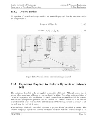
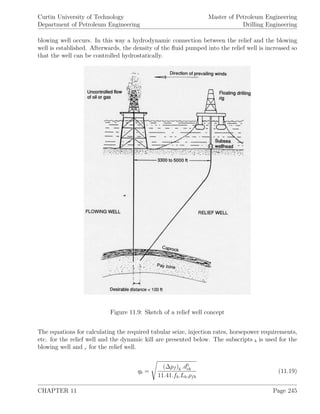
![Curtin University of Technology
Department of Petroleum Engineering
Master of Petroleum Engineering
Drilling Engineering
d5
eb = (dob − dib)3
. (dob − dib)2
(11.20)
fb =
0.25
2. log dh
+ 1.14
2 (11.21)
(∆pf )b = pb − phb (11.22)
qr =
qb
ηe
(11.23)
hp = 0.0245.qr.psr (11.24)
The minimum tubular seize of the relief well:
d5
er
fr
>
11.41.q2
r .Lr.ρfr
(∆pf )r
(11.25)
d5
er = (dor − dir)3
. (dor − dir)2
(11.26)
(∆pf )r = psr + phr − pfrac (11.27)
(pmax)b =
Wsb + (Aan)b .R.phb
(Ap)b + (Aan)b
(11.28)
R =
1
2. ln dob
dib
−
d2
ib
d2
ob − d2
ib
(11.29)
qmax = −
(pfrac − pb) .k.h
101, 664.β.µ. ln 1,688.φ.µ.ct.r2
w
k.t
− 2.s
(11.30)
qb [bbl/min] ... flow rate needed in the blowout well
qr [bbl/min] ... injection rate needed in the relief well
hp [hp] ... pumping power requirement
(pmax)b [psi] ... maximum allowable bottom hole pressure
Aan [in2
] ... area of annulus
Ap [in2
] ... area of drillpipe
ct [1/psi] ... total isothermal compressibility
CHAPTER 11 Page 246](https://image.slidesharecdn.com/drillingengineering-160119095813/85/Drilling-engineering-254-320.jpg)
![Curtin University of Technology
Department of Petroleum Engineering
Master of Petroleum Engineering
Drilling Engineering
d [in] ... hole or casing inside diameter
de [in] ... equivalent pipe diameter
dh [in] ... hydraulic diameter (= (do − di))
di [in] ... outside diameter of the inside pipe
do [in] ... inside diameter of the outside pipe
f [1] ... friction factor
h [ft] ... net pay thickness
k [md] ... formation permeability
L [ft] ... length of pipe
p [psi] ... required bottom hole pressure
pf [psi] ... required friction pressure drop
pfrac [psi] ... fracture pressure of formation
ph [psi] ... hydrostatic head of fluids
ps [psi] ... maximum allowable surface injection pressure
pmax [psi] ... maximum allowable bottom hole pressure
∆pf [psi] ... maximum allowable friction pressure drop
q [bbl/min] ... frow rate or injection rate
qmax [bbl/min] ... maximum allowable injection rate through formation
R [1] ... ratio of friction drag on drillstring to total fraction
rw [ft] ... wellbore radius in relief well
s [1] ... skin factor of relief well
t [min] ... pumping time
Ws [lb] ... weight of drillstring in air
ρf [ppg] ... density of kill fluid
µ [cp] ... viscosity of injected fluids
φ [%] ... formation porosity
β [RB/STB] ... formation volume factor of injected fluids
[in] ... ripe roughness factor, 0.00065
ηe [%] ... efficiency
Normally, relief well killing operations are carried out by companies specialized in killing blowouts.
The same is valid for a surface kill of a blowout.
CHAPTER 11 Page 247](https://image.slidesharecdn.com/drillingengineering-160119095813/85/Drilling-engineering-255-320.jpg)

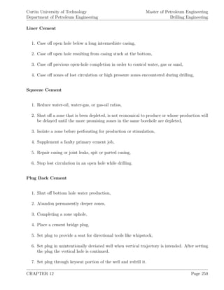
![Curtin University of Technology
Department of Petroleum Engineering
Master of Petroleum Engineering
Drilling Engineering
12.2 Properties of Cement Slurry
API has defined standard classes (Class A to Class H) as well as standard types of cement used
within oil and gas wells. The standard types are:
1. Ordinary,
2. Moderate sulfate-resistant,
3. High sulfate-resistant,
the standard classes are defined as:
1. Class A: Intended depth range for usage: surface to 6,000 [ft], when special properties are
not required, available in ordinary type only.
2. Class B: Intended depth range for usage: surface to 6,000 [ft], when conditions require
moderate to high sulfate-resistance, available as moderate and high sulfate-resistance types.
3. Class C: Intended depth range for usage: surface to 6,000 [ft], when condition require high
early strength, available in ordinary, moderate and high sulfate-resistance types.
4. Class D: Intended depth range for usage: 6,000 to 10,000 [ft], at moderately high temper-
atures and pressures conditions, available in moderate and high sulfate-resistance types.
5. Class E: Intended depth range for usage: 10,000 to 14,000 [ft], at high temperature and
pressure conditions, available in moderate and high sulfate-resistance types.
6. Class F: Intended depth range for usage: 10,000 to 16,000 [ft], at extremely high tempera-
ture and pressure conditions, available in moderate and high sulfate-resistance types.
7. Class G: Intended as basic cement in the depth range: surface to 8,000 [ft], when used
with accelerators and retarders covers wide range of temperatures and pressures, no other
additions than calcium sulfate, water or both are to be blended with the clinker, available
in moderate and high sulfate-resistance types.
8. Class H: Intended as basic cement in the depth range: surface to 8,000 [ft], when used
with accelerators and retarders covers wide range of temperatures and pressures, no other
additions than calcium sulfate, water or both are to be blended with the clinker, available
in moderate sulfate-resistance type only.
Cement properties include the chemical, physical and rheological characteristics of the cement.
The rheological properties of cement slurries are generally the same as the ones of the drilling
fluids discussed in previous sections. The chemical properties and requirements of API cement
types are given in table 12.1, some physical properties are provided in table 12.2 as well.
CHAPTER 12 Page 251](https://image.slidesharecdn.com/drillingengineering-160119095813/85/Drilling-engineering-259-320.jpg)
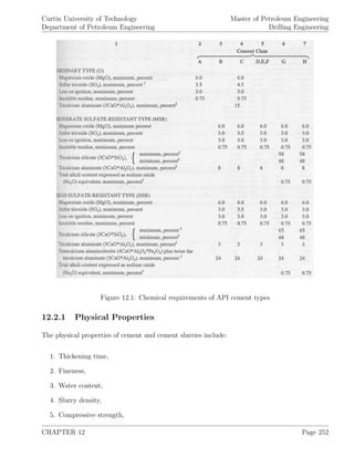
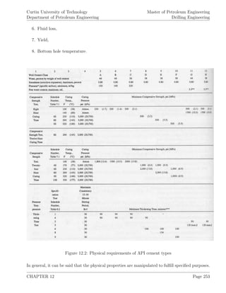
![Curtin University of Technology
Department of Petroleum Engineering
Master of Petroleum Engineering
Drilling Engineering
Slurry density
To minimize the danger of fracturing the formations, lost circulation or kicks, the cement slurry
density should be the same as the drilling fluid density at cementing operations. The following
equation gives the slurry density ρcs in [ppg]:
ρcs =
[lb] Cement + [lb] Water + [lb] Additive
[gal] Cement + [gal] Water + [gal] Additive
(12.1)
To compute the absolute volume of solid constituents, the equation 12.2 is applied:
gal =
lb of Material
(8.34 ppg)(s.g. of Material)
(12.2)
Yield
By definition, the yield is the volume of cement slurry obtained when mixing one sack of cement
with a specified amount of water as well as other additives. Note that one sack cement (94 [lb]
sack) contains 1 [ft3
] bulk volume and 0.48 [ft3
] absolute volume. To compute the yield in [ft3
],
equation 12.3 is applied:
Yield =
[gal] Cement + [gal] Water + [gal] Additive
7.48 gal
ft3
(12.3)
Thickening Time
The length of time the cement slurry is pumpable is also called “thickening time”. To control the
thickening time, adding of setting time retarders, a reduction of rapidly hydrating components and
an adjustment of the cement fineness is performed. When the time it takes to properly place the
cement slurry at the predetermined annulus interval (mixing and displacement time), including a
safety factor, exceeds the thickening time, parts of the cement will remain in the tubular used to
pump down the cement slurry. To determine the mixing and displacement times, equations 12.4
and 12.5 applied:
Tm =
Volume of Dry Cement
Mixing Rate
(12.4)
Td =
Amount of Fluid Required to Displace Top Plug
Displacement Rate
(12.5)
CHAPTER 12 Page 254](https://image.slidesharecdn.com/drillingengineering-160119095813/85/Drilling-engineering-262-320.jpg)
![Curtin University of Technology
Department of Petroleum Engineering
Master of Petroleum Engineering
Drilling Engineering
Compressive Strength
To hold the casing in place, enable support capability of the surface wellhead equipment and with-
stand the differential pressures across the cement-formation interface, the compressive strength of
the set and hardened cement has to be high enough. As general practice, 500 [psi] of compres-
sive strength has to be developed by the hardening cement before any other downhole operation
commences. The time it takes the cement to reach this minimum compressive strength is often
referenced as “wait on cement” (WOC). During this time, other routine surface service operations
are usually carried out. The support capability of the cement is given by:
F = 0.969.Sc.do.H (12.6)
where:
F [lbf] ... support capability
Sc [psi] ... compressive strength of cement
do [in] ... outside diameter of casing
H [ft] ... hight of cement column
12.3 Cement Additives
Main component of all cement slurries for oil and gas well cementing is “Portland cement”. It is
produced according to API specifications by taking raw material like limestone, clay or shale, and
iron ore. After mixing and grinding, they are fed into a kiln where they are melt into a substance
called “cement clinker”. This clinker is then ground into a powdery mixture and combined with
small amounts of gypsum or other components.
To better fit the individual well requirements, the properties of the cement slurry and hardened
cement have to be adjusted. Therefore, certain cement additives are mixed into the slurry. The
additives can be grouped according to their functionality into:
1. Extenders,
2. Accelerators,
3. Retarders,
4. Weighting material,
5. Fluid loss or filtration control material,
6. Dispersants or thinners.
CHAPTER 12 Page 255](https://image.slidesharecdn.com/drillingengineering-160119095813/85/Drilling-engineering-263-320.jpg)
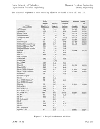
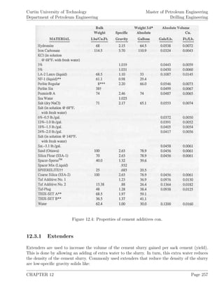
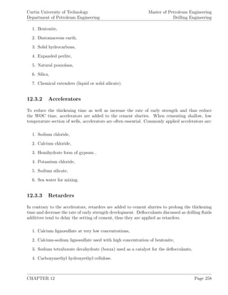
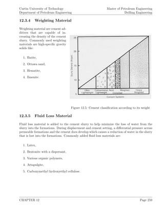
![Curtin University of Technology
Department of Petroleum Engineering
Master of Petroleum Engineering
Drilling Engineering
12.3.6 Dispersants
Figure 12.6: Water requirements for mixing ce-
ment slurries
Dispersants are added to thin the cement
slurry. This causes a reduction of slurry vis-
cosity and is achieved without adding of extra
water. Commonly applied thinners are:
1. Calcium lignosulfate,
2. Sodium chloride,
3. Certain long chain polymers.
The water requirement of mixing API cement
and some additives are shown in table 12.6.
To obtain the required density of the cement
slurry by adding high-specific gravity material
(per 94 [lb] sack of cement), the equation 12.7
can be applied:
Madditive =
94.ρcs2
8.34.γc
+ ρcs2.Vwc − 94
8.34.Vwa
100
+ 1 − ρcs2
8.34.γa
− ρcs2.Vwa
100
(12.7)
When blending materials with saltwater, ideal
mixing rules do not apply. Therefore to cal-
culate the yield weight of bentonite, the water
requirements and the weight of NaCl or CaCl2
to obtain a specific concentration of chlorides
and bentonite, following equations have to be
applied:
Sacks of Cement =
Vcs
Yield
(12.8)
MB =
% Bentonite
100
.94. (Sacks of Cement)
(12.9)
Vw =
W
C
. (Sacks of Cement)
42
(12.10)
CHAPTER 12 Page 260](https://image.slidesharecdn.com/drillingengineering-160119095813/85/Drilling-engineering-268-320.jpg)
![Curtin University of Technology
Department of Petroleum Engineering
Master of Petroleum Engineering
Drilling Engineering
MChlorides =
% Chlorides
100
.94. (Sacks of Cement) (12.11)
% Chloride/Wt. of Water =
94. (% Chloride)
8.34.W
C
+ 94. (% Chloride/100)
(12.12)
Yield = 0.47975 + 0.56846.
% Bentonite
100
+
94. (% Chloride/100) + 8.34.W
C
62.4.γChlorides
(12.13)
where:
Vwa [gal/sack] ... water requirement for additive
Vwc [gal/sack] ... water requirement for cement
γa [s.g.] ... specific gravity of additive
γc [s.g.] ... specific gravity of cement
ρcs2 [ppg] ... density of weighted slurry
Madditive [lb/sack] ... weight of additive required to raise the density to ρcs2
Vcs [ft3
] ... slurry volume
W
C
[gal/sack] ... water/cement ratio
γchlorides [s.g.] ... specific gravity of salt water as per percent chlorides
MB [lb] ... weight of bentonite to be added
Mchlorides [lb] ... weight of chlorides to be added
yield [ft3
/sack]
% Cloride is the % NaCl or % CaCl2 by weight of cement
% Bentonite ie % bentonite by weight of cement
Specific gravities with respect to various concentrations of NaCl and CaCl2 are shown in tables
12.7 and 12.8.
CHAPTER 12 Page 261](https://image.slidesharecdn.com/drillingengineering-160119095813/85/Drilling-engineering-269-320.jpg)
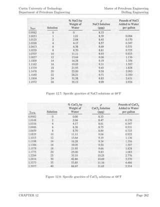
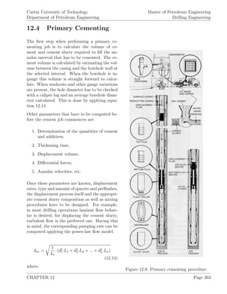
![Curtin University of Technology
Department of Petroleum Engineering
Master of Petroleum Engineering
Drilling Engineering
Lt [ft] ... total depth
dn [in] ... diameter of the nth section
Ln [ft] ... length of the nth section
In conventional primary cementing the cement is displaced through the casing. In order to avoid
contamination of the cement with mud, a so called “spacer” is placed between them. The spacer
in front of the cement, which is also called “preflush”, is commonly water. Water is often chosen
since it is easy to obtain, it can be put in turbulent flow condition at relatively low circulation
rates and it does not affect the setting time of the cement. The column of water pumped ahead
of the cement causes a desired reduction of hydrostatic pressure in the annulus. The volume of
the spacer is given by:
Vspacer = Aan.
∆ph
0.292. (ρm − ρw)
(12.15)
where:
Vspacer [bbl] ... volume of spacer (water)
Aan [ft3
/ft] ... annular capacity
∆ph [psi] ... reduction of hydrostatic pressure
Figure 12.10: Cement Heads, (A) Double plug, (B) Single plug
To calculate the pump rate
to displace the spacer in tur-
bulent flow, the Newtonian
flow model is used.
The procedure of primary
cementing is described as fol-
lows:
To perform the primary ce-
menting job, a device called
“cement head” or “plug con-
tainer”, see figure 12.10, is
mounted on the top joint of
the casing which is hanging
in the elevator. This ce-
ment head serves as connec-
tion from the cement pumps
to the casing. Inside the ce-
ment head, a bottom wiper
plug and a top wiper plug,
see figure 12.11, are placed.
When the cement job is car-
ried out, the bottom plug is released first. It wipes mud off the inside of the casing and keeps
CHAPTER 12 Page 264](https://image.slidesharecdn.com/drillingengineering-160119095813/85/Drilling-engineering-272-320.jpg)
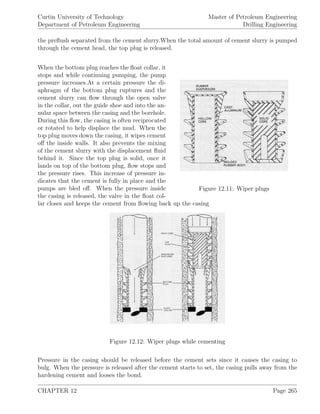
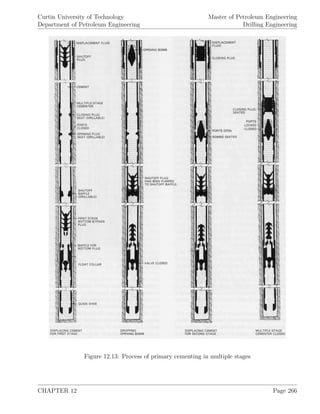
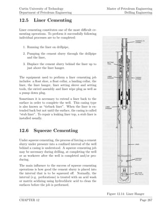
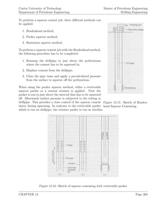
![Curtin University of Technology
Department of Petroleum Engineering
Master of Petroleum Engineering
Drilling Engineering
At the hesitation squeeze method, the cement is squeezed into the desired section with relatively
low pressure while pumping intermittently. The cement is slowly dehydrating and increasing
in viscosity during the non-pumping cycle. This method is used most often to squeeze off low
permeable zones.
12.7 Plugback Cementing
Two different methods for plug cementing operations are encountered in practice: (a) the plugback
cementing and (b) spotting a cement plug at any desired depth of the well. The most common
type, plugback cementing, is used to plug back and abandon deeper zones. Spotting plug ce-
menting is usually performed in open hole sections. To design the spacer and cement slurry, the
same considerations and equations as for primary cementing operations are applied. For the pug
cementing operations a balanced plug techniques that requires pumping a preflush and a spacer
behind the cement, is most often carried out. When the hight of the spacer inside the tubing is
equal to the hight of the preflush, the cement plug is placed balanced.
Cement requirement, water volume to be pumped behind the slurry to balance the plug, plug
length before the pipe is retrieved from the slurry as well as mud volume for pipe displacement
are computed with:
Sacks =
Lplug.Vh
Yield
(12.16)
Vsb =
Vdp.Vsa
Van
(12.17)
where:
Vdp [ft3
] ... volume of drillpipe
Van [ft3
] ... volume of annulus
Lw =
Sacks.Yield
Van + Vdp
(12.18)
where:
Vdp [ft3
/ft] ... capacity of drillpipe
Van [ft3
/ft] ... capacity of annulus
CHAPTER 12 Page 269](https://image.slidesharecdn.com/drillingengineering-160119095813/85/Drilling-engineering-277-320.jpg)
![Curtin University of Technology
Department of Petroleum Engineering
Master of Petroleum Engineering
Drilling Engineering
Vmd = (Ldp − Lw) .Vdp − Vsb (12.19)
where:
Vdp [bbl/ft] ... capacity of drillpipe
Lplug [ft] ... length of desired plug
Vh [ft3
/ft] ... capacity of hole
Vsa [bbl] ... spacer volume ahead of slurry
Vsb [bbl] ... spacer volume behind of slurry
Vmd [bbl] ... volume of mud to displace pipe
CHAPTER 12 Page 270](https://image.slidesharecdn.com/drillingengineering-160119095813/85/Drilling-engineering-278-320.jpg)
![Curtin University of Technology
Department of Petroleum Engineering
Master of Petroleum Engineering
Drilling Engineering
12.8 Examples
1. Cement Class A containing 4 % bentonite is to be mixed. The normal water content of Class
A cement is 46 %, for each added percent of bentonite, 5.3 % of water has to be added. The
specific gravities of cement and bentonite are found to be 3.13 and 2.65 respectively. The weight
of bentonite, the total percent of water to be added as well as the volume of water to be mixed
with one sack of cement, the slurry yield and the slurry density have to be computed.
2. A 7 [in], 29 [lb/ft], N-80 casing has to be cemented in a 9.75 [in] hole for the length of 9,000 [ft].
A 60 [ft] shoe track is to be used and cementing carried out with a Class G, 15.4 [ppg] cement. The
plastic viscosity and the yield point of the cement are 50 [cp] and 10 [lb/ 100 ft] respectively. The
cement is pumped with a duplex pump, having a 18 [in] stroke, a 6.5 [in] liner and a 2.5 [in] rod,
and is operating at 60 [rpm] with an efficiency of 90 %. The water requirement of Class G cement
is 5 [gal/sack] with the slurry volume of 1.15 [ft3/sack]. Since the cement is to be prevented from
contamination with the previously used 11.6 [ppg] drilling mud, 30 [bbl] of fresh water are pumped
as preflush spacer. For cement mixing, a truck with a mixing capacity of 30 [sacks/min] is used.
Calculate the:
(a) Quantity of cement required,
(b) Volume of mixing water,
(c) Total time for the job, allowing 15 minutes for
the release of plug,
(d) Pressure differential prior to pumping the plug,
(e) Flow velocity in the casing and the type of flow,
(f) Flow velocity in the annulus and the type of flow.
3. A 5 [in] OD, 18 [lb/ft] liner (including hanger and float) is to be cemented in a 6-1
4
[in] hole for
a length of 2,000 [ft]. The liner is run in on a 2-7
8
[in], 10.4 [lb/ft] drillpipe to the liner landing
collar at 11,540 [ft]. The total well depth is 11,600 [ft], the liner-wipe plug at 9,615 [ft] and the
top of the liner at 9,600 [ft]. Calculate the:
(a) Sacks of Class E cement required if the
yield is 1.15 [ft3/sack],
(b) Displacement to the liner plug,
(c) Displacement from the liner plug to the landing collar.
4. Within a 6-1
2
[in] hole a 300 [ft] plug is to be placed at 9,000 [ft] using a 2-3
8
[in], 4.6 [lb/ft]
tubing. When 15 [bbl] of water are to be pumped ahead of the slurry that has a yield of 1.5
[ft3/sack], compute the:
CHAPTER 12 Page 271](https://image.slidesharecdn.com/drillingengineering-160119095813/85/Drilling-engineering-279-320.jpg)

![Curtin University of Technology
Department of Petroleum Engineering
Master of Petroleum Engineering
Drilling Engineering
Bibliography
[1] Aadnoy B.S., “Modern Well Design”, A.A Balkema, Rotterdam, (1996), 240 pages.
[2] Baker R., “A Primer of Oil-Well Drilling, Fourth Edition”, Petroleum Extension Ser-
vice, University of Texas, Austin TX, (1979), 94 pages.
[3] Baker R., “A Primer of Offshore Operations, Second Edition”, Petroleum Extension
Service, University of Texas, Austin TX, (1985), 114 pages.
[4] Bourgoyne A.T. Jr., Millheim K.K., Chenevert M.E., Young F.S., “Applied Drilling En-
gineering”, SPE Textbook Series, Vol 2, (1991), 502 pages.
[5] Craft B.C., Holden W.R., Graves E.D., “Well Design: Drilling and Production”,
Prentice-Hall Inc., Englewood Cliffs New Jersey, (1962), 571 pages.
[6] Darley H.C.H., Gray G.R., “Composition and Properties of Drilling and Completion
Fluids, Fifth Edition”, Gulf Publishing Company, Houston TX, (1988), 643 pages.
[7] Devereux S., “Drilling Technology in nontechnical language”, PennWell Publishing,
Tulsa Oklahoma, (1999), 337 pages.
[8] Earlougher R.C. Jr., “Advances in Well Test Analysis”, Monograph Volume 5 of the
Henry L. Doherty Series, (1977), 264 pages.
[9] Economides M.J., Watters L.T., Dunn-Norman S., “Petroleum Well Construction”, John
Wiley & Sons Publishing, (1998), 622 pages.
[10] ETA Offshore Seminars, Inc. “The Technology of Offshore Drilling, Completion and
Production”, The Petroleum Publishing Company, Tulsa Oklahoma, (1976), 426 pages.
[11] Gabolde G., Nguyen J.-P., “Drilling Data Handbook, Sixth Edition”, Institut Francais
du Petrole, Gulf Publishing Company, Houston TX, (1991), 533 pages.
[12] Hallibuton, “Technology Exchange Session, 1992”, (1992).
[13] Harris L.M., “An Introduction to Deepwater Floating Drilling Operations”, PPE
Books, Petroleum Publisjinh Company, Tulsa Oklahoma, (1972), 272 pages.
[14] Hughes Tool Company, “Drilling Manual”, Section B, care, handling & specifications for
tool joints, drill pipe, casing & tubing, (1969),
CHAPTER 12 Page 273](https://image.slidesharecdn.com/drillingengineering-160119095813/85/Drilling-engineering-281-320.jpg)
![Curtin University of Technology
Department of Petroleum Engineering
Master of Petroleum Engineering
Drilling Engineering
[15] Lapeyrouse N.J., “Formulas and Calculations for Drilling, Production and
Workover”, Gulf Publishing Company, Houston TX, (1992), 216 pages.
[16] Maurer W.C., “Advanced Drilling Techniques”, Petroleum Publishing Company, Tulsa
Oklahoma, (1980), 698 pages.
[17] Mian M.A., “Petroleum Engineering Handbook For The Practicing Engineer, Vol
II”, PennWell Publishing, Tulas Oklahoma, (1992), pp. 271-453.
[18] Mitchell B., “Advanced Oilwell Drilling Engineering Handbook”, Oilwell Drilling,
Golden Colorado, (1974), 605 pages.
[19] Moore P.L., “Drilling Practices Manual, Second Edition”, PennWell Publishing, Tulsa
Oklahoma, (1986), 586 pages.
[20] Mouchet J.P., Mitchell A., “Abnormal pressures while drilling, Origins - Predictions
- Detection - Evaluation”, elf aquitaine, manuels techniques 2, (1989), 255 pages.
[21] Short J.A., “Drilling and Casing Operations”, PennWell Publishing, Tulsa Oklahoma,
(1982), 426 pages.
[22] Short J.A., “Prevention, Fishing & Casing Repair”, PennWell Publishing, Tulsa Okla-
homa, (1995), 559 pages.
[23] SPE Reprint Series, “Well Completions”, No. 5, (1970), 41 articles, 344 pages.
[24] SPE Reprint Series, “Drilling”, No. 22, (1987), 33 articles, 348 pages.
[25] SPE Reprint Series, “Directional Drilling”, No. 30, (1990), 23 articles, 208 pages.
[26] SPE Reprint Series, “Coiled-Tubing Technology”, No. 38, (1994), 20 articles, 176 pages.
[27] Whittaker A., “Mud Logging Handbook”, Prentice Hall, Englewood Cliffs New Jersey,
(1991), 531 pages.
CHAPTER 12 Page 274](https://image.slidesharecdn.com/drillingengineering-160119095813/85/Drilling-engineering-282-320.jpg)

This document provides an overview of drilling engineering topics taught in the Master of Petroleum Engineering program at Curtin University of Technology. It covers the components and operation of rotary drilling rigs, geomechanics considerations for wellbore stability, drilling hydraulics, drill bits, drillstring design, and drilling fluids. The document is divided into chapters that describe key aspects of each topic in detail.


