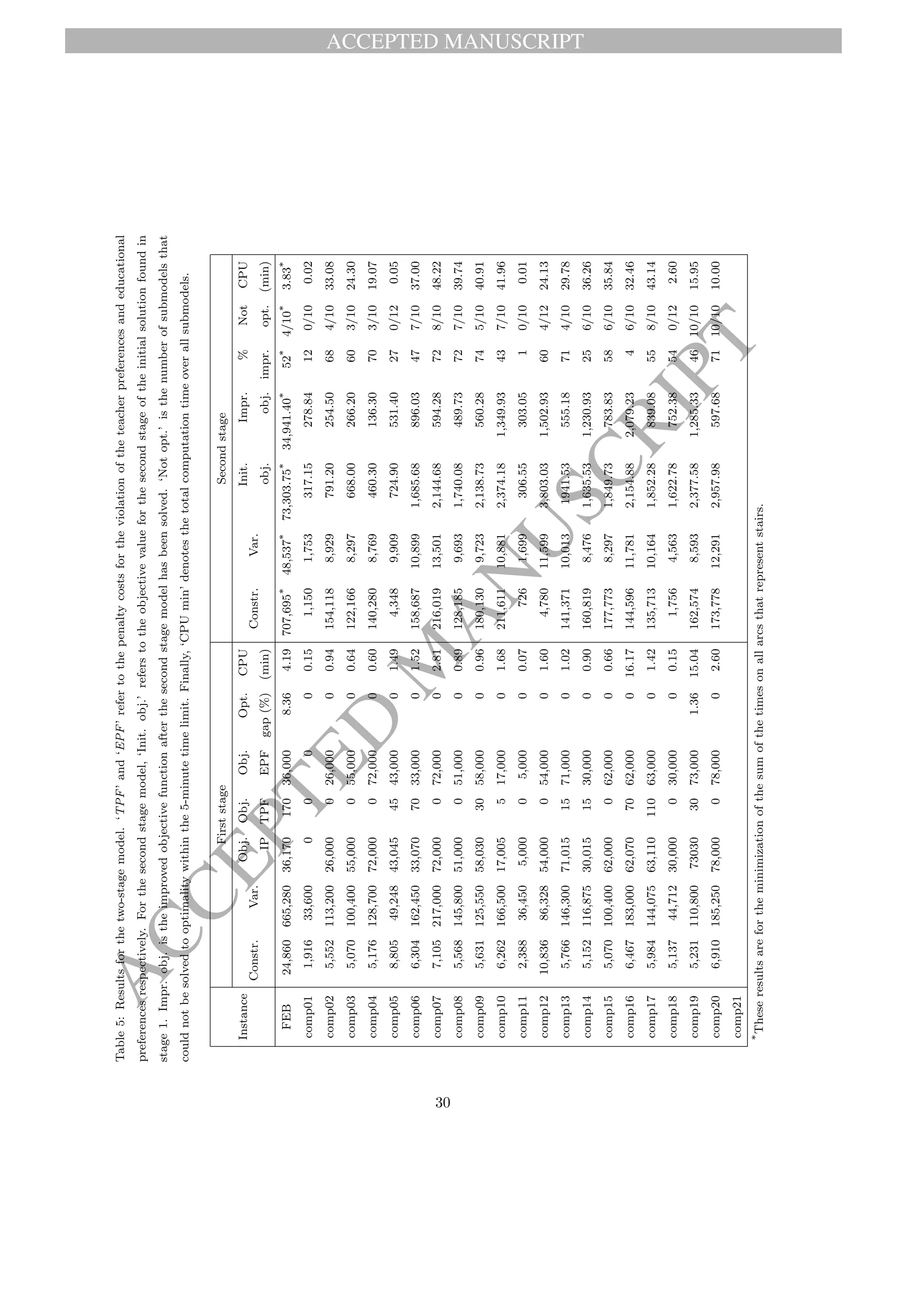
Accepted Manuscript
Developing compact course timetables with optimized student flows
Hendrik Vermuyten, Stef Lemmens, Inˆes Marques, Jeroen Beli¨en
PII: S0377-2217(15)01077-2
DOI: 10.1016/j.ejor.2015.11.028
Reference: EOR 13379
To appear in: European Journal of Operational Research
Received date: 30 April 2015
Revised date: 20 November 2015
Accepted date: 23 November 2015
Please cite this article as: Hendrik Vermuyten, Stef Lemmens, Inˆes Marques, Jeroen Beli¨en, Develop-
ing compact course timetables with optimized student flows, European Journal of Operational Research
(2015), doi: 10.1016/j.ejor.2015.11.028
This is a PDF file of an unedited manuscript that has been accepted for publication. As a service
to our customers we are providing this early version of the manuscript. The manuscript will undergo
copyediting, typesetting, and review of the resulting proof before it is published in its final form. Please
note that during the production process errors may be discovered which could affect the content, and
all legal disclaimers that apply to the journal pertain.
ACCEPTED MANUSCRIPT
ACCEPTED
M
ANUSCRIPT
Highlights
• A course timetable has an impact on the student flows between consecutive
lectures.
• Large flows lead to congestion and large travel times between lectures.
• Therefore, we look at minimizing the travel time between consecutive
lectures.
• Flows are modeled in a detailed way, using insights from pedestrian traffic
models.
• Using a decomposition approach, our model can be solved with a standard
IP solver.
1
ACCEPTED MANUSCRIPT
ACCEPTED
M
ANUSCRIPT
Developing compact course timetables with optimized
student flows
Hendrik Vermuytena,∗
, Stef Lemmensb
, Inˆes Marquesc,d,e
, Jeroen Beli¨ena
aResearch Center for Quantitative Business Processes, Faculty of Economics and Business,
KU Leuven Campus Brussels, Warmoesberg 26, 1000 Brussels, Belgium
bResearch Center for Operations Management, Department of Decision Sciences and
Information Management, Faculty of Business and Economics, KU Leuven, Naamsestraat
69, 3000 Leuven, Belgium
cDepartamento de Estat´ıstica e Investiga¸c˜ao Operacional, Faculdade de Ciˆencias,
Universidade de Lisboa, 1749-016 Lisboa, Portugal
dECEO, Universidade Lus´ofona de Humanidades e Tecnologias, 1749-024 Lisboa, Portugal
eCentro de Matem´atica, Aplica¸c˜oes Fundamentais e Investiga¸c˜ao Operacional, Faculdade de
Ciˆencias, Universidade de Lisboa, 1749-016 Lisboa, Portugal
Abstract
In university buildings with many rooms spread over different floors, large stu-
dent flows between two consecutive lectures might cause congestion problems.
These congestions result in long queues at elevators or at stairwells, which might
lead to delays in lecture starts. The course timetable clearly has an important
impact on these congestions. This paper presents a two-stage integer program-
ming approach for building a university course timetable that aims at mini-
mizing the resulting student flows. The first stage minimizes the violation of
the teacher and educational preferences by assigning lectures to timeslots and
rooms. The second stage reassigns classrooms to lectures of the timetable of the
first stage and minimizes the student flow. The conceptual model is applied to
the dataset of the Faculty of Economics and Business of the KU Leuven Cam-
pus Brussels and is tested and validated with 21 adapted instances from the
literature. In contrast to a monolithic model, the two-stage model consistently
succeeds in finding good quality feasible solutions. Moreover, the generated
∗Corresponding author
Email addresses: hendrik.vermuyten@kuleuven.be (Hendrik Vermuyten),
stef.lemmens@kuleuven.be (Stef Lemmens), ines.marques@fc.ul.pt (Inˆes Marques),
jeroen.belien@kuleuven.be (Jeroen Beli¨en)
Preprint submitted to European Journal of Operational Research December 3, 2015
ACCEPTED MANUSCRIPT
ACCEPTED
M
ANUSCRIPT
timetables entail significantly reduced student flows compared to the flows of
the manually developed course timetable.
Keywords: Scheduling, Timetabling, University course timetabling problem,
Student flow, Integer programming
1. Introduction
The growing student numbers at colleges and universities have resulted in
an enlarged complexity in terms of planning and organization. One of the tasks
that becomes increasingly complex is the development of course timetables.
Daskalaki et al. [1] define the University Course Timetabling Problems (UCTP)5
as the construction of a weekly timetable in which all operational rules and
requirements of the academic institution are met and as many wishes as possible
of the staff and students are satisfied. According to Carter and Laporte [2] the
UCTP can be formulated as a multi-dimensional assignment problem. Students
and lecturers need to be assigned to lectures which are in turn assigned to rooms10
and timeslots such that no overlap occurs. Course timetables have to satisfy
various requirements of different stakeholders including non-overlap of courses,
free hours, lecturers’ preferences, student preferences, etc. Furthermore, the
course timetable can have a huge impact on queues in stair halls and elevators,
particularly for universities or colleges with many students that follow courses15
in a single building. The congestion problems in stair halls and elevators are
caused by traveling students that all have to switch rooms at the same time
between two consecutive lectures. Clearly, student flows can be controlled and
monitored via the course timetables. For example, if the schedules are arranged
so that consecutive lessons take place in rooms situated on the same floor (or on20
a floor as close as possible), there will be far fewer queues at the elevators and in
the stairwells. Thus, next to the various constraints and preferences of different
stakeholders, the resulting student flows should also be taken into account when
building the course timetable.
This research was motivated by the UCTP at the KU Leuven Faculty of25
3
ACCEPTED MANUSCRIPT
ACCEPTED
M
ANUSCRIPT
Economics and Business (FEB) campus Brussels. As described in Mercy [3] the
FEB campus Brussels has gone through a process of campus consolidation in
which several buildings at different locations in Brussels have been sold and the
lectures of all economic programs have been concentrated at a single location
in the center of Brussels. As a result, over 8000 students daily follow classes in30
a single building, which inevitably causes major congestion problems at the el-
evators and the stairwells during lecture transitions. This congestion is already
alleviated by assigning different starting times for the academic and professional
programmes. However, long waiting times and difficult passages remained to
exist. Student flows could also be minimized by maximally spreading the lec-35
tures over the day and over the week. However, students and teachers are often
dissatisfied with a timetable with free periods in-between. Being not able to at-
tend or to teach lectures consecutively requires more time for traveling towards
and away from classrooms. Commuting students especially often prefer to have
a compact timetable instead of having free time between lectures. Particularly,40
days with only one scheduled lecture should be avoided.
Despite the large complexity in building UCTPs, many educational institutes
still develop their UCTP manually, which requires a lot of time and creativity of
the planners. It is nearly impossible for human planners to solve the enormous
puzzle taking into account the constraints and preferences of all stakeholders, let45
alone to incorporate the resulting student flows. After showing that a monolithic
integer programming (IP) model is intractable for a state-of-the-art commercial
solver for solving real-life UCTPs taking into account student flows, this paper
presents a two-stage IP approach. In the first stage, lectures are assigned to
timeslots taking into account the various constraints and maximizing the stake-50
holders’ preferences. The second stage uses the timetable of the previous stage
as input and reassigns the classrooms with the objective of minimizing the re-
sulting student flows. Through extensive computational tests, we show that,
in contrast to a monolithic IP, this two-stage IP approach is capable of finding
good quality solutions with minimized student flows for real-life UCTPs.55
The remainder of this paper is organized as follows: Section 2 discusses
4
ACCEPTED MANUSCRIPT
ACCEPTED
M
ANUSCRIPT
related literature of different timetabling problems, modeling and solving tech-
niques. Section 3 introduces the timetabling problem of the KU Leuven Campus
Brussels. Next, a mathematical formulation for the problem is discussed in Sec-
tion 4, followed by a discussion of the solution method used in Section 5. Section60
6 subsequently applies the model to the data of the Faculty of E&B of the KU
Leuven Campus Brussels. The latter section also reports on results from tests
using data available from the literature. Section 7 concludes this paper and lists
directions for future research.
2. Literature Review65
In the following subsections, we first give an overview of the solution tech-
niques that have been developed in the literature. Next, we look at the issue of
compact timetables, where free hours between consecutive lectures are avoided
as much as possible as this is preferred by most students and staff. In the third
subsection, we discuss the literature on the incorporation of student flows into70
the timetabling problem. In the last subsection, we outline the approach taken
in this paper.
2.1. Solution Techniques
Various methods have been proposed for automating the development of
course timetables ([4]). Overviews were given by Carter and Laporte ([5], [2]),75
Schaerf [6], Burke and Petrovic [7], Petrovic and Burke [8], Lewis [9], MirHassani
and Habibi [10] and Babaei et al. [11]. Below, we discuss three approaches that
are most widely used for course timetabling in more detail, namely graph color-
ing, metaheuristic approaches, and mathematical programming. Other solution
approaches include constraint logic programming (e.g., Gu´eret et al. [12]), case-80
based reasoning (e.g., Burke et al., [13] and [14]), and neural networks (e.g.,
Carrasco and Pato [15]).
Graph coloring approaches are often used for timetabling thanks to the ease
of implementation (Petrovic and Burke [8]). In graph coloring approaches the
5
ACCEPTED MANUSCRIPT
ACCEPTED
M
ANUSCRIPT
timetabling problem is modeled as a graph in which the nodes correspond to85
the events (lectures) and the arcs correspond to the event-clash constraints (De
Causmaecker et al., [16]). Next, each node needs to be assigned to a color,
which represents a timeslot, such that connected nodes have a different color.
The goal is to find a solution in which the number of colors used does not exceed
the number of available timeslots (Lewis [9]).90
Metaheuristics start with one or a set of solutions which are iteratively im-
proved using local search operators with a protection mechanism that avoids
getting stuck in a local optimum. Recent examples of metaheuristic approaches
applied to UCTPs can be found in De Causmaecker et al. [16], L¨u and Hao
[17], Aladag et al. [18], Zhang et al. [19] and Geiger [20]. A hyperheuristic is a95
framework in which an upper-level metaheuristic selects the most appropriate
heuristic out of a set of lower-level heuristics to solve a particular optimization
problem (Petrovic and Burke, [8]). Hyperheuristics are a growing research topic
for tackling timetabling problems (Burke and Petrovic [7]). Hybrid approaches
combine different techniques, for instance Bellio et al. [21] present a hybrid local100
search approach, while Gunawan and Kien Ming [22] propose a hybrid approach
that combines Lagrangian relaxation and simulated annealing.
In the past, due to computational difficulties the use of mathematical pro-
gramming for solving UCTPs has been limited to small size instances. However,
thanks to strong advances in computer software and hardware, and in IP formu-105
lations, mathematical programming approaches for timetabling problems have
become more popular ([1], [23]). Examples of IP formulations for UCTPs can be
found in [24], [1], [25] and [26]. One advantage of mathematical programming
approaches is the ease of incorporating additional soft constraints ([2]).
Unfortunately, UCTPs continue to cause problems for the planning depart-110
ments of universities and colleges, because implementations of the proposed
solution techniques are scarce. According to McCollum [27] this is due to in-
complete data and the difficulty of incorporating implicit knowledge about the
preferences of lecturers and the scheduling policies. There are a few notable
exceptions. Daskalaki et al. [1] apply an integer programming model to the115
6
ACCEPTED MANUSCRIPT
ACCEPTED
M
ANUSCRIPT
timetabling problem of the department of Electrical and Computer Engineering
at the University of Patras. De Causmaecker et al. [16] use a decomposed meta-
heuristic approach to solve the timetabling problem for the KaHo Sint-Lieven
School of Engineering. Dimopoulo and Miliotis [24] report on the implementa-
tion of a computer system for the joint development of a course and examination120
timetable at The Athens University of Economics and Business. Schimmelpfeng
and Helber [26] describe the implementation of an integer programming ap-
proach to create a complete timetable of all courses for a term at the School of
Economics and Management at Hannover University. Badri [28] develops a two-
stage optimization model to solve a faculty-course-time timetabling problem at125
United Arab Emirates University. Finally, Al-Yakoob et al. ([29] and [30]) use
integer programming to obtain, respectively, a course and exam timetable at
Kuwait University.
As shown in this paper, computational difficulties inherent to huge IP models
can be overcome by decomposing the problem in separate stages that can be130
solved efficiently with state-of-the-art IP solvers. Badri [28] also uses a two-
stage multi-objective scheduling model for the assignment of faculty members
to courses and timeslots. Four types of preferences, each with an associated
priority, are grouped into one objective function: the load requirement for each
faculty, the satisfaction of the number of available classrooms, the number of135
evening classes and personal preferences of faculties with respect to course-time
assignments. The results of the first stage, the faculty-course assignments, are
the input for the second stage. The second stage assigns faculties to timeslots.
Burke et al. [31] propose a general framework for the decomposition of large
problems into multiple restricted submodels, which only consider a subset of140
the objectives at first. The solutions to the subproblems are then aggregated to
obtain feasible solutions to the original problem. An advantage to their method
is that it is easily implemented using a general IP solver and provides bounds
on the solution quality.
7
ACCEPTED MANUSCRIPT
ACCEPTED
M
ANUSCRIPT
2.2. Compact Timetables145
Students and teachers often prefer compact timetables. A compact timetable
refers to the absence of free hours between consecutive lectures. Below we de-
scribe three contributions that also focus on compact timetables. Santos et al.
[32] include constraints regarding the number of free periods in the timetables
of the teachers. A compact and an extended formulation are proposed. The au-150
thors use cut and column generation to increase the dual bounds of the extended
formulation. Dorneles et al. [33] present a mixed integer linear programming
model to a high school timetabling problem. Among the different requirements
that are considered in Brazilian schools, two compactness constraints must be
met on a teacher’s schedule: the minimization of working days and the avoid-155
ance of idle timeslots. The authors propose a fix-and-optimize heuristic com-
bined with a variable neighbourhood descent method using three different types
of decomposition (class, teacher and day). Burke et al. [31] distinguish four
penalty terms: classroom capacity, spread of the lectures of a course, time com-
pactness and classroom stability. The penalization of classroom capacity and160
stability is respectively done by penalizing classrooms if insufficient seats are
available and distinct classrooms are used for different lectures of a course. The
spread of the lectures is penalized when the actual spread is smaller than the
prescribed spread. For a given curriculum, every time a lecture is not adjacent
(an isolated lecture) to another lecture on the same day, time compactness is165
penalized.
2.3. Student Flows
As mentioned earlier, the motivation of this paper is the congestion that
occurs in the corridors and at the stairwells at the Faculty of Economics and
Business at KU Leuven Campus Brussels and the observation that the timetable170
has an impact on this. Therefore, we discuss previous work that incorporates
the traveling of students between consecutive lectures into the timetabling prob-
lem. To the best of our knowledge, the studies in [29], [30], [34], [35], [36], and
8
ACCEPTED MANUSCRIPT
ACCEPTED
M
ANUSCRIPT
[37] are the only ones that, to a limited extent, incorporate student flows. Al-
Yakoob and Sherali [29] present a Mixed Integer Programming (MIP) model175
for class timetabling problems and consider a related congestion topic. The
authors address the problem of parking and traffic congestions for students and
faculty members when lectures are inadequately spread over all the available
timeslots. Students and faculty members are adequately spread over all the
available timeslots by constraints that impose an upper bound on the number180
of students that follow classes (take exams) during each timeslot. These bounds
are not necessary the same for different timeslots. For example, the timeslots
when employees and staff start and finish working can have a smaller upper
bound. Student flows are also taken into account by Al-Yakoob et al. [30].
The authors present a MIP for exam timetabling and address the same topics:185
parking and traffic congestions and an inadequately spread of the exams. There-
fore, scheduling consecutive exams at distant campuses is undesirable. Parking
and traffic congestions are addressed by imposing a constraint on the number
of students that can be involved in one exam period. Pongcharoen et al. [34]
present a stochastic optimization model for the UCTP. They tackle the problem190
of student movement by a soft constraint ensuring that students attend lectures
in the same classroom as much as possible. More recently, Ferdoushi et al.
[35] also consider the minimization of the movement of students between rooms
through soft constraints. The authors develop a modified hybrid particle swarm
optimization approach to a highly constrained realistic environment in the Com-195
puter Science and Engineering department of Khulna University of Engineering
& Technology, Bangladesh. In both papers, distances between classrooms are
not taken into account. Hertz [36] uses tabu search and graph theory for solving
timetabling problems. In addition to the classical feasibility constraints of the
timetable, precedence requirements and geographical constraints are taken into200
account. Precedence requirements are, for example, lectures which should be fol-
lowed by exercise sessions in the same day. Geographical constraints are related
to the distance of two classrooms of two consecutive lectures. The objective
function penalizes infeasible timetables and pairs of consecutive lectures at dis-
9
ACCEPTED MANUSCRIPT
ACCEPTED
M
ANUSCRIPT
tant classrooms. Rudov´a et al. [37] use a generic iterative forward search and205
a branch-and-bound algorithm for a complex university timetabling problem.
They develop a generic method that is not specifically tailored to a single prob-
lem type so that it can be used in practice to solve different real-life timetabling
problems with different constraints. The authors also consider the distances be-
tween rooms and penalize class assignments that require students or instructors210
to travel large distances between consecutive lectures.
2.4. Outline Of The Current Article
The approach presented in this paper aims to develop compact timetables for
which the resulting students flows are minimized in order to avoid congestions
in the corridors and at the stairways. To achieve the former objective, two-hour215
free time periods are prevented by a hard constraint. To achieve the latter
objective, the flow of students between consecutive lectures is modeled in detail
using a graph that represents the faculty building, where the flow through each
arc and the resulting travel times are optimized by changing the assignment of
lectures to rooms.220
Our method will be tested on a real-life case as well as on instances avail-
able in the literature. International timetabling competitions (ITC) regularly
provide a number of benchmark problems that are widely used in timetabling
literature to develop computational experiments. Badoni et al. [38] describe a
hybrid algorithm combining a genetic algorithm with local search using events225
based on groupings of students to solve a UCTP. The authors applied their algo-
rithm on instances based on the datasets from the first international timetabling
competition (ITC2002). Hao and Benlic [39] combine tabu search and IP for
finding new lower bounds for the ITC2007 curriculum based course timetabling
problem. Phillips et al. [25] validate their IP model for solving a UCTP through230
a real-life case at the University of Auckland and on instances from the ITC2007.
Dorneles et al. [33] used the ITC2011 instances to test their algorithm dedicated
to a high school timetabling problem.
10
ACCEPTED MANUSCRIPT
ACCEPTED
M
ANUSCRIPT
3. Problem Description
3.1. The KU Leuven Campus Brussels Timetabling Problem235
In the timetabling problem for the KU Leuven Campus Brussels, a weekly
timetable needs to be built, where lectures (events) need to be assigned to
timeslots and rooms. Two things need to be taken into account:
• Teachers are already assigned to lectures.
• A series is a group of students that have exactly the same timetable. For240
each series, it is known in advance how many students there are in the
series and which lectures they need to attend.
Series are divided in four different types of education: daytime education,
morning education, evening education and evening education only on Tuesday
and Thursday. The number of available timeslots for a series depends on the245
type of education of the series. These Educational Preferences (EPF) can be
violated by scheduling a lecture at a timeslot when some student series are
unavailable to attend this lecture due to their type of education.
Every teacher can submit his teaching preferences regarding the timeslots
at the start of the academic year. These Teacher Preferences (TPF) can be250
violated by scheduling a lecture at a timeslot when a teacher does not prefer to
teach this lecture. A first objective is then the minimization of the violation of
the aforementioned teacher preferences and educational preferences.
An additional concern in building the timetable for the KU Leuven Campus
Brussels, is the congestion caused by students traveling from one classroom255
to another in between consecutive lectures. A consequence of this congestion
is that lectures often start late because it takes a lot of time for students to
travel to their next classroom. Therefore, we include the minimization of the
maximum of the travel time for each series of students for all timeslots as a
second objective.260
11
ACCEPTED MANUSCRIPT
ACCEPTED
M
ANUSCRIPT
3.2. Incorporating Student Flows
To model the flow and resulting travel times of students, we employ some of
the modeling techniques used in traffic assignment models. Traffic assignment
models try to predict traffic flows and the resulting congestion and travel times
on each route in the network, given the estimated number of people who want265
to travel between different origin-destination pairs [40]. They represent the road
network as a graph G = (N, A), where the set N of nodes represents destinations
or junctions and the set A of arcs the roads between them. Analogously, to
model the flow and resulting travel times of students, we represent the layout of
the building by a graph in which a number of adjacent classrooms are grouped270
into a single node. The number of classrooms that are combined into one node
is based on a trade-off between the complexity of the model on the one hand
and its realism on the other hand. Next, only nodes which represent physical
locations that are adjacent to each other in the actual building are connected
by an arc, through which a ‘flow’ of students can pass. This implies that it275
is possible that students who travel from some classroom A to some classroom
B have to pass through multiple arcs to reach their destinations (e.g., if they
have to travel from the 3rd floor to the 5th floor, they need to pass through
the arc for the stairs between the 3rd and 4th floor first, and then through the
arc for the stairs between the 4th and 5th floor). Secondly, in reality it can be280
that there are multiple routes one can take to reach the same destination from
a given location. Therefore, in the model a route choice probability has to be
specified to determine the percentage of students that will cause flow in each
possible arc of a certain route. Figure 1 gives an example of layout of a building
and the corresponding graph to model the student flows.285
An important element in the analysis of traffic assignment models is the no-
tion of congestion [40]. As traffic volume on an arc increases, the average travel
speed on the link decreases, until a situation of total congestion is reached. The
travel time of a link is modeled with a link performance function, which relates
the travel time through a link to the volume of traffic on that link. A similar con-290
cept has been observed for pedestrian flows. In the literature this relationship
12
ACCEPTED MANUSCRIPT
ACCEPTED
M
ANUSCRIPT
Figure 1: An example of a building layout and the corresponding graph. In this building,
there are 7 classrooms. Rooms A and B are assigned to node 1, rooms C and D to node 3,
rooms E and F to node 4 and room G to node 6. Rooms E, F, G and the entrance are on the
first floor and rooms A, B, C and D are on the second floor, so arc (2, 5) represents stairs. It
is clear that in this specific layout only one route can be taken between any two classrooms.
between crowd density and walking speed is called the ‘fundamental diagram’,
because of its importance in models describing human walking behavior (for a
general overview of the pedestrian walking behavior research, see e.g. [41] and
[42]). Since we are interested in the travel time of students between classrooms,295
we will describe this concept in more detail.
Schadschneider & Seyfried [43] give an overview of the state of empirical
research and examine the data relating to the fundamental diagram. Their
data only consider planar walking facilities such as corridors and do not apply
to stairs. They observe that there is a lot of variance in the data, which has300
been attributed to a variety of factors. Secondly, there is no consensus whether
there is even any significant difference between uni- and multidirectional flows.
Therefore, we do not distinguish between uni- and bidirectional flows through
an arc.
Based on the data in [43], we assume the following relationship between
13
ACCEPTED MANUSCRIPT
ACCEPTED
M
ANUSCRIPT
crowd density ρ, and walking speed v, i.e.
v(ρ) =
α
ρ
, (1)
where α is a scaling parameter. The reason for this choice is that the travel time
as a function of crowd density is then linear. Another possibility is of course
to assume a linear relationship between crowd density and walking speed, and
afterwards fit a piecewise linear function to the resulting nonlinear travel time
function. There are, however, two arguments to support our choice: (i) at
high crowd densities, walking speed does not actually reach zero, but ‘turbulent
crowd movements’ are observed [44], and (ii) in traffic assignment models it
has been observed that asymptotic travel time functions empirically lead to
unrealistically high travel times [45]. Other empirical studies have looked at the
fundamental diagram for the movement on stairs. As expected, walking speed
here is lower than on planar surfaces, see e.g. [46]. Therefore, we include a
correction term γ ∈ [0, 1], such that
v(ρ) = γ
α
ρ
. (2)
Then the travel time through arc (i, j) is the length of the physical location
represented by this arc divided by the walking speed of the students walking
through it; that is, it depends on the total flow of students going through the
arc:
Tarc
tij (ρ) =
lengthij
v(ρ)
=
lengthij
α
ρ +
lengthij
vmax
. (3)
The second term in equation (3) ensures a minimal travel time when the density
is zero. Furthermore, the crowd density ρ at time t equals the number of students
that travel through arc (i, j) at time t, denoted by Ftij , divided by the surface
area of the physical location represented by this arc, i.e.
ρ =
Ftij
areaij
. (4)
This representation can also be extended to a situation where there are305
multiple buildings. In this case, it suffices to define an arc between the entrances
14
ACCEPTED MANUSCRIPT
ACCEPTED
M
ANUSCRIPT
of each pair of buildings and assume a fixed travel time for that arc, since in
public spaces and roads the density is ‘given’ and only marginally influenced by
the number of traveling students.
4. MIP formulation310
Building on the explanation of the previous section, we are now able to derive
a mixed integer programming formulation for our model to jointly minimize the
violation of teacher and educational preferences on the one hand and the travel
times of students on the other hand.
4.1. Notation315
• Constants
– δ: number of available timeslots in one day. This number is assumed
to be the same for every day that lectures can be scheduled.
• Sets
– c, d ∈ C: classrooms. Every lecture needs a classroom of the correct320
type and with sufficient capacity. Different types of classrooms, for
example PC-rooms and laboratories, can exist.
– i, j ∈ N: nodes
– k ∈ K: days. These are the days (Monday=1, ..., Friday=5) that
lectures can be scheduled.325
– l, m ∈ L: lectures. Every lecture takes two hours, is unique and is
scheduled once. A course that consists of, for example, two lectures
is scheduled twice.
– p ∈ P: paths
– r ∈ R: teachers330
– s ∈ S: series of students
15
ACCEPTED MANUSCRIPT
ACCEPTED
M
ANUSCRIPT
– t ∈ T: available timeslots. These are the different time periods that
a lecture can be scheduled.
• Subsets
– Cl : classrooms that can be used to schedule lecture l335
– LC
c : lectures that can be scheduled in classroom c
– LR
r : lectures that are taught by teacher r
– LS
s : lectures that need to be attended by series s
– Pcd : all paths that connect room c and room d
– Tk : timeslots on day k340
• Parameters
– apcd : percentage of students who use path p to travel from room c to
room d
– bijp: equals 1 if arc (i, j) is on path p, 0 otherwise
– clt : penalty cost for scheduling lecture l in timeslot t. These costs345
include both the teacher preferences and educational preferences.
– ns: number of students in series s
• Decision variables
– xltc ∈ {0,1}: equals 1 if lecture l is scheduled at time t in room c, 0
otherwise350
– Utsp ∈ [0,1]: the percentage of students from series s who use path p
at time t
– Ftij ≥ 0: the total student flow through arc (i, j) at time t
– Tarc
tij ≥ 0: the travel time through arc (i, j) at time t
– Ttotal
tsp ≥ 0: the total travel time for those students of series s that355
use path p at time t
– Tmax = maxt,s,p{Ttsp}
16
ACCEPTED MANUSCRIPT
ACCEPTED
M
ANUSCRIPT
4.2. The Model
The first set of constraints ensure a feasible timetable. These are hard con-
straints. Constraint set (5) implies that every lecture has to be scheduled in a
feasible timeslot and classroom. Constraints (6) guarantee that every teacher
can teach at most one lecture at a particular timeslot. This lecture is able to
be taught by this teacher and is scheduled in a feasible timeslot. Constraint set
(7) ensures that, for each timeslot, at most one feasible lecture can be scheduled
in each classroom. A series of students can only attend one lecture at a time.
This is implied by constraint set (8).
∀l ∈ L :
t∈T c∈Cl
xltc = 1 (5)
∀r ∈ R, ∀t ∈ T :
l∈LR
r
c∈Cl
xltc ≤ 1 (6)
∀t ∈ T, ∀c ∈ C :
l∈LC
c
xltc ≤ 1 (7)
∀s ∈ S, ∀t ∈ T :
l∈LS
s
c∈Cl
xltc ≤ 1 (8)
Labour legislation also enforces a number of constraints regarding the work-
ing hours of teachers. The first constraint is that teachers cannot teach more
than ∆1 lectures of two hours per day. Constraints (9) ensure these terms of
employment. Next, teachers are also not allowed to teach more than ∆2 lectures
consecutively. This is enforced by constraints (10). Here Q denotes a subset of
consecutive timeslots.
∀r ∈ R, ∀k ∈ K :
l∈LR
r
t∈Tk c∈Cl
xltc ≤ ∆1 (9)
∀r ∈ R, ∀k ∈ K, ∀Q ⊂ Tk , |Q| = ∆2 + 1 :
l∈LR
r
t∈Q c∈Cl
xltc ≤ ∆2 (10)
Furthermore, teachers are not allowed to teach in the first timeslot if they taught
in the last timeslot on the previous day. Constraint set (11) shows how this
prohibition is enforced. Finally, the legislator does not allow that a docent
teaches in the first and last timeslot of a particular day. This is implied by
17
ACCEPTED MANUSCRIPT
ACCEPTED
M
ANUSCRIPT
constraint set (12).
∀r ∈ R, ∀k ∈ {1, ..., |K| − 1} :
l∈LR
r
c∈Cl
(xl,kδ,c + xl,kδ+1,c) ≤ 1 (11)
∀r ∈ R, ∀k ∈ K :
l∈LR
r
c∈Cl
(xl,1+(k−1)δ,c + xl,kδ,c) ≤ 1 (12)
Constraints (13) are the compactness constraints: these constraints avoid two-
hour free periods in the timetables. If a lecture is scheduled at timeslots t and
t + 2 of a particular day, then another lecture needs to be scheduled at timeslot
t + 1 of the same day.
∀s ∈ S, ∀k ∈ K, ∀t ∈ {δ(k − 1) + 1, ..., δk − 2} :
l∈LS
s
c∈Cl
(xltc + xl,t+2,c − xl,t+1,c) ≤ 1 (13)
The second set of constraints determines the student flows. For every series
of students s we need to determine which paths they use given the assignment
of lectures to classrooms. To this end, Utsp indicates the percentage of students
from series s that use path p at time t. The relationship between xltc and Utsp
is then as follows:
∀t ∈ {1, ..., |T| − 1}, ∀s ∈ S, ∀l, m ∈ LS
s , ∀p ∈ P, ∀c ∈ Cl , d ∈ Cm :
Utsp ≥ apcd (xltc + xm,t+1,d − 1) (14)
However, we also need to include the flow caused by students who leave the
building when they do not have class at time t + 1, and students who enter the
building when they did not have class at time t. The following two expressions
include the first and second type of flow respectively:
∀t ∈ {1, ..., |T| − 1}, ∀s ∈ S, ∀l ∈ LS
s , ∀p ∈ P, ∀c ∈ Cl :
Utsp ≥ apc,exit

xltc −
m∈LS
s
d∈Cm
xm,t+1,d

 (15)
Utsp ≥ apc,exit

xl,t+1,c −
m∈LS
s
d∈Cm
xmtd

 (16)
18
ACCEPTED MANUSCRIPT
ACCEPTED
M
ANUSCRIPT
Then, the flow through each arc (i, j) at time t can be calculated as follows:
∀t ∈ T, ∀i, j ∈ N : Ftij =
p∈P s∈S
nsbijpUtsp (17)
To assure that crowd density does not reach hazardous levels (see e.g. [44]),
the flow through an arc cannot exceed a predetermined maximum level:
∀t ∈ T, ∀i, j ∈ N : Ftij ≤ Fmax (18)
Now the travel time through arc (i, j) at time t is derived from the flow as
follows
∀t ∈ T, ∀i, j ∈ N : Tarc
tij =
lengthij
α
Ftij
areaij
+
lengthij
vmax
(19)
where the correction factor γ needs to be included if arc (i, j) represents stairs.
Then, the travel time of a given series s from their first classroom c to their
next classroom d is given by the sum of the individual travel times of each arc
(i, j) that is on path p used by that series. When there are multiple paths that
students can take, the travel time of the series is taken as the maximum of the
travel times over all possible paths. To model this, the following two constraints
are added:
∀t ∈ {1, ..., |T| − 1}, ∀s ∈ S, ∀l, m ∈ LS
s , ∀c ∈ Cl , d ∈ Cm , ∀p ∈ Pcd :
−
(i,j)
bijpTarc
tij + Ttotal
tsp ≤ M (2 − xltc − xm,t+1,d ) (20)
(i,j)
bijpTarc
tij − Ttotal
tsp ≤ M (2 − xltc − xm,t+1,d ) (21)
where M is a large number. These constraints work as follows: if two consecutive
lectures l and m, which are followed by series s, are planned in rooms c and d
respectively, then (20) and (21) reduce to:
−
(i,j)
bijpTarc
tij + Ttotal
tsp ≤ 0 (22)
(i,j)
bijpTarc
tij − Ttotal
tsp ≤ 0, (23)
19
ACCEPTED MANUSCRIPT
ACCEPTED
M
ANUSCRIPT
which is equivalent to Ttotal
tsp = (i,j) bijpTarc
tij . This means that the travel time
of this series over path p should equal the sum of the individual travel times
of all arcs (i, j) that are on path p. On the other hand, if at least one of the
variables xltc and xm,t+1,d equals 0, then
−
(i,j)
bijpTarc
tij + Ttotal
tsp ≤ M (24)
(i,j)
bijpTarc
tij − Ttotal
tsp ≤ M, (25)
such that nothing is implied for Ttotal
tsp , i.e. Ttotal
tsp can be set to 0. Further-
more, there can be at most one combination of xltc and xm,t+1,d for which both360
variables are equal to 1, so Ttotal
tsp is then uniquely defined.
Finally, the maximum travel time Tmax is given by:
∀t ∈ T, ∀s ∈ S, ∀p ∈ P : Ttotal
tsp ≤ Tmax (26)
We do not include series which do not have lecture at time t+1, because they
leave the building and consequently don’t have to arrive at their next lecture as
quickly as possible. Similarly, we do not include series who do not have lecture
at time t, because they enter the building from outside, so they naturally enter365
in waves instead of all simultaneously; also, they can come earlier to be in class
on time. We also remark that two consecutive timeslots for which there is a
lunch break in between or that are on two consecutive days should obviously
not be included.
The objective function then consists of two parts: the minimization of the
violation of the teacher and educational preferences on the one hand, and the
minimization of the maximum travel time on the other hand.
minimize λ
l∈L t∈T c∈C
clt xltc + (1 − λ) Tmax (27)
The weight of λ ∈ [0, 1] reflects the importance of each of the respective terms370
in the objective function. This parameter should be set by the university based
on the relative importance they attach to each term.
20
ACCEPTED MANUSCRIPT
ACCEPTED
M
ANUSCRIPT
5. Solution Approach
We have tried to solve the mathematical model presented in Section 4 di-
rectly using an integer programming solver. However, the ‘Big M’ constraints375
make the problem formulation intractable for real-world instances. Therefore,
we use a two-stage integer programming approach, which is an adaption of the
decomposition method of Burke et al. [31]. The first stage then finds a timetable
that is feasible with respect to the hard constraints and minimizes the viola-
tion of the teacher and educational preferences. Next, the second stage uses380
the timetable obtained in stage 1 as input and minimizes the student flows by
reassigning lectures to classrooms.
The first stage model uses the same decision variable xltc as the monolithic
model. It consists of equations (5) - (13) and its objective function is the first
part of equation (27). The second stage model uses a variable wlc which equals385
1 if lecture l is assigned to room c and 0 otherwise. It consists of the following
constraints: firstly, every lecture should be planned in a room; secondly, for each
timeslot, there can be at most one lecture per room; and thirdly, the constraints
(14) - (26) from the monolithic model, where xltc is replaced by wlc if lecture l
is planned at time t in the solution of the first stage.390
It is thus a hierarchical approach where the first objective is solved to global
optimality first, and only then the second objective is improved as much as
possible without changing the value of the first objective. This reflects the
fact that the first objective is deemed considerably more important than the
second one. An advantage of the two-stage model is also that the second stage395
is guaranteed to find a feasible solution since the first stage already ensures the
feasibility of classroom assignments.
6. Experimental Results
This section discusses the input data of the two-stage model for the FEB
Campus Brussels and shows the results of the two-stage model. In addition, this400
21
ACCEPTED MANUSCRIPT
ACCEPTED
M
ANUSCRIPT
section briefly describes the adaptation of the data available from the literature,
as well as the results obtained for the two-stage model with these instances.
6.1. Data of the KU Leuven FEB Campus Brussels
An academic year consists of two semesters with 13 weeks of teaching per
semester. Lectures can be scheduled from Monday till Friday. Every class takes405
two hours. This permits an efficient use of the classrooms. Six different timeslots
can be distinguished: from 8h30 to 10h30, from 10h30 to 12h30, from 13h30 to
15h30, from 15h30 to 17h30, from 17h30 to 19h30 and from 19h30 to 21h30.
There is a lunch break between the second and the third timeslot.
Every course has a certain number of Teaching Hours (THs): 13, 26, 39410
or 52. The number of THs determines how many course lectures need to be
scheduled per week. A course of 26 THs and 52 THs is scheduled once and
twice per week respectively. One lecture per two weeks is needed for a course of
13 THs. A course of 39 THs needs to be scheduled alternately once or twice per
week. Courses of 13 and 39 THs that are attended by the same series can be415
coupled to each other. Two courses of 13 THs can use the same timeslot every
week by scheduling these courses alternately in this particular timeslot. The
same can be done for two courses of 39 THs: two timeslots of one week can be
used for scheduling two courses. The course scheduled in one of these timeslots
alternates weekly. The availability of the teachers needs to be taken into account420
when courses are coupled. The coupling of courses allows to timetable one week
and using this timetable for the whole semester.
The FEB Campus Brussels offers academic programmes, preparatory pro-
grammes and bridging programmes. There exist 436 series in total. Table 1
shows the number of series that attend a particular type of education. As can425
be deducted from this table, the majority of the series attends daytime edu-
cation. The available timeslots for each type of education are shown in Table
2.
22
ACCEPTED MANUSCRIPT
ACCEPTED
M
ANUSCRIPT
Table 1: Number of series that attends a particular type of education.
Type of education Number of series
Daytime education 365
Morning education 23
Evening education 41
Evening education on Tuesday and Thursday 7
Table 2: Available timeslots for each type of education. The dotted lines indicate the lunch
breaks.
Monday Tuesday Wednesday Thursday Friday
1 2 3 4 5 6 1 2 3 4 5 6 1 2 3 4 5 6 1 2 3 4 5 6 1 2 3 4 5 6
Daytime education x x x x x x x x x x x x x x x x x x x x x x x x x
Morning education x x x x x x x x x x
Evening education x x x x x x x x x x
Evening education
on Tuesday and
Thursday
x x x x
430
The compactness constraints given by equation (13) need to be built only for
series that attend daytime education to avoid a free period between the third
and fifth timeslot. The reason is that there can never be a free period before
lunch break, because at most two lectures can be scheduled in the morning and
daytime education assumes that no lecture can be scheduled in the last timeslot.435
For other types of education, there can never be free timeslots in between.
For these series, 396 lectures need to be scheduled. A PC-room is required
for 31 lectures. The other lectures can be scheduled in normal classrooms. The
FEB has 56 classrooms at its disposal: 9 PC-rooms and 47 standard classrooms.
As shown in Figure 2 these rooms are distributed over 9 floors (from -1 (cellar)440
till 7) in one building, called the Hermes building.
All the lectures are taught by 171 teachers. Teacher working time regulations
state that teachers cannot teach more than eight hours per day or more than six
hours consecutively. This implies that ∆1 = 4 in constraint (9) and ∆2 = 3 in
constraint (10). Four types of teachers are distinguished to determine teacher445
23
ACCEPTED MANUSCRIPT
ACCEPTED
M
ANUSCRIPT
Figure 2: The FEB campus Brussels building.
preferences: guest speakers, researchers, part-time and full-time teachers. Every
teacher can submit his teaching preferences regarding the timeslots at the start
of the academic year. The penalty cost for violating the teacher preferences
depends on the type of the teacher. Guest speakers have the highest freedom
regarding their preferences which translates to a preference violation cost of 20.450
Next, active researchers have a preference violation cost of 15. Finally, part-time
and full-time teachers receive the lowest weights, 10 and 5 respectively. A cost of
1000 is incurred for a lecture when at least one series cannot attend this lecture
because of the series’ unavailability at the timeslot under consideration. These
are the penalty costs for the violation of the educational preferences. There is no455
‘correct’ value for the penalty value for the violation of each type of preferences;
it should be set by management considerations on the importance attached
to each of them. In the case of the FEB timetable, the satisfaction of the
educational preferences is deemed much more important than the satisfaction
of teacher preferences.460
6.2. Data from the Literature
In order to test and validate the two-stage model, we adapted a set of 21
instances from the literature (denoted by comp instances). These are real cases
24
ACCEPTED MANUSCRIPT
ACCEPTED
M
ANUSCRIPT
taken mainly from the University of Udine which were used for the International
Timetabling Competition in 2007-08 (ITC2007) [47]. Since the objective of the465
timetabling problem of the FEB Campus Brussels is novel in the literature
(minimization of the student flow between classrooms), we do not intend to
compare the results or validate the solutions obtained with the ones available
in the web application1
for benchmarking.
Table 3 shows the main features of the comp instances: number of available470
timeslots in one day (δ), number of days (|K|), number of lectures (|L|), number
of classrooms (|C|), number of teachers (|R|), number of series of students (|S|),
and number of students that attends a particular type of education (|SD
| for
daytime education, |SM
| for morning education, |SE
| for evening education,
and |SET T
| for evening education on Tuesday and Thursday). The available475
timeslots for each type of education for the cases with five and nine timeslots
in one day (δ = 5 and δ = 9, respectively) are shown in Table 4 (the cases with
six available timeslots per day are described in Table 2). For simplicity evening
education on Tuesday and Thursday is removed from the table since this type
of education uses the same timeslots as evening education but only on Tuesday480
and Thursday.
Information not available in comp instances was randomly generated accord-
ing to the distribution of the corresponding information in the dataset of the485
FEB Campus Brussels. For each course with unavailability constraints, the type
of teacher (guest speaker, researchers, part-time or full-time teachers) was ran-
domly generated in order to fix the penalty cost for the violation of the teacher
preferences. A type of education was assigned to each series in such a way that
the number of available timeslots are sufficient to schedule all the lectures that490
need to be attended by the corresponding series. Finally, in the comp instances
1http://satt.diegm.uniud.it/ctt
25
ACCEPTED MANUSCRIPT
ACCEPTED
M
ANUSCRIPT
Table 3: Description of the instances tested.
Instance δ |K| |L| |C| |P| |SD
| |SM
| |SE
| |SET T
| |S|
FEB 6 5 396 56 171 365 23 41 7 436
comp01 6 5 160 7 24 13 1 0 0 14
comp02 5 5 283 16 71 61 6 3 0 70
comp03 5 5 251 16 61 48 13 7 0 68
comp04 5 5 286 18 70 29 15 10 3 57
comp05 6 6 152 9 47 70 68 0 1 139
comp06 5 5 361 18 87 54 12 4 0 70
comp07 5 5 434 20 99 60 6 10 1 77
comp08 5 5 324 18 76 26 25 7 3 61
comp09 5 5 279 18 68 35 29 8 3 75
comp10 5 5 370 18 88 53 12 2 0 67
comp11 9 5 162 5 24 10 1 2 0 13
comp12 6 6 218 11 74 30 120 0 0 150
comp13 5 5 308 19 77 32 25 8 1 66
comp14 5 5 275 17 68 45 10 5 0 60
comp15 5 5 251 16 61 48 12 8 0 68
comp16 5 5 366 20 89 52 11 8 0 71
comp17 5 5 339 17 80 49 12 9 0 70
comp18 6 6 138 9 47 0 52 0 0 52
comp19 5 5 277 16 66 37 22 7 0 66
comp20 5 5 390 19 95 62 5 11 0 78
comp21 5 5 327 18 76 47 20 10 1 78
Table 4: Available timeslots for each type of education on a single day with 5 and 9 available
timeslots. The dotted lines indicate the lunch breaks.
δ = 5 δ = 9
1 2 3 4 5 1 2 3 4 5 6 7 8 9
Daytime education x x x x x x x x x x x x
Morning education x x x x x
Evening education x x x x x
26
ACCEPTED MANUSCRIPT
ACCEPTED
M
ANUSCRIPT
Figure 3: The test layouts.
the rooms are distributed among buildings. Courses at The FEB Campus Brus-
sels take place in only one building (as shown in Figure 2) and the congestion
of the students at the escalators and corridors is a real problem. In order to
test the two-stage model with the objective of minimizing the student flow,495
classrooms were randomly assigned to nodes in the layout graph. We use two
different layout graphs to represent a possible building layout: one for instances
with a small number of rooms (the instances with 5 and 7 rooms), Figure 3A and
one for instances with a large number of rooms (all other instances), Figure 3B.
We have made all the information on these instances available at the following500
website: http://feb.kuleuven.be/Jeroen.Beli%C3%ABn/research%20data
6.3. Results
The monilithical model and the two-stage model of Section 4 are programmed
in Microsoft Visual Studio 2013 and use the callable library of ILOG CPLEX
12.3. The code is executed on a PC with an Intel Core i7-6400U processor of505
2.10 GHz and a RAM of 8 GB.
The second stage model requires many variables and constraints to represent
the flow through the different arcs in the graph. To reduce memory require-
ments, we split our model into a number of submodels, where each submodel
solves the problem for the morning or afternoon of each different day respec-510
tively. This is possible since no flows occur between the lunch breaks or between
27
ACCEPTED MANUSCRIPT
ACCEPTED
M
ANUSCRIPT
different days, so that the classroom assignments in one submodel do not affect
flows in another submodel.
For the harder instances, a large computation time is required to solve each
submodel to optimality. The is because the ‘Big M’ constraints of equations515
(20)-(21) provide poor bounds in the LP relaxation of the problem. However,
we observe that during the search process, large improvements in the objective
function are obtained early on, but after that only very small improvements are
found, while the LP bounds are still close to zero. Therefore, we set a time limit
of 5 minutes on the allowed computation time for each submodel. To show that520
even with such a short time limit our model is able to obtain good solutions,
we compare the objective value for the second stage of the solution obtained
after stage 1, which does not take student flows into account, to the improved
objective value after the model has been solved. It turned out that significant
improvements in the maximum travel time can be achieved.525
Unfortunately, the high number of lectures, classrooms, and more impor-
tantly series of students in the FEB instance lead to an intractable number
of variables and especially constraints, so that CPLEX is unable to solve our
second-stage model for this instance. However, because the problem of conges-
tion is situated mainly at the stairwells, we adapted the model to only include530
arcs that represent stairs in the building and minimize the sum of the travel
times over all these arcs. This avoids the huge amount of difficult constraints of
equations (20)-(21). Then, the two-stage model is able to achieve a good quality
solution in a short amount of time. The first stage model contains 24,860 con-
straints and 665,280 variables. CPLEX finds a solution value of 36,170 with an535
optimality gap of 8.36% before the search is stopped due to memory problems.
The first stage then requires 4.19 minutes of computation time and the final ob-
jective function value is equal to 36,170, consisting of 36,000 for the educational
preferences and 170 for the teacher preferences. This is a significant decrease
compared to the manual timetabling procedure, which has a value of 535 for the540
teacher preferences, while leaving out the scheduling of 31 of the 396 lectures
due to planning difficulties for these specific lectures. For the second stage, the
28
ACCEPTED MANUSCRIPT
ACCEPTED
M
ANUSCRIPT
largest submodel consists of 707,695 constraints and 48,537 binary variables.
The objective function value is equal to 34,941.40, which is also a significant
improvement compared to the value of 73,303.75 of the solution of the first545
stage, which does not consider student flows. For all the comp instances, the
second stage model could be solved without any problems. The overall results
are shown in Table 5.
Concerning the two-stage model, the first stage can be solved to optimality550
for all comp instances, except for instance 19, which encounters memory issues
during the search and achieves a 1.36% optimality gap. Concerning the second
stage, all submodels can be solved to optimality within the specified time limit
for instances 1, 5, 11, 18, which are the instances with a small number of rooms
(5 to 9 rooms). For the other instances, only some or even none of the submodels555
is solved to optimality within the time limit. However, we see that there are
large improvements in the objective function of the second stage compared to
the ‘random’ room assignments of the solution of the first stage model, ranging
between 1% and 74% and averaging 49.5%. The results in Table 5 thus show
that our two-stage approach is able to achieve good feasible solutions in a short560
amount of time for both objectives and as such can be used in practice to
generate course timetables for a university.
6.4. Solution Quality and Scalability of the Two-Stage Model
Finally, we discuss the solution quality and the scalability of our two-stage
model. When only the first objective is considered (i.e., the minimization of the565
violation of the preferences), which means that λ = 1 in equation (27) of the
monolithic model, the decomposition losses equal 0, since the first stage of the
two-stage model finds the optimal solution with respect to this objective. Cur-
rently, this is the only objective that is considered in many university timetables.
The losses are maximal when λ = 0, i.e. when only student flows are considered.570
To show the potential magnitude of these losses, we compare the results of both
29
ACCEPTED MANUSCRIPT
ACCEPTED
M
ANUSCRIPT
Table5:Resultsforthetwo-stagemodel.‘TPF’and‘EPF’refertothepenaltycostsfortheviolationoftheteacherpreferencesandeducational
preferencesrespectively.Forthesecondstagemodel,‘Init.obj.’referstotheobjectivevalueforthesecondstageoftheinitialsolutionfoundin
stage1.Impr.obj.istheimprovedobjectivefunctionafterthesecondstagemodelhasbeensolved.‘Notopt.’isthenumberofsubmodelsthat
couldnotbesolvedtooptimalitywithinthe5-minutetimelimit.Finally,‘CPUmin’denotesthetotalcomputationtimeoverallsubmodels.
Instance
FirststageSecondstage
Constr.Var.
Obj.Obj.Obj.Opt.CPU
Constr.Var.
Init.Impr.%NotCPU
IPTPFEPFgap(%)(min)obj.obj.impr.opt.(min)
FEB24,860665,28036,17017036,0008.364.19707,695*48,537*73,303.75*34,941.40*52*4/10*3.83*
comp011,91633,60000000.151,1501,753317.15278.84120/100.02
comp025,552113,20026,000026,00000.94154,1188,929791.20254.50684/1033.08
comp035,070100,40055,000055,00000.64122,1668,297668.00266.20603/1024.30
comp045,176128,70072,000072,00000.60140,2808,769460.30136.30703/1019.07
comp058,80549,24843,0454543,00001.494,3489,909724.90531.40270/120.05
comp066,304162,45033,0707033,00001.52158,68710,8991,685.68896.03477/1037.00
comp077,105217,00072,000072,00002.81216,01913,5012,144.68594.28728/1048.22
comp085,568145,80051,000051,00000.89128,1859,6931,740.08489.73727/1039.74
comp095,631125,55058,0303058,00000.96180,1309,7232,138.73560.28745/1040.91
comp106,262166,50017,005517,00001.68211,61110,8812,374.181,349.93437/1041.96
comp112,38836,4505,00005,00000.077261,699306.55303.0510/100.01
comp1210,83686,32854,000054,00001.604,78011,5993,803.031,502.93604/1224.13
comp135,766146,30071,0151571,00001.02141,37110,0131941.53555.18714/1029.78
comp145,152116,87530,0151530,00000.90160,8198,4761,635.531,230.93256/1036.26
comp155,070100,40062,000062,00000.66177,7738,2971,849.73783.83586/1035.84
comp166,467183,00062,0707062,000016.17144,59611,7812,154.882,079.2346/1032.46
comp175,984144,07563,11011063,00001.42135,71310,1641,852.28839.08558/1043.14
comp185,13744,71230,000030,00000.151,7564,5631,622.78752.38540/122.60
comp195,231110,800730303073,0001.3615.04162,5748,5932,377.581,285.334610/1015.95
comp206,910185,25078,000078,00002.60173,77812,2912,957.98597.687110/1010.00
comp21
*Theseresultsarefortheminimizationofthesumofthetimesonallarcsthatrepresentstairs.
30
ACCEPTED MANUSCRIPT
ACCEPTED
M
ANUSCRIPT
models on a small instance for which the monolithic model can be solved. Our
example consists of 28 lectures, followed by 8 different series of students, which
need to be planned over 4 available timeslots and 7 classrooms. For simplicity,
we assume that every lecture is taught by a different teacher and do not take575
the type of education of each series into account. We first solve the monolithic
model for three different values of λ, namely λ = 1, λ = 0.5, and λ = 0 and the
two-stage model. Then, we solve the monolithic model again with a constraint
stating that the value of the preferences cannot exceed its corresponding value
from the two-stage model, which gives us one endpoint on the Pareto-optimal580
frontier. This can of course only be tested when this objective value is known.
The results are shown in Table 6. We see that Tmax equals 308.41 in the two-
stage model, which is only 8.60% removed from the Pareto-optimal solution of
281.89 of the constrained monolithic model, for which the value of the prefer-
ences equals 110 in both models. Of course, if the value of λ decreases, then585
the gap between the global objective of the two-stage model and that of the
unconstrained monolithic model aggravates because of the hierarchical nature
of our approach, which prioritizes the preferences over the travel time.
Concerning the scalability, the results in Table 6 show that the unconstrained
monolithic model requires around 70 times (for λ = 0.5) up to 170 times (for590
λ = 1) the computation time of the two-stage model for this small instance.
The constrained model requires only around 7 to 10 times the computation
time of the two-stage model, because the constraint on the value of the first
objective implies a huge reduction in the set of feasible solutions that need to
be examined. We can thus conclude that our method achieves a significant595
reduction in required computation time, and at the same time is still able to
obtain good quality solutions that are close to one of the endpoints on the
Pareto-optimal frontier.
31
ACCEPTED MANUSCRIPT
ACCEPTED
M
ANUSCRIPT
Table 6: Results for the test example.
Model
Global
Pref. Tmax Constr. Var.
CPU
obj. (s)
Unconstrained
monolithic
λ = 1 110 110 726
11,608 1,569
0.72
λ = 0.5 147.28 120 174.57 57.03
λ = 0 174.07 250 174.57 137.97
Constrained
monolithic
λ = 0.5 195.94 110 281.89
11,609 1,569
8.47
λ = 0 281.89 110 281.89 6.24
Two-stage
Stage 1 - 110 - 256 784 0.09
Stage 2 - - 308.41 924 981 0.72
7. Conclusions600
This paper has presented a two-stage IP model for the UCTP with the
aim of building compact timetables with minimized student flows. The first
stage minimizes the violation of the teacher preferences by assigning lectures
to timeslots and rooms. The second stage reassigns classrooms to lectures of
the timetable of the first stage and minimizes the student flow. Student flows605
in the corridors and at the stairwells are modeled using a graph in which the
arcs represent the corridors and stairs in the building. The total travel time of
each series of students to go from their first classroom to their next classroom
is calculated as the sum of the travel times through each arc on their route,
which itself is a function of the total student flow through each arc. For series610
that attend daytime education, the timetables are subjected to compactness
constraints: two-hour free time periods are avoided. The idea is to improve
the compactness of timetables and reduce the free time between lectures for
students. This is especially appreciated by students who travel by train or
bus. However, more compactness constraints can be generated. An example615
is adequately spreading the lectures over the whole week (avoiding days with
a high number of lectures or no lectures). Other preferences can also be taken
into account by changing the penalty cost in the objective function of the first
stage. This method can be applied to all types of education. A higher cost
32
ACCEPTED MANUSCRIPT
ACCEPTED
M
ANUSCRIPT
can be set for, for example, timeslots on Friday such that less lectures will be620
scheduled on Friday.
Through extensive computational tests we have shown that, in contrast to
a monolithic IP model, our two-stage IP approach is capable of finding good
quality solutions with minimized student flows for real-life UCTPs. The model
has been used to find a timetable with substantially smaller student flows as625
compared to the manually developed schedule at the KU Leuven FEB Cam-
pus Brussels. Moreover, our approach can find good quality solutions for all
ITC2007 instances proving its applicability to a wide range of real-life problem
dimensions.
A possible direction for future research is the derivation of tighter bounds630
for the second stage model to reduce the computation time required to solve the
model to optimality.
Acknowledgements
The authors thank the people of the planning department of KU Leuven
campus Brussels for their support and provision of data as well as two anony-635
mous referees for their useful feedback on a preliminary version of this work
presented at the MISTA2013 conference. Inˆes Marques is supported by Por-
tuguese National Funding from FCT - Funda¸c˜ao para a Ciˆencia e a Tecnologia,
under the project: UID/MAT/04561/2013.
References640
[1] S. Daskalaki, T. Birbas, E. Housos, An integer programming formulation
for a case study in university timetabling, European Journal of Operational
Research 153 (1) (2004) 117 – 135.
[2] M. W. Carter, G. Laporte, Recent developments in practical course
timetabling, in: E. K. Burke, M. Carter (Eds.), Practice and theory of645
automated timetabling II, Springer, Berlin, 1998, pp. 3–19.
33
ACCEPTED MANUSCRIPT
ACCEPTED
M
ANUSCRIPT
[3] A. Mercy, Het opstellen van lesroosters met het oog op het minimalis-
eren van studentenstromen, Master’s thesis, Hogeschool-Universiteit Brus-
sel (2012).
[4] M. Chiarandini, K. Socha, M. Biarattari, O. Rossi-Doria, An effective hy-650
brid algorithm for university course timetabling, Journal of Scheduling 9 (5)
(2006) 403–432.
[5] M. W. Carter, G. Laporte, Recent developments in practical course
timetabling, in: E. K. Burke, P. Ross (Eds.), Practice and theory of auto-
mated timetabling I, Springer, Berlin, 1996, pp. 1–21.655
[6] A. Schaerf, A survey of automated timetabling, Artificial Intelligence Re-
view 13 (2) (1999) 87–127.
[7] E. K. Burke, S. Petrovic, Recent research directions in automated
timetabling, European Journal of Operational Research 140 (2) (2002) 266–
280.660
[8] S. Petrovic, E. K. Burke, University timetabling, CRC Press, Boca Raton,
2004.
[9] R. Lewis, A survey of metaheuristic-based techniques for university
timetabling problems, OR Spectrum 30 (1) (2008) 167–190.
[10] S. A. MirHassani, F. Habibi, Solution approaches to the course timetabling665
problem, Artificial Intelligence Review 39 (2) (2013) 133–149.
[11] H. Babaei, J. Karimpour, A. Hadidi, A survey of approaches for university
course timetabling problem, Computers & Industrial Engineering (2014)
–doi:10.1016/j.cie.2014.11.010.
[12] C. Gu´eret, N. Jussien, P. Boizumault, C. Prins, Building university timeta-670
bles using constraint logic programming, in: E. K. Burke, P. Ross (Eds.),
Practice and theory of automated timetabling I, Springer, Berlin, 1996, pp.
130–145.
34
ACCEPTED MANUSCRIPT
ACCEPTED
M
ANUSCRIPT
[13] E. K. Burke, B. MacCarthy, S. Petrovic, R. Qu, Multiple-retrieval case
based reasoning for course timetabling problems, Journal of the Operational675
Research Society 57 (2006) 148–162.
[14] E. K. Burke, S. Petrovic, R. Qu, Case based heuristic selection for
timetabling problems, Journal of Scheduling 9 (2) (2006) 115–132.
[15] M. Carrasco, M. Pato, A comparison of discrete and continuous neural net-
work approaches to solve the class/teacher timetabling problem, European680
Journal of Operational Research 153 (1) (2004) 65–79.
[16] P. De Causmaecker, P. Demeester, G. Vanden Berghe, A decomposed meta-
heuristic approach for a real-world university timetabling problem, Euro-
pean Journal of Operational Research 195 (1) (2009) 307–318.
[17] Z. L¨u, J.-K. Hao, Adaptive tabu search for course timetabling, European685
Journal of Operational Research 200 (1) (2010) 235 – 244.
[18] C. H. Aladag, G. Hocaoglu, M. A. Basaran, The effect of neighborhood
structures on tabu search algorithm in solving course timetabling problem,
Expert Systems with Applications 36 (10) (2009) 12349–12356.
[19] D. Zhang, Y. Liu, R. M’Hallah, S. C. Leung, A simulated annealing with690
a new neighborhood structure based algorithm for high school timetabling
problems, European Journal of Operational Research 203 (3) (2010) 550–
558.
[20] M. J. Geiger, Applying the threshold accepting metaheuristic to curriculum
based course timetabling, Annals of Operations Research 194 (1) (2012)695
189–202.
[21] R. Bellio, L. Di Gaspero, A. Schaerf, Design and statistical analysis of a
hybrid local search algorithm for course timetabling, Journal of Scheduling
15 (1) (2012) 49–61.
35
ACCEPTED MANUSCRIPT
ACCEPTED
M
ANUSCRIPT
[22] A. Gunawan, N. G. Kien Ming, A hybridized lagrangian relaxation and700
simulated annealing method for the course timetabling problem, Computers
& Operations Research 39 (12) (2012) 3074–3088.
[23] A. Wren, Scheduling, timetabling and rostering: A special relationship?, in:
E. K. Burke, P. Ross (Eds.), Practice and theory of automated timetabling
I, Springer, Berlin, 1996, pp. 46–75.705
[24] M. Dimopoulou, P. Miliotis, Implementation of a university course and ex-
amination timetabling system, European Journal of Operational Research
130 (1) (2001) 202 – 213.
[25] A. E. Phillips, H. Waterer, M. Ehrgott, D. M. Ryan, Integer programming
methods for large-scale practical classroom assignment problems, Comput-710
ers & Operations Research 53 (2015) 42 – 53.
[26] K. Schimmelpfeng, S. Helber, Application of a real-world university-course
timetabling model solved by integer programming, OR Spectrum 29 (4)
(2007) 783–803.
[27] B. McCollum, A perspective on bridging the gap between theory and prac-715
tice in university timetabling, in: E. K. Burke, H. Rudov´a (Eds.), Practice
and theory of automated timetabling VI, Springer, Berlin, 2007, pp. 3–23.
[28] M. A. Badri, A two-stage multiobjective scheduling model for [faculty-
course-time] assignments, European Journal of Operational Research 94 (1)
(1996) 16 – 28.720
[29] S. M. Al-Yakoob, H. D. Sherali, A mixed-integer programming approach to
a class timetabling problem: A case study with gender policies and traffic
considerations, European Journal of Operational Research 180 (3) (2007)
1028 – 1044.
[30] S. M. Al-Yakoob, H. D. Sherali, M. Al-Jazzaf, A mixed-integer mathemat-725
ical modeling approach to exam timetabling, Computational Management
Science 7 (1) (2010) 19 – 46.
36
ACCEPTED MANUSCRIPT
ACCEPTED
M
ANUSCRIPT
[31] E. K. Burke, J. Marecek, A. J. Parkes, H. Rudov´a, Decomposition, refor-
mulation, and diving in university course timetabling, Computers & Oper-
ations Research 37 (3) (2010) 582 – 597.730
[32] H. Santos, E. Uchoa, L. Ochi, N. Maculan, Strong bounds with cut and
column generation for class-teacher timetabling, Annals of Operations Re-
search 194 (1) (2012) 399 – 412.
[33] A. P. Dorneles, O. C. de Ara´ujo, L. S. Buriol, A fix-and-optimize heuristic
for the high school timetabling problem, Computers & Operations Research735
52 (A) (2014) 29 – 38.
[34] P. Pongcharoen, W. Promtet, P. Yenradee, C. Hicks, Stochastic optimisa-
tion timetabling tool for university course scheduling, International Journal
of Production Economics 112 (2) (2008) 903 – 918.
[35] T. Ferdoushi, P. K. Das, M. Akhand, Highly constrained university course740
scheduling using modified hybrid particle swarm optimization, in: 2013 In-
ternational Conference on Electrical Information and Communication Tech-
nology (EICT), 2014, pp. 1 – 5.
[36] A. Hertz, Tabu search for large scale timetabling problems, European Jour-
nal of Operational Research 54 (1) (1991) 39 – 47.745
[37] H. Rudov´a, T. M¨uller, K. Murray, Complex university course timetabling,
Journal of Scheduling 14 (2011) 187–207.
[38] R. P. Badoni, D. Gupta, P. Mishra, A new hybrid algorithm for university
course timetabling problem using events based on groupings of students,
Computers & Industrial Engineering 78 (2014) 12 – 25.750
[39] J. K. Hao, U. Benlic, Lower bounds for the ITC-2007 curriculum-based
course timetabling problem, European Journal of Operational Research
212 (3) (2011) 464–472.
37
ACCEPTED MANUSCRIPT
ACCEPTED
M
ANUSCRIPT
[40] M. Patriksson, The Traffic Assignment Problem: Models and Methods,
Dover Publications, Inc., Mineola, New York, 2015.755
[41] D. Helbing, A. Johansson, Pedestrian, crowd and evacuation dynamics,
Encyclopedia of Complexity and System Science 16 (2010) 6476 – 6595.
[42] S. Kalakou, F. Moura, Bridging the gap in planning indoor pedestrian
facilities, Transport Reviews: A Transnational Transdisciplinary Journal
34 (4) (2014) 474 – 500.760
[43] A. Schadschneider, A. Seyfried, Empirical results for pedestrian dynamics
and their implications for cellular automata models, in: H. Timmermans
(Ed.), Pedestrian Behavior - Models, Data Collection and Applications,
Emerald Group Publishing, Bingley, 2009.
[44] D. Helbing, A. Johansson, H. Al-Abideen, Dynamics of crowd disasters:765
An empirical study, Physical Review E - Statistical, Nonlinear, and Soft
Matter Physics 75 (4) (2007) 1 – 7.
[45] D. E. Boyce, B. N. Janson, R. W. Eash, The effect on equilibrium trip
assignment of different link congestion functions, Transportation Research
Part A: General 15 (3) (1981) 223 – 232.770
[46] Y. Qu, Z. Gao, Y. Xiao, X. Li, Modeling the pedestrian’s movement and
simulating evacuation dynamics on stairs, Safety Science 70 (2014) 189 –
201.
[47] A. Bonutti, F. D. Cesco, L. D. Gaspero, A. Schaerf, Benchmarking
curriculum-based course timetabling: formulations, data formats, in-775
stances, validation, visualization, and results, Annals of Operations Re-
search 194 (1) (2012) 59 – 70.
38

Document

  • 1.
    Accepted Manuscript Developing compactcourse timetables with optimized student flows Hendrik Vermuyten, Stef Lemmens, Inˆes Marques, Jeroen Beli¨en PII: S0377-2217(15)01077-2 DOI: 10.1016/j.ejor.2015.11.028 Reference: EOR 13379 To appear in: European Journal of Operational Research Received date: 30 April 2015 Revised date: 20 November 2015 Accepted date: 23 November 2015 Please cite this article as: Hendrik Vermuyten, Stef Lemmens, Inˆes Marques, Jeroen Beli¨en, Develop- ing compact course timetables with optimized student flows, European Journal of Operational Research (2015), doi: 10.1016/j.ejor.2015.11.028 This is a PDF file of an unedited manuscript that has been accepted for publication. As a service to our customers we are providing this early version of the manuscript. The manuscript will undergo copyediting, typesetting, and review of the resulting proof before it is published in its final form. Please note that during the production process errors may be discovered which could affect the content, and all legal disclaimers that apply to the journal pertain.
  • 2.
    ACCEPTED MANUSCRIPT ACCEPTED M ANUSCRIPT Highlights • Acourse timetable has an impact on the student flows between consecutive lectures. • Large flows lead to congestion and large travel times between lectures. • Therefore, we look at minimizing the travel time between consecutive lectures. • Flows are modeled in a detailed way, using insights from pedestrian traffic models. • Using a decomposition approach, our model can be solved with a standard IP solver. 1
  • 3.
    ACCEPTED MANUSCRIPT ACCEPTED M ANUSCRIPT Developing compactcourse timetables with optimized student flows Hendrik Vermuytena,∗ , Stef Lemmensb , Inˆes Marquesc,d,e , Jeroen Beli¨ena aResearch Center for Quantitative Business Processes, Faculty of Economics and Business, KU Leuven Campus Brussels, Warmoesberg 26, 1000 Brussels, Belgium bResearch Center for Operations Management, Department of Decision Sciences and Information Management, Faculty of Business and Economics, KU Leuven, Naamsestraat 69, 3000 Leuven, Belgium cDepartamento de Estat´ıstica e Investiga¸c˜ao Operacional, Faculdade de Ciˆencias, Universidade de Lisboa, 1749-016 Lisboa, Portugal dECEO, Universidade Lus´ofona de Humanidades e Tecnologias, 1749-024 Lisboa, Portugal eCentro de Matem´atica, Aplica¸c˜oes Fundamentais e Investiga¸c˜ao Operacional, Faculdade de Ciˆencias, Universidade de Lisboa, 1749-016 Lisboa, Portugal Abstract In university buildings with many rooms spread over different floors, large stu- dent flows between two consecutive lectures might cause congestion problems. These congestions result in long queues at elevators or at stairwells, which might lead to delays in lecture starts. The course timetable clearly has an important impact on these congestions. This paper presents a two-stage integer program- ming approach for building a university course timetable that aims at mini- mizing the resulting student flows. The first stage minimizes the violation of the teacher and educational preferences by assigning lectures to timeslots and rooms. The second stage reassigns classrooms to lectures of the timetable of the first stage and minimizes the student flow. The conceptual model is applied to the dataset of the Faculty of Economics and Business of the KU Leuven Cam- pus Brussels and is tested and validated with 21 adapted instances from the literature. In contrast to a monolithic model, the two-stage model consistently succeeds in finding good quality feasible solutions. Moreover, the generated ∗Corresponding author Email addresses: hendrik.vermuyten@kuleuven.be (Hendrik Vermuyten), stef.lemmens@kuleuven.be (Stef Lemmens), ines.marques@fc.ul.pt (Inˆes Marques), jeroen.belien@kuleuven.be (Jeroen Beli¨en) Preprint submitted to European Journal of Operational Research December 3, 2015
  • 4.
    ACCEPTED MANUSCRIPT ACCEPTED M ANUSCRIPT timetables entailsignificantly reduced student flows compared to the flows of the manually developed course timetable. Keywords: Scheduling, Timetabling, University course timetabling problem, Student flow, Integer programming 1. Introduction The growing student numbers at colleges and universities have resulted in an enlarged complexity in terms of planning and organization. One of the tasks that becomes increasingly complex is the development of course timetables. Daskalaki et al. [1] define the University Course Timetabling Problems (UCTP)5 as the construction of a weekly timetable in which all operational rules and requirements of the academic institution are met and as many wishes as possible of the staff and students are satisfied. According to Carter and Laporte [2] the UCTP can be formulated as a multi-dimensional assignment problem. Students and lecturers need to be assigned to lectures which are in turn assigned to rooms10 and timeslots such that no overlap occurs. Course timetables have to satisfy various requirements of different stakeholders including non-overlap of courses, free hours, lecturers’ preferences, student preferences, etc. Furthermore, the course timetable can have a huge impact on queues in stair halls and elevators, particularly for universities or colleges with many students that follow courses15 in a single building. The congestion problems in stair halls and elevators are caused by traveling students that all have to switch rooms at the same time between two consecutive lectures. Clearly, student flows can be controlled and monitored via the course timetables. For example, if the schedules are arranged so that consecutive lessons take place in rooms situated on the same floor (or on20 a floor as close as possible), there will be far fewer queues at the elevators and in the stairwells. Thus, next to the various constraints and preferences of different stakeholders, the resulting student flows should also be taken into account when building the course timetable. This research was motivated by the UCTP at the KU Leuven Faculty of25 3
  • 5.
    ACCEPTED MANUSCRIPT ACCEPTED M ANUSCRIPT Economics andBusiness (FEB) campus Brussels. As described in Mercy [3] the FEB campus Brussels has gone through a process of campus consolidation in which several buildings at different locations in Brussels have been sold and the lectures of all economic programs have been concentrated at a single location in the center of Brussels. As a result, over 8000 students daily follow classes in30 a single building, which inevitably causes major congestion problems at the el- evators and the stairwells during lecture transitions. This congestion is already alleviated by assigning different starting times for the academic and professional programmes. However, long waiting times and difficult passages remained to exist. Student flows could also be minimized by maximally spreading the lec-35 tures over the day and over the week. However, students and teachers are often dissatisfied with a timetable with free periods in-between. Being not able to at- tend or to teach lectures consecutively requires more time for traveling towards and away from classrooms. Commuting students especially often prefer to have a compact timetable instead of having free time between lectures. Particularly,40 days with only one scheduled lecture should be avoided. Despite the large complexity in building UCTPs, many educational institutes still develop their UCTP manually, which requires a lot of time and creativity of the planners. It is nearly impossible for human planners to solve the enormous puzzle taking into account the constraints and preferences of all stakeholders, let45 alone to incorporate the resulting student flows. After showing that a monolithic integer programming (IP) model is intractable for a state-of-the-art commercial solver for solving real-life UCTPs taking into account student flows, this paper presents a two-stage IP approach. In the first stage, lectures are assigned to timeslots taking into account the various constraints and maximizing the stake-50 holders’ preferences. The second stage uses the timetable of the previous stage as input and reassigns the classrooms with the objective of minimizing the re- sulting student flows. Through extensive computational tests, we show that, in contrast to a monolithic IP, this two-stage IP approach is capable of finding good quality solutions with minimized student flows for real-life UCTPs.55 The remainder of this paper is organized as follows: Section 2 discusses 4
  • 6.
    ACCEPTED MANUSCRIPT ACCEPTED M ANUSCRIPT related literatureof different timetabling problems, modeling and solving tech- niques. Section 3 introduces the timetabling problem of the KU Leuven Campus Brussels. Next, a mathematical formulation for the problem is discussed in Sec- tion 4, followed by a discussion of the solution method used in Section 5. Section60 6 subsequently applies the model to the data of the Faculty of E&B of the KU Leuven Campus Brussels. The latter section also reports on results from tests using data available from the literature. Section 7 concludes this paper and lists directions for future research. 2. Literature Review65 In the following subsections, we first give an overview of the solution tech- niques that have been developed in the literature. Next, we look at the issue of compact timetables, where free hours between consecutive lectures are avoided as much as possible as this is preferred by most students and staff. In the third subsection, we discuss the literature on the incorporation of student flows into70 the timetabling problem. In the last subsection, we outline the approach taken in this paper. 2.1. Solution Techniques Various methods have been proposed for automating the development of course timetables ([4]). Overviews were given by Carter and Laporte ([5], [2]),75 Schaerf [6], Burke and Petrovic [7], Petrovic and Burke [8], Lewis [9], MirHassani and Habibi [10] and Babaei et al. [11]. Below, we discuss three approaches that are most widely used for course timetabling in more detail, namely graph color- ing, metaheuristic approaches, and mathematical programming. Other solution approaches include constraint logic programming (e.g., Gu´eret et al. [12]), case-80 based reasoning (e.g., Burke et al., [13] and [14]), and neural networks (e.g., Carrasco and Pato [15]). Graph coloring approaches are often used for timetabling thanks to the ease of implementation (Petrovic and Burke [8]). In graph coloring approaches the 5
  • 7.
    ACCEPTED MANUSCRIPT ACCEPTED M ANUSCRIPT timetabling problemis modeled as a graph in which the nodes correspond to85 the events (lectures) and the arcs correspond to the event-clash constraints (De Causmaecker et al., [16]). Next, each node needs to be assigned to a color, which represents a timeslot, such that connected nodes have a different color. The goal is to find a solution in which the number of colors used does not exceed the number of available timeslots (Lewis [9]).90 Metaheuristics start with one or a set of solutions which are iteratively im- proved using local search operators with a protection mechanism that avoids getting stuck in a local optimum. Recent examples of metaheuristic approaches applied to UCTPs can be found in De Causmaecker et al. [16], L¨u and Hao [17], Aladag et al. [18], Zhang et al. [19] and Geiger [20]. A hyperheuristic is a95 framework in which an upper-level metaheuristic selects the most appropriate heuristic out of a set of lower-level heuristics to solve a particular optimization problem (Petrovic and Burke, [8]). Hyperheuristics are a growing research topic for tackling timetabling problems (Burke and Petrovic [7]). Hybrid approaches combine different techniques, for instance Bellio et al. [21] present a hybrid local100 search approach, while Gunawan and Kien Ming [22] propose a hybrid approach that combines Lagrangian relaxation and simulated annealing. In the past, due to computational difficulties the use of mathematical pro- gramming for solving UCTPs has been limited to small size instances. However, thanks to strong advances in computer software and hardware, and in IP formu-105 lations, mathematical programming approaches for timetabling problems have become more popular ([1], [23]). Examples of IP formulations for UCTPs can be found in [24], [1], [25] and [26]. One advantage of mathematical programming approaches is the ease of incorporating additional soft constraints ([2]). Unfortunately, UCTPs continue to cause problems for the planning depart-110 ments of universities and colleges, because implementations of the proposed solution techniques are scarce. According to McCollum [27] this is due to in- complete data and the difficulty of incorporating implicit knowledge about the preferences of lecturers and the scheduling policies. There are a few notable exceptions. Daskalaki et al. [1] apply an integer programming model to the115 6
  • 8.
    ACCEPTED MANUSCRIPT ACCEPTED M ANUSCRIPT timetabling problemof the department of Electrical and Computer Engineering at the University of Patras. De Causmaecker et al. [16] use a decomposed meta- heuristic approach to solve the timetabling problem for the KaHo Sint-Lieven School of Engineering. Dimopoulo and Miliotis [24] report on the implementa- tion of a computer system for the joint development of a course and examination120 timetable at The Athens University of Economics and Business. Schimmelpfeng and Helber [26] describe the implementation of an integer programming ap- proach to create a complete timetable of all courses for a term at the School of Economics and Management at Hannover University. Badri [28] develops a two- stage optimization model to solve a faculty-course-time timetabling problem at125 United Arab Emirates University. Finally, Al-Yakoob et al. ([29] and [30]) use integer programming to obtain, respectively, a course and exam timetable at Kuwait University. As shown in this paper, computational difficulties inherent to huge IP models can be overcome by decomposing the problem in separate stages that can be130 solved efficiently with state-of-the-art IP solvers. Badri [28] also uses a two- stage multi-objective scheduling model for the assignment of faculty members to courses and timeslots. Four types of preferences, each with an associated priority, are grouped into one objective function: the load requirement for each faculty, the satisfaction of the number of available classrooms, the number of135 evening classes and personal preferences of faculties with respect to course-time assignments. The results of the first stage, the faculty-course assignments, are the input for the second stage. The second stage assigns faculties to timeslots. Burke et al. [31] propose a general framework for the decomposition of large problems into multiple restricted submodels, which only consider a subset of140 the objectives at first. The solutions to the subproblems are then aggregated to obtain feasible solutions to the original problem. An advantage to their method is that it is easily implemented using a general IP solver and provides bounds on the solution quality. 7
  • 9.
    ACCEPTED MANUSCRIPT ACCEPTED M ANUSCRIPT 2.2. CompactTimetables145 Students and teachers often prefer compact timetables. A compact timetable refers to the absence of free hours between consecutive lectures. Below we de- scribe three contributions that also focus on compact timetables. Santos et al. [32] include constraints regarding the number of free periods in the timetables of the teachers. A compact and an extended formulation are proposed. The au-150 thors use cut and column generation to increase the dual bounds of the extended formulation. Dorneles et al. [33] present a mixed integer linear programming model to a high school timetabling problem. Among the different requirements that are considered in Brazilian schools, two compactness constraints must be met on a teacher’s schedule: the minimization of working days and the avoid-155 ance of idle timeslots. The authors propose a fix-and-optimize heuristic com- bined with a variable neighbourhood descent method using three different types of decomposition (class, teacher and day). Burke et al. [31] distinguish four penalty terms: classroom capacity, spread of the lectures of a course, time com- pactness and classroom stability. The penalization of classroom capacity and160 stability is respectively done by penalizing classrooms if insufficient seats are available and distinct classrooms are used for different lectures of a course. The spread of the lectures is penalized when the actual spread is smaller than the prescribed spread. For a given curriculum, every time a lecture is not adjacent (an isolated lecture) to another lecture on the same day, time compactness is165 penalized. 2.3. Student Flows As mentioned earlier, the motivation of this paper is the congestion that occurs in the corridors and at the stairwells at the Faculty of Economics and Business at KU Leuven Campus Brussels and the observation that the timetable170 has an impact on this. Therefore, we discuss previous work that incorporates the traveling of students between consecutive lectures into the timetabling prob- lem. To the best of our knowledge, the studies in [29], [30], [34], [35], [36], and 8
  • 10.
    ACCEPTED MANUSCRIPT ACCEPTED M ANUSCRIPT [37] arethe only ones that, to a limited extent, incorporate student flows. Al- Yakoob and Sherali [29] present a Mixed Integer Programming (MIP) model175 for class timetabling problems and consider a related congestion topic. The authors address the problem of parking and traffic congestions for students and faculty members when lectures are inadequately spread over all the available timeslots. Students and faculty members are adequately spread over all the available timeslots by constraints that impose an upper bound on the number180 of students that follow classes (take exams) during each timeslot. These bounds are not necessary the same for different timeslots. For example, the timeslots when employees and staff start and finish working can have a smaller upper bound. Student flows are also taken into account by Al-Yakoob et al. [30]. The authors present a MIP for exam timetabling and address the same topics:185 parking and traffic congestions and an inadequately spread of the exams. There- fore, scheduling consecutive exams at distant campuses is undesirable. Parking and traffic congestions are addressed by imposing a constraint on the number of students that can be involved in one exam period. Pongcharoen et al. [34] present a stochastic optimization model for the UCTP. They tackle the problem190 of student movement by a soft constraint ensuring that students attend lectures in the same classroom as much as possible. More recently, Ferdoushi et al. [35] also consider the minimization of the movement of students between rooms through soft constraints. The authors develop a modified hybrid particle swarm optimization approach to a highly constrained realistic environment in the Com-195 puter Science and Engineering department of Khulna University of Engineering & Technology, Bangladesh. In both papers, distances between classrooms are not taken into account. Hertz [36] uses tabu search and graph theory for solving timetabling problems. In addition to the classical feasibility constraints of the timetable, precedence requirements and geographical constraints are taken into200 account. Precedence requirements are, for example, lectures which should be fol- lowed by exercise sessions in the same day. Geographical constraints are related to the distance of two classrooms of two consecutive lectures. The objective function penalizes infeasible timetables and pairs of consecutive lectures at dis- 9
  • 11.
    ACCEPTED MANUSCRIPT ACCEPTED M ANUSCRIPT tant classrooms.Rudov´a et al. [37] use a generic iterative forward search and205 a branch-and-bound algorithm for a complex university timetabling problem. They develop a generic method that is not specifically tailored to a single prob- lem type so that it can be used in practice to solve different real-life timetabling problems with different constraints. The authors also consider the distances be- tween rooms and penalize class assignments that require students or instructors210 to travel large distances between consecutive lectures. 2.4. Outline Of The Current Article The approach presented in this paper aims to develop compact timetables for which the resulting students flows are minimized in order to avoid congestions in the corridors and at the stairways. To achieve the former objective, two-hour215 free time periods are prevented by a hard constraint. To achieve the latter objective, the flow of students between consecutive lectures is modeled in detail using a graph that represents the faculty building, where the flow through each arc and the resulting travel times are optimized by changing the assignment of lectures to rooms.220 Our method will be tested on a real-life case as well as on instances avail- able in the literature. International timetabling competitions (ITC) regularly provide a number of benchmark problems that are widely used in timetabling literature to develop computational experiments. Badoni et al. [38] describe a hybrid algorithm combining a genetic algorithm with local search using events225 based on groupings of students to solve a UCTP. The authors applied their algo- rithm on instances based on the datasets from the first international timetabling competition (ITC2002). Hao and Benlic [39] combine tabu search and IP for finding new lower bounds for the ITC2007 curriculum based course timetabling problem. Phillips et al. [25] validate their IP model for solving a UCTP through230 a real-life case at the University of Auckland and on instances from the ITC2007. Dorneles et al. [33] used the ITC2011 instances to test their algorithm dedicated to a high school timetabling problem. 10
  • 12.
    ACCEPTED MANUSCRIPT ACCEPTED M ANUSCRIPT 3. ProblemDescription 3.1. The KU Leuven Campus Brussels Timetabling Problem235 In the timetabling problem for the KU Leuven Campus Brussels, a weekly timetable needs to be built, where lectures (events) need to be assigned to timeslots and rooms. Two things need to be taken into account: • Teachers are already assigned to lectures. • A series is a group of students that have exactly the same timetable. For240 each series, it is known in advance how many students there are in the series and which lectures they need to attend. Series are divided in four different types of education: daytime education, morning education, evening education and evening education only on Tuesday and Thursday. The number of available timeslots for a series depends on the245 type of education of the series. These Educational Preferences (EPF) can be violated by scheduling a lecture at a timeslot when some student series are unavailable to attend this lecture due to their type of education. Every teacher can submit his teaching preferences regarding the timeslots at the start of the academic year. These Teacher Preferences (TPF) can be250 violated by scheduling a lecture at a timeslot when a teacher does not prefer to teach this lecture. A first objective is then the minimization of the violation of the aforementioned teacher preferences and educational preferences. An additional concern in building the timetable for the KU Leuven Campus Brussels, is the congestion caused by students traveling from one classroom255 to another in between consecutive lectures. A consequence of this congestion is that lectures often start late because it takes a lot of time for students to travel to their next classroom. Therefore, we include the minimization of the maximum of the travel time for each series of students for all timeslots as a second objective.260 11
  • 13.
    ACCEPTED MANUSCRIPT ACCEPTED M ANUSCRIPT 3.2. IncorporatingStudent Flows To model the flow and resulting travel times of students, we employ some of the modeling techniques used in traffic assignment models. Traffic assignment models try to predict traffic flows and the resulting congestion and travel times on each route in the network, given the estimated number of people who want265 to travel between different origin-destination pairs [40]. They represent the road network as a graph G = (N, A), where the set N of nodes represents destinations or junctions and the set A of arcs the roads between them. Analogously, to model the flow and resulting travel times of students, we represent the layout of the building by a graph in which a number of adjacent classrooms are grouped270 into a single node. The number of classrooms that are combined into one node is based on a trade-off between the complexity of the model on the one hand and its realism on the other hand. Next, only nodes which represent physical locations that are adjacent to each other in the actual building are connected by an arc, through which a ‘flow’ of students can pass. This implies that it275 is possible that students who travel from some classroom A to some classroom B have to pass through multiple arcs to reach their destinations (e.g., if they have to travel from the 3rd floor to the 5th floor, they need to pass through the arc for the stairs between the 3rd and 4th floor first, and then through the arc for the stairs between the 4th and 5th floor). Secondly, in reality it can be280 that there are multiple routes one can take to reach the same destination from a given location. Therefore, in the model a route choice probability has to be specified to determine the percentage of students that will cause flow in each possible arc of a certain route. Figure 1 gives an example of layout of a building and the corresponding graph to model the student flows.285 An important element in the analysis of traffic assignment models is the no- tion of congestion [40]. As traffic volume on an arc increases, the average travel speed on the link decreases, until a situation of total congestion is reached. The travel time of a link is modeled with a link performance function, which relates the travel time through a link to the volume of traffic on that link. A similar con-290 cept has been observed for pedestrian flows. In the literature this relationship 12
  • 14.
    ACCEPTED MANUSCRIPT ACCEPTED M ANUSCRIPT Figure 1:An example of a building layout and the corresponding graph. In this building, there are 7 classrooms. Rooms A and B are assigned to node 1, rooms C and D to node 3, rooms E and F to node 4 and room G to node 6. Rooms E, F, G and the entrance are on the first floor and rooms A, B, C and D are on the second floor, so arc (2, 5) represents stairs. It is clear that in this specific layout only one route can be taken between any two classrooms. between crowd density and walking speed is called the ‘fundamental diagram’, because of its importance in models describing human walking behavior (for a general overview of the pedestrian walking behavior research, see e.g. [41] and [42]). Since we are interested in the travel time of students between classrooms,295 we will describe this concept in more detail. Schadschneider & Seyfried [43] give an overview of the state of empirical research and examine the data relating to the fundamental diagram. Their data only consider planar walking facilities such as corridors and do not apply to stairs. They observe that there is a lot of variance in the data, which has300 been attributed to a variety of factors. Secondly, there is no consensus whether there is even any significant difference between uni- and multidirectional flows. Therefore, we do not distinguish between uni- and bidirectional flows through an arc. Based on the data in [43], we assume the following relationship between 13
  • 15.
    ACCEPTED MANUSCRIPT ACCEPTED M ANUSCRIPT crowd densityρ, and walking speed v, i.e. v(ρ) = α ρ , (1) where α is a scaling parameter. The reason for this choice is that the travel time as a function of crowd density is then linear. Another possibility is of course to assume a linear relationship between crowd density and walking speed, and afterwards fit a piecewise linear function to the resulting nonlinear travel time function. There are, however, two arguments to support our choice: (i) at high crowd densities, walking speed does not actually reach zero, but ‘turbulent crowd movements’ are observed [44], and (ii) in traffic assignment models it has been observed that asymptotic travel time functions empirically lead to unrealistically high travel times [45]. Other empirical studies have looked at the fundamental diagram for the movement on stairs. As expected, walking speed here is lower than on planar surfaces, see e.g. [46]. Therefore, we include a correction term γ ∈ [0, 1], such that v(ρ) = γ α ρ . (2) Then the travel time through arc (i, j) is the length of the physical location represented by this arc divided by the walking speed of the students walking through it; that is, it depends on the total flow of students going through the arc: Tarc tij (ρ) = lengthij v(ρ) = lengthij α ρ + lengthij vmax . (3) The second term in equation (3) ensures a minimal travel time when the density is zero. Furthermore, the crowd density ρ at time t equals the number of students that travel through arc (i, j) at time t, denoted by Ftij , divided by the surface area of the physical location represented by this arc, i.e. ρ = Ftij areaij . (4) This representation can also be extended to a situation where there are305 multiple buildings. In this case, it suffices to define an arc between the entrances 14
  • 16.
    ACCEPTED MANUSCRIPT ACCEPTED M ANUSCRIPT of eachpair of buildings and assume a fixed travel time for that arc, since in public spaces and roads the density is ‘given’ and only marginally influenced by the number of traveling students. 4. MIP formulation310 Building on the explanation of the previous section, we are now able to derive a mixed integer programming formulation for our model to jointly minimize the violation of teacher and educational preferences on the one hand and the travel times of students on the other hand. 4.1. Notation315 • Constants – δ: number of available timeslots in one day. This number is assumed to be the same for every day that lectures can be scheduled. • Sets – c, d ∈ C: classrooms. Every lecture needs a classroom of the correct320 type and with sufficient capacity. Different types of classrooms, for example PC-rooms and laboratories, can exist. – i, j ∈ N: nodes – k ∈ K: days. These are the days (Monday=1, ..., Friday=5) that lectures can be scheduled.325 – l, m ∈ L: lectures. Every lecture takes two hours, is unique and is scheduled once. A course that consists of, for example, two lectures is scheduled twice. – p ∈ P: paths – r ∈ R: teachers330 – s ∈ S: series of students 15
  • 17.
    ACCEPTED MANUSCRIPT ACCEPTED M ANUSCRIPT – t∈ T: available timeslots. These are the different time periods that a lecture can be scheduled. • Subsets – Cl : classrooms that can be used to schedule lecture l335 – LC c : lectures that can be scheduled in classroom c – LR r : lectures that are taught by teacher r – LS s : lectures that need to be attended by series s – Pcd : all paths that connect room c and room d – Tk : timeslots on day k340 • Parameters – apcd : percentage of students who use path p to travel from room c to room d – bijp: equals 1 if arc (i, j) is on path p, 0 otherwise – clt : penalty cost for scheduling lecture l in timeslot t. These costs345 include both the teacher preferences and educational preferences. – ns: number of students in series s • Decision variables – xltc ∈ {0,1}: equals 1 if lecture l is scheduled at time t in room c, 0 otherwise350 – Utsp ∈ [0,1]: the percentage of students from series s who use path p at time t – Ftij ≥ 0: the total student flow through arc (i, j) at time t – Tarc tij ≥ 0: the travel time through arc (i, j) at time t – Ttotal tsp ≥ 0: the total travel time for those students of series s that355 use path p at time t – Tmax = maxt,s,p{Ttsp} 16
  • 18.
    ACCEPTED MANUSCRIPT ACCEPTED M ANUSCRIPT 4.2. TheModel The first set of constraints ensure a feasible timetable. These are hard con- straints. Constraint set (5) implies that every lecture has to be scheduled in a feasible timeslot and classroom. Constraints (6) guarantee that every teacher can teach at most one lecture at a particular timeslot. This lecture is able to be taught by this teacher and is scheduled in a feasible timeslot. Constraint set (7) ensures that, for each timeslot, at most one feasible lecture can be scheduled in each classroom. A series of students can only attend one lecture at a time. This is implied by constraint set (8). ∀l ∈ L : t∈T c∈Cl xltc = 1 (5) ∀r ∈ R, ∀t ∈ T : l∈LR r c∈Cl xltc ≤ 1 (6) ∀t ∈ T, ∀c ∈ C : l∈LC c xltc ≤ 1 (7) ∀s ∈ S, ∀t ∈ T : l∈LS s c∈Cl xltc ≤ 1 (8) Labour legislation also enforces a number of constraints regarding the work- ing hours of teachers. The first constraint is that teachers cannot teach more than ∆1 lectures of two hours per day. Constraints (9) ensure these terms of employment. Next, teachers are also not allowed to teach more than ∆2 lectures consecutively. This is enforced by constraints (10). Here Q denotes a subset of consecutive timeslots. ∀r ∈ R, ∀k ∈ K : l∈LR r t∈Tk c∈Cl xltc ≤ ∆1 (9) ∀r ∈ R, ∀k ∈ K, ∀Q ⊂ Tk , |Q| = ∆2 + 1 : l∈LR r t∈Q c∈Cl xltc ≤ ∆2 (10) Furthermore, teachers are not allowed to teach in the first timeslot if they taught in the last timeslot on the previous day. Constraint set (11) shows how this prohibition is enforced. Finally, the legislator does not allow that a docent teaches in the first and last timeslot of a particular day. This is implied by 17
  • 19.
    ACCEPTED MANUSCRIPT ACCEPTED M ANUSCRIPT constraint set(12). ∀r ∈ R, ∀k ∈ {1, ..., |K| − 1} : l∈LR r c∈Cl (xl,kδ,c + xl,kδ+1,c) ≤ 1 (11) ∀r ∈ R, ∀k ∈ K : l∈LR r c∈Cl (xl,1+(k−1)δ,c + xl,kδ,c) ≤ 1 (12) Constraints (13) are the compactness constraints: these constraints avoid two- hour free periods in the timetables. If a lecture is scheduled at timeslots t and t + 2 of a particular day, then another lecture needs to be scheduled at timeslot t + 1 of the same day. ∀s ∈ S, ∀k ∈ K, ∀t ∈ {δ(k − 1) + 1, ..., δk − 2} : l∈LS s c∈Cl (xltc + xl,t+2,c − xl,t+1,c) ≤ 1 (13) The second set of constraints determines the student flows. For every series of students s we need to determine which paths they use given the assignment of lectures to classrooms. To this end, Utsp indicates the percentage of students from series s that use path p at time t. The relationship between xltc and Utsp is then as follows: ∀t ∈ {1, ..., |T| − 1}, ∀s ∈ S, ∀l, m ∈ LS s , ∀p ∈ P, ∀c ∈ Cl , d ∈ Cm : Utsp ≥ apcd (xltc + xm,t+1,d − 1) (14) However, we also need to include the flow caused by students who leave the building when they do not have class at time t + 1, and students who enter the building when they did not have class at time t. The following two expressions include the first and second type of flow respectively: ∀t ∈ {1, ..., |T| − 1}, ∀s ∈ S, ∀l ∈ LS s , ∀p ∈ P, ∀c ∈ Cl : Utsp ≥ apc,exit  xltc − m∈LS s d∈Cm xm,t+1,d   (15) Utsp ≥ apc,exit  xl,t+1,c − m∈LS s d∈Cm xmtd   (16) 18
  • 20.
    ACCEPTED MANUSCRIPT ACCEPTED M ANUSCRIPT Then, theflow through each arc (i, j) at time t can be calculated as follows: ∀t ∈ T, ∀i, j ∈ N : Ftij = p∈P s∈S nsbijpUtsp (17) To assure that crowd density does not reach hazardous levels (see e.g. [44]), the flow through an arc cannot exceed a predetermined maximum level: ∀t ∈ T, ∀i, j ∈ N : Ftij ≤ Fmax (18) Now the travel time through arc (i, j) at time t is derived from the flow as follows ∀t ∈ T, ∀i, j ∈ N : Tarc tij = lengthij α Ftij areaij + lengthij vmax (19) where the correction factor γ needs to be included if arc (i, j) represents stairs. Then, the travel time of a given series s from their first classroom c to their next classroom d is given by the sum of the individual travel times of each arc (i, j) that is on path p used by that series. When there are multiple paths that students can take, the travel time of the series is taken as the maximum of the travel times over all possible paths. To model this, the following two constraints are added: ∀t ∈ {1, ..., |T| − 1}, ∀s ∈ S, ∀l, m ∈ LS s , ∀c ∈ Cl , d ∈ Cm , ∀p ∈ Pcd : − (i,j) bijpTarc tij + Ttotal tsp ≤ M (2 − xltc − xm,t+1,d ) (20) (i,j) bijpTarc tij − Ttotal tsp ≤ M (2 − xltc − xm,t+1,d ) (21) where M is a large number. These constraints work as follows: if two consecutive lectures l and m, which are followed by series s, are planned in rooms c and d respectively, then (20) and (21) reduce to: − (i,j) bijpTarc tij + Ttotal tsp ≤ 0 (22) (i,j) bijpTarc tij − Ttotal tsp ≤ 0, (23) 19
  • 21.
    ACCEPTED MANUSCRIPT ACCEPTED M ANUSCRIPT which isequivalent to Ttotal tsp = (i,j) bijpTarc tij . This means that the travel time of this series over path p should equal the sum of the individual travel times of all arcs (i, j) that are on path p. On the other hand, if at least one of the variables xltc and xm,t+1,d equals 0, then − (i,j) bijpTarc tij + Ttotal tsp ≤ M (24) (i,j) bijpTarc tij − Ttotal tsp ≤ M, (25) such that nothing is implied for Ttotal tsp , i.e. Ttotal tsp can be set to 0. Further- more, there can be at most one combination of xltc and xm,t+1,d for which both360 variables are equal to 1, so Ttotal tsp is then uniquely defined. Finally, the maximum travel time Tmax is given by: ∀t ∈ T, ∀s ∈ S, ∀p ∈ P : Ttotal tsp ≤ Tmax (26) We do not include series which do not have lecture at time t+1, because they leave the building and consequently don’t have to arrive at their next lecture as quickly as possible. Similarly, we do not include series who do not have lecture at time t, because they enter the building from outside, so they naturally enter365 in waves instead of all simultaneously; also, they can come earlier to be in class on time. We also remark that two consecutive timeslots for which there is a lunch break in between or that are on two consecutive days should obviously not be included. The objective function then consists of two parts: the minimization of the violation of the teacher and educational preferences on the one hand, and the minimization of the maximum travel time on the other hand. minimize λ l∈L t∈T c∈C clt xltc + (1 − λ) Tmax (27) The weight of λ ∈ [0, 1] reflects the importance of each of the respective terms370 in the objective function. This parameter should be set by the university based on the relative importance they attach to each term. 20
  • 22.
    ACCEPTED MANUSCRIPT ACCEPTED M ANUSCRIPT 5. SolutionApproach We have tried to solve the mathematical model presented in Section 4 di- rectly using an integer programming solver. However, the ‘Big M’ constraints375 make the problem formulation intractable for real-world instances. Therefore, we use a two-stage integer programming approach, which is an adaption of the decomposition method of Burke et al. [31]. The first stage then finds a timetable that is feasible with respect to the hard constraints and minimizes the viola- tion of the teacher and educational preferences. Next, the second stage uses380 the timetable obtained in stage 1 as input and minimizes the student flows by reassigning lectures to classrooms. The first stage model uses the same decision variable xltc as the monolithic model. It consists of equations (5) - (13) and its objective function is the first part of equation (27). The second stage model uses a variable wlc which equals385 1 if lecture l is assigned to room c and 0 otherwise. It consists of the following constraints: firstly, every lecture should be planned in a room; secondly, for each timeslot, there can be at most one lecture per room; and thirdly, the constraints (14) - (26) from the monolithic model, where xltc is replaced by wlc if lecture l is planned at time t in the solution of the first stage.390 It is thus a hierarchical approach where the first objective is solved to global optimality first, and only then the second objective is improved as much as possible without changing the value of the first objective. This reflects the fact that the first objective is deemed considerably more important than the second one. An advantage of the two-stage model is also that the second stage395 is guaranteed to find a feasible solution since the first stage already ensures the feasibility of classroom assignments. 6. Experimental Results This section discusses the input data of the two-stage model for the FEB Campus Brussels and shows the results of the two-stage model. In addition, this400 21
  • 23.
    ACCEPTED MANUSCRIPT ACCEPTED M ANUSCRIPT section brieflydescribes the adaptation of the data available from the literature, as well as the results obtained for the two-stage model with these instances. 6.1. Data of the KU Leuven FEB Campus Brussels An academic year consists of two semesters with 13 weeks of teaching per semester. Lectures can be scheduled from Monday till Friday. Every class takes405 two hours. This permits an efficient use of the classrooms. Six different timeslots can be distinguished: from 8h30 to 10h30, from 10h30 to 12h30, from 13h30 to 15h30, from 15h30 to 17h30, from 17h30 to 19h30 and from 19h30 to 21h30. There is a lunch break between the second and the third timeslot. Every course has a certain number of Teaching Hours (THs): 13, 26, 39410 or 52. The number of THs determines how many course lectures need to be scheduled per week. A course of 26 THs and 52 THs is scheduled once and twice per week respectively. One lecture per two weeks is needed for a course of 13 THs. A course of 39 THs needs to be scheduled alternately once or twice per week. Courses of 13 and 39 THs that are attended by the same series can be415 coupled to each other. Two courses of 13 THs can use the same timeslot every week by scheduling these courses alternately in this particular timeslot. The same can be done for two courses of 39 THs: two timeslots of one week can be used for scheduling two courses. The course scheduled in one of these timeslots alternates weekly. The availability of the teachers needs to be taken into account420 when courses are coupled. The coupling of courses allows to timetable one week and using this timetable for the whole semester. The FEB Campus Brussels offers academic programmes, preparatory pro- grammes and bridging programmes. There exist 436 series in total. Table 1 shows the number of series that attend a particular type of education. As can425 be deducted from this table, the majority of the series attends daytime edu- cation. The available timeslots for each type of education are shown in Table 2. 22
  • 24.
    ACCEPTED MANUSCRIPT ACCEPTED M ANUSCRIPT Table 1:Number of series that attends a particular type of education. Type of education Number of series Daytime education 365 Morning education 23 Evening education 41 Evening education on Tuesday and Thursday 7 Table 2: Available timeslots for each type of education. The dotted lines indicate the lunch breaks. Monday Tuesday Wednesday Thursday Friday 1 2 3 4 5 6 1 2 3 4 5 6 1 2 3 4 5 6 1 2 3 4 5 6 1 2 3 4 5 6 Daytime education x x x x x x x x x x x x x x x x x x x x x x x x x Morning education x x x x x x x x x x Evening education x x x x x x x x x x Evening education on Tuesday and Thursday x x x x 430 The compactness constraints given by equation (13) need to be built only for series that attend daytime education to avoid a free period between the third and fifth timeslot. The reason is that there can never be a free period before lunch break, because at most two lectures can be scheduled in the morning and daytime education assumes that no lecture can be scheduled in the last timeslot.435 For other types of education, there can never be free timeslots in between. For these series, 396 lectures need to be scheduled. A PC-room is required for 31 lectures. The other lectures can be scheduled in normal classrooms. The FEB has 56 classrooms at its disposal: 9 PC-rooms and 47 standard classrooms. As shown in Figure 2 these rooms are distributed over 9 floors (from -1 (cellar)440 till 7) in one building, called the Hermes building. All the lectures are taught by 171 teachers. Teacher working time regulations state that teachers cannot teach more than eight hours per day or more than six hours consecutively. This implies that ∆1 = 4 in constraint (9) and ∆2 = 3 in constraint (10). Four types of teachers are distinguished to determine teacher445 23
  • 25.
    ACCEPTED MANUSCRIPT ACCEPTED M ANUSCRIPT Figure 2:The FEB campus Brussels building. preferences: guest speakers, researchers, part-time and full-time teachers. Every teacher can submit his teaching preferences regarding the timeslots at the start of the academic year. The penalty cost for violating the teacher preferences depends on the type of the teacher. Guest speakers have the highest freedom regarding their preferences which translates to a preference violation cost of 20.450 Next, active researchers have a preference violation cost of 15. Finally, part-time and full-time teachers receive the lowest weights, 10 and 5 respectively. A cost of 1000 is incurred for a lecture when at least one series cannot attend this lecture because of the series’ unavailability at the timeslot under consideration. These are the penalty costs for the violation of the educational preferences. There is no455 ‘correct’ value for the penalty value for the violation of each type of preferences; it should be set by management considerations on the importance attached to each of them. In the case of the FEB timetable, the satisfaction of the educational preferences is deemed much more important than the satisfaction of teacher preferences.460 6.2. Data from the Literature In order to test and validate the two-stage model, we adapted a set of 21 instances from the literature (denoted by comp instances). These are real cases 24
  • 26.
    ACCEPTED MANUSCRIPT ACCEPTED M ANUSCRIPT taken mainlyfrom the University of Udine which were used for the International Timetabling Competition in 2007-08 (ITC2007) [47]. Since the objective of the465 timetabling problem of the FEB Campus Brussels is novel in the literature (minimization of the student flow between classrooms), we do not intend to compare the results or validate the solutions obtained with the ones available in the web application1 for benchmarking. Table 3 shows the main features of the comp instances: number of available470 timeslots in one day (δ), number of days (|K|), number of lectures (|L|), number of classrooms (|C|), number of teachers (|R|), number of series of students (|S|), and number of students that attends a particular type of education (|SD | for daytime education, |SM | for morning education, |SE | for evening education, and |SET T | for evening education on Tuesday and Thursday). The available475 timeslots for each type of education for the cases with five and nine timeslots in one day (δ = 5 and δ = 9, respectively) are shown in Table 4 (the cases with six available timeslots per day are described in Table 2). For simplicity evening education on Tuesday and Thursday is removed from the table since this type of education uses the same timeslots as evening education but only on Tuesday480 and Thursday. Information not available in comp instances was randomly generated accord- ing to the distribution of the corresponding information in the dataset of the485 FEB Campus Brussels. For each course with unavailability constraints, the type of teacher (guest speaker, researchers, part-time or full-time teachers) was ran- domly generated in order to fix the penalty cost for the violation of the teacher preferences. A type of education was assigned to each series in such a way that the number of available timeslots are sufficient to schedule all the lectures that490 need to be attended by the corresponding series. Finally, in the comp instances 1http://satt.diegm.uniud.it/ctt 25
  • 27.
    ACCEPTED MANUSCRIPT ACCEPTED M ANUSCRIPT Table 3:Description of the instances tested. Instance δ |K| |L| |C| |P| |SD | |SM | |SE | |SET T | |S| FEB 6 5 396 56 171 365 23 41 7 436 comp01 6 5 160 7 24 13 1 0 0 14 comp02 5 5 283 16 71 61 6 3 0 70 comp03 5 5 251 16 61 48 13 7 0 68 comp04 5 5 286 18 70 29 15 10 3 57 comp05 6 6 152 9 47 70 68 0 1 139 comp06 5 5 361 18 87 54 12 4 0 70 comp07 5 5 434 20 99 60 6 10 1 77 comp08 5 5 324 18 76 26 25 7 3 61 comp09 5 5 279 18 68 35 29 8 3 75 comp10 5 5 370 18 88 53 12 2 0 67 comp11 9 5 162 5 24 10 1 2 0 13 comp12 6 6 218 11 74 30 120 0 0 150 comp13 5 5 308 19 77 32 25 8 1 66 comp14 5 5 275 17 68 45 10 5 0 60 comp15 5 5 251 16 61 48 12 8 0 68 comp16 5 5 366 20 89 52 11 8 0 71 comp17 5 5 339 17 80 49 12 9 0 70 comp18 6 6 138 9 47 0 52 0 0 52 comp19 5 5 277 16 66 37 22 7 0 66 comp20 5 5 390 19 95 62 5 11 0 78 comp21 5 5 327 18 76 47 20 10 1 78 Table 4: Available timeslots for each type of education on a single day with 5 and 9 available timeslots. The dotted lines indicate the lunch breaks. δ = 5 δ = 9 1 2 3 4 5 1 2 3 4 5 6 7 8 9 Daytime education x x x x x x x x x x x x Morning education x x x x x Evening education x x x x x 26
  • 28.
    ACCEPTED MANUSCRIPT ACCEPTED M ANUSCRIPT Figure 3:The test layouts. the rooms are distributed among buildings. Courses at The FEB Campus Brus- sels take place in only one building (as shown in Figure 2) and the congestion of the students at the escalators and corridors is a real problem. In order to test the two-stage model with the objective of minimizing the student flow,495 classrooms were randomly assigned to nodes in the layout graph. We use two different layout graphs to represent a possible building layout: one for instances with a small number of rooms (the instances with 5 and 7 rooms), Figure 3A and one for instances with a large number of rooms (all other instances), Figure 3B. We have made all the information on these instances available at the following500 website: http://feb.kuleuven.be/Jeroen.Beli%C3%ABn/research%20data 6.3. Results The monilithical model and the two-stage model of Section 4 are programmed in Microsoft Visual Studio 2013 and use the callable library of ILOG CPLEX 12.3. The code is executed on a PC with an Intel Core i7-6400U processor of505 2.10 GHz and a RAM of 8 GB. The second stage model requires many variables and constraints to represent the flow through the different arcs in the graph. To reduce memory require- ments, we split our model into a number of submodels, where each submodel solves the problem for the morning or afternoon of each different day respec-510 tively. This is possible since no flows occur between the lunch breaks or between 27
  • 29.
    ACCEPTED MANUSCRIPT ACCEPTED M ANUSCRIPT different days,so that the classroom assignments in one submodel do not affect flows in another submodel. For the harder instances, a large computation time is required to solve each submodel to optimality. The is because the ‘Big M’ constraints of equations515 (20)-(21) provide poor bounds in the LP relaxation of the problem. However, we observe that during the search process, large improvements in the objective function are obtained early on, but after that only very small improvements are found, while the LP bounds are still close to zero. Therefore, we set a time limit of 5 minutes on the allowed computation time for each submodel. To show that520 even with such a short time limit our model is able to obtain good solutions, we compare the objective value for the second stage of the solution obtained after stage 1, which does not take student flows into account, to the improved objective value after the model has been solved. It turned out that significant improvements in the maximum travel time can be achieved.525 Unfortunately, the high number of lectures, classrooms, and more impor- tantly series of students in the FEB instance lead to an intractable number of variables and especially constraints, so that CPLEX is unable to solve our second-stage model for this instance. However, because the problem of conges- tion is situated mainly at the stairwells, we adapted the model to only include530 arcs that represent stairs in the building and minimize the sum of the travel times over all these arcs. This avoids the huge amount of difficult constraints of equations (20)-(21). Then, the two-stage model is able to achieve a good quality solution in a short amount of time. The first stage model contains 24,860 con- straints and 665,280 variables. CPLEX finds a solution value of 36,170 with an535 optimality gap of 8.36% before the search is stopped due to memory problems. The first stage then requires 4.19 minutes of computation time and the final ob- jective function value is equal to 36,170, consisting of 36,000 for the educational preferences and 170 for the teacher preferences. This is a significant decrease compared to the manual timetabling procedure, which has a value of 535 for the540 teacher preferences, while leaving out the scheduling of 31 of the 396 lectures due to planning difficulties for these specific lectures. For the second stage, the 28
  • 30.
    ACCEPTED MANUSCRIPT ACCEPTED M ANUSCRIPT largest submodelconsists of 707,695 constraints and 48,537 binary variables. The objective function value is equal to 34,941.40, which is also a significant improvement compared to the value of 73,303.75 of the solution of the first545 stage, which does not consider student flows. For all the comp instances, the second stage model could be solved without any problems. The overall results are shown in Table 5. Concerning the two-stage model, the first stage can be solved to optimality550 for all comp instances, except for instance 19, which encounters memory issues during the search and achieves a 1.36% optimality gap. Concerning the second stage, all submodels can be solved to optimality within the specified time limit for instances 1, 5, 11, 18, which are the instances with a small number of rooms (5 to 9 rooms). For the other instances, only some or even none of the submodels555 is solved to optimality within the time limit. However, we see that there are large improvements in the objective function of the second stage compared to the ‘random’ room assignments of the solution of the first stage model, ranging between 1% and 74% and averaging 49.5%. The results in Table 5 thus show that our two-stage approach is able to achieve good feasible solutions in a short560 amount of time for both objectives and as such can be used in practice to generate course timetables for a university. 6.4. Solution Quality and Scalability of the Two-Stage Model Finally, we discuss the solution quality and the scalability of our two-stage model. When only the first objective is considered (i.e., the minimization of the565 violation of the preferences), which means that λ = 1 in equation (27) of the monolithic model, the decomposition losses equal 0, since the first stage of the two-stage model finds the optimal solution with respect to this objective. Cur- rently, this is the only objective that is considered in many university timetables. The losses are maximal when λ = 0, i.e. when only student flows are considered.570 To show the potential magnitude of these losses, we compare the results of both 29
  • 31.
    ACCEPTED MANUSCRIPT ACCEPTED M ANUSCRIPT Table5:Resultsforthetwo-stagemodel.‘TPF’and‘EPF’refertothepenaltycostsfortheviolationoftheteacherpreferencesandeducational preferencesrespectively.Forthesecondstagemodel,‘Init.obj.’referstotheobjectivevalueforthesecondstageoftheinitialsolutionfoundin stage1.Impr.obj.istheimprovedobjectivefunctionafterthesecondstagemodelhasbeensolved.‘Notopt.’isthenumberofsubmodelsthat couldnotbesolvedtooptimalitywithinthe5-minutetimelimit.Finally,‘CPUmin’denotesthetotalcomputationtimeoverallsubmodels. Instance FirststageSecondstage Constr.Var. Obj.Obj.Obj.Opt.CPU Constr.Var. Init.Impr.%NotCPU IPTPFEPFgap(%)(min)obj.obj.impr.opt.(min) FEB24,860665,28036,17017036,0008.364.19707,695*48,537*73,303.75*34,941.40*52*4/10*3.83* comp011,91633,60000000.151,1501,753317.15278.84120/100.02 comp025,552113,20026,000026,00000.94154,1188,929791.20254.50684/1033.08 comp035,070100,40055,000055,00000.64122,1668,297668.00266.20603/1024.30 comp045,176128,70072,000072,00000.60140,2808,769460.30136.30703/1019.07 comp058,80549,24843,0454543,00001.494,3489,909724.90531.40270/120.05 comp066,304162,45033,0707033,00001.52158,68710,8991,685.68896.03477/1037.00 comp077,105217,00072,000072,00002.81216,01913,5012,144.68594.28728/1048.22 comp085,568145,80051,000051,00000.89128,1859,6931,740.08489.73727/1039.74 comp095,631125,55058,0303058,00000.96180,1309,7232,138.73560.28745/1040.91 comp106,262166,50017,005517,00001.68211,61110,8812,374.181,349.93437/1041.96 comp112,38836,4505,00005,00000.077261,699306.55303.0510/100.01 comp1210,83686,32854,000054,00001.604,78011,5993,803.031,502.93604/1224.13 comp135,766146,30071,0151571,00001.02141,37110,0131941.53555.18714/1029.78 comp145,152116,87530,0151530,00000.90160,8198,4761,635.531,230.93256/1036.26 comp155,070100,40062,000062,00000.66177,7738,2971,849.73783.83586/1035.84 comp166,467183,00062,0707062,000016.17144,59611,7812,154.882,079.2346/1032.46 comp175,984144,07563,11011063,00001.42135,71310,1641,852.28839.08558/1043.14 comp185,13744,71230,000030,00000.151,7564,5631,622.78752.38540/122.60 comp195,231110,800730303073,0001.3615.04162,5748,5932,377.581,285.334610/1015.95 comp206,910185,25078,000078,00002.60173,77812,2912,957.98597.687110/1010.00 comp21 *Theseresultsarefortheminimizationofthesumofthetimesonallarcsthatrepresentstairs. 30
  • 32.
    ACCEPTED MANUSCRIPT ACCEPTED M ANUSCRIPT models ona small instance for which the monolithic model can be solved. Our example consists of 28 lectures, followed by 8 different series of students, which need to be planned over 4 available timeslots and 7 classrooms. For simplicity, we assume that every lecture is taught by a different teacher and do not take575 the type of education of each series into account. We first solve the monolithic model for three different values of λ, namely λ = 1, λ = 0.5, and λ = 0 and the two-stage model. Then, we solve the monolithic model again with a constraint stating that the value of the preferences cannot exceed its corresponding value from the two-stage model, which gives us one endpoint on the Pareto-optimal580 frontier. This can of course only be tested when this objective value is known. The results are shown in Table 6. We see that Tmax equals 308.41 in the two- stage model, which is only 8.60% removed from the Pareto-optimal solution of 281.89 of the constrained monolithic model, for which the value of the prefer- ences equals 110 in both models. Of course, if the value of λ decreases, then585 the gap between the global objective of the two-stage model and that of the unconstrained monolithic model aggravates because of the hierarchical nature of our approach, which prioritizes the preferences over the travel time. Concerning the scalability, the results in Table 6 show that the unconstrained monolithic model requires around 70 times (for λ = 0.5) up to 170 times (for590 λ = 1) the computation time of the two-stage model for this small instance. The constrained model requires only around 7 to 10 times the computation time of the two-stage model, because the constraint on the value of the first objective implies a huge reduction in the set of feasible solutions that need to be examined. We can thus conclude that our method achieves a significant595 reduction in required computation time, and at the same time is still able to obtain good quality solutions that are close to one of the endpoints on the Pareto-optimal frontier. 31
  • 33.
    ACCEPTED MANUSCRIPT ACCEPTED M ANUSCRIPT Table 6:Results for the test example. Model Global Pref. Tmax Constr. Var. CPU obj. (s) Unconstrained monolithic λ = 1 110 110 726 11,608 1,569 0.72 λ = 0.5 147.28 120 174.57 57.03 λ = 0 174.07 250 174.57 137.97 Constrained monolithic λ = 0.5 195.94 110 281.89 11,609 1,569 8.47 λ = 0 281.89 110 281.89 6.24 Two-stage Stage 1 - 110 - 256 784 0.09 Stage 2 - - 308.41 924 981 0.72 7. Conclusions600 This paper has presented a two-stage IP model for the UCTP with the aim of building compact timetables with minimized student flows. The first stage minimizes the violation of the teacher preferences by assigning lectures to timeslots and rooms. The second stage reassigns classrooms to lectures of the timetable of the first stage and minimizes the student flow. Student flows605 in the corridors and at the stairwells are modeled using a graph in which the arcs represent the corridors and stairs in the building. The total travel time of each series of students to go from their first classroom to their next classroom is calculated as the sum of the travel times through each arc on their route, which itself is a function of the total student flow through each arc. For series610 that attend daytime education, the timetables are subjected to compactness constraints: two-hour free time periods are avoided. The idea is to improve the compactness of timetables and reduce the free time between lectures for students. This is especially appreciated by students who travel by train or bus. However, more compactness constraints can be generated. An example615 is adequately spreading the lectures over the whole week (avoiding days with a high number of lectures or no lectures). Other preferences can also be taken into account by changing the penalty cost in the objective function of the first stage. This method can be applied to all types of education. A higher cost 32
  • 34.
    ACCEPTED MANUSCRIPT ACCEPTED M ANUSCRIPT can beset for, for example, timeslots on Friday such that less lectures will be620 scheduled on Friday. Through extensive computational tests we have shown that, in contrast to a monolithic IP model, our two-stage IP approach is capable of finding good quality solutions with minimized student flows for real-life UCTPs. The model has been used to find a timetable with substantially smaller student flows as625 compared to the manually developed schedule at the KU Leuven FEB Cam- pus Brussels. Moreover, our approach can find good quality solutions for all ITC2007 instances proving its applicability to a wide range of real-life problem dimensions. A possible direction for future research is the derivation of tighter bounds630 for the second stage model to reduce the computation time required to solve the model to optimality. Acknowledgements The authors thank the people of the planning department of KU Leuven campus Brussels for their support and provision of data as well as two anony-635 mous referees for their useful feedback on a preliminary version of this work presented at the MISTA2013 conference. Inˆes Marques is supported by Por- tuguese National Funding from FCT - Funda¸c˜ao para a Ciˆencia e a Tecnologia, under the project: UID/MAT/04561/2013. References640 [1] S. Daskalaki, T. Birbas, E. Housos, An integer programming formulation for a case study in university timetabling, European Journal of Operational Research 153 (1) (2004) 117 – 135. [2] M. W. Carter, G. Laporte, Recent developments in practical course timetabling, in: E. K. Burke, M. Carter (Eds.), Practice and theory of645 automated timetabling II, Springer, Berlin, 1998, pp. 3–19. 33
  • 35.
    ACCEPTED MANUSCRIPT ACCEPTED M ANUSCRIPT [3] A.Mercy, Het opstellen van lesroosters met het oog op het minimalis- eren van studentenstromen, Master’s thesis, Hogeschool-Universiteit Brus- sel (2012). [4] M. Chiarandini, K. Socha, M. Biarattari, O. Rossi-Doria, An effective hy-650 brid algorithm for university course timetabling, Journal of Scheduling 9 (5) (2006) 403–432. [5] M. W. Carter, G. Laporte, Recent developments in practical course timetabling, in: E. K. Burke, P. Ross (Eds.), Practice and theory of auto- mated timetabling I, Springer, Berlin, 1996, pp. 1–21.655 [6] A. Schaerf, A survey of automated timetabling, Artificial Intelligence Re- view 13 (2) (1999) 87–127. [7] E. K. Burke, S. Petrovic, Recent research directions in automated timetabling, European Journal of Operational Research 140 (2) (2002) 266– 280.660 [8] S. Petrovic, E. K. Burke, University timetabling, CRC Press, Boca Raton, 2004. [9] R. Lewis, A survey of metaheuristic-based techniques for university timetabling problems, OR Spectrum 30 (1) (2008) 167–190. [10] S. A. MirHassani, F. Habibi, Solution approaches to the course timetabling665 problem, Artificial Intelligence Review 39 (2) (2013) 133–149. [11] H. Babaei, J. Karimpour, A. Hadidi, A survey of approaches for university course timetabling problem, Computers & Industrial Engineering (2014) –doi:10.1016/j.cie.2014.11.010. [12] C. Gu´eret, N. Jussien, P. Boizumault, C. Prins, Building university timeta-670 bles using constraint logic programming, in: E. K. Burke, P. Ross (Eds.), Practice and theory of automated timetabling I, Springer, Berlin, 1996, pp. 130–145. 34
  • 36.
    ACCEPTED MANUSCRIPT ACCEPTED M ANUSCRIPT [13] E.K. Burke, B. MacCarthy, S. Petrovic, R. Qu, Multiple-retrieval case based reasoning for course timetabling problems, Journal of the Operational675 Research Society 57 (2006) 148–162. [14] E. K. Burke, S. Petrovic, R. Qu, Case based heuristic selection for timetabling problems, Journal of Scheduling 9 (2) (2006) 115–132. [15] M. Carrasco, M. Pato, A comparison of discrete and continuous neural net- work approaches to solve the class/teacher timetabling problem, European680 Journal of Operational Research 153 (1) (2004) 65–79. [16] P. De Causmaecker, P. Demeester, G. Vanden Berghe, A decomposed meta- heuristic approach for a real-world university timetabling problem, Euro- pean Journal of Operational Research 195 (1) (2009) 307–318. [17] Z. L¨u, J.-K. Hao, Adaptive tabu search for course timetabling, European685 Journal of Operational Research 200 (1) (2010) 235 – 244. [18] C. H. Aladag, G. Hocaoglu, M. A. Basaran, The effect of neighborhood structures on tabu search algorithm in solving course timetabling problem, Expert Systems with Applications 36 (10) (2009) 12349–12356. [19] D. Zhang, Y. Liu, R. M’Hallah, S. C. Leung, A simulated annealing with690 a new neighborhood structure based algorithm for high school timetabling problems, European Journal of Operational Research 203 (3) (2010) 550– 558. [20] M. J. Geiger, Applying the threshold accepting metaheuristic to curriculum based course timetabling, Annals of Operations Research 194 (1) (2012)695 189–202. [21] R. Bellio, L. Di Gaspero, A. Schaerf, Design and statistical analysis of a hybrid local search algorithm for course timetabling, Journal of Scheduling 15 (1) (2012) 49–61. 35
  • 37.
    ACCEPTED MANUSCRIPT ACCEPTED M ANUSCRIPT [22] A.Gunawan, N. G. Kien Ming, A hybridized lagrangian relaxation and700 simulated annealing method for the course timetabling problem, Computers & Operations Research 39 (12) (2012) 3074–3088. [23] A. Wren, Scheduling, timetabling and rostering: A special relationship?, in: E. K. Burke, P. Ross (Eds.), Practice and theory of automated timetabling I, Springer, Berlin, 1996, pp. 46–75.705 [24] M. Dimopoulou, P. Miliotis, Implementation of a university course and ex- amination timetabling system, European Journal of Operational Research 130 (1) (2001) 202 – 213. [25] A. E. Phillips, H. Waterer, M. Ehrgott, D. M. Ryan, Integer programming methods for large-scale practical classroom assignment problems, Comput-710 ers & Operations Research 53 (2015) 42 – 53. [26] K. Schimmelpfeng, S. Helber, Application of a real-world university-course timetabling model solved by integer programming, OR Spectrum 29 (4) (2007) 783–803. [27] B. McCollum, A perspective on bridging the gap between theory and prac-715 tice in university timetabling, in: E. K. Burke, H. Rudov´a (Eds.), Practice and theory of automated timetabling VI, Springer, Berlin, 2007, pp. 3–23. [28] M. A. Badri, A two-stage multiobjective scheduling model for [faculty- course-time] assignments, European Journal of Operational Research 94 (1) (1996) 16 – 28.720 [29] S. M. Al-Yakoob, H. D. Sherali, A mixed-integer programming approach to a class timetabling problem: A case study with gender policies and traffic considerations, European Journal of Operational Research 180 (3) (2007) 1028 – 1044. [30] S. M. Al-Yakoob, H. D. Sherali, M. Al-Jazzaf, A mixed-integer mathemat-725 ical modeling approach to exam timetabling, Computational Management Science 7 (1) (2010) 19 – 46. 36
  • 38.
    ACCEPTED MANUSCRIPT ACCEPTED M ANUSCRIPT [31] E.K. Burke, J. Marecek, A. J. Parkes, H. Rudov´a, Decomposition, refor- mulation, and diving in university course timetabling, Computers & Oper- ations Research 37 (3) (2010) 582 – 597.730 [32] H. Santos, E. Uchoa, L. Ochi, N. Maculan, Strong bounds with cut and column generation for class-teacher timetabling, Annals of Operations Re- search 194 (1) (2012) 399 – 412. [33] A. P. Dorneles, O. C. de Ara´ujo, L. S. Buriol, A fix-and-optimize heuristic for the high school timetabling problem, Computers & Operations Research735 52 (A) (2014) 29 – 38. [34] P. Pongcharoen, W. Promtet, P. Yenradee, C. Hicks, Stochastic optimisa- tion timetabling tool for university course scheduling, International Journal of Production Economics 112 (2) (2008) 903 – 918. [35] T. Ferdoushi, P. K. Das, M. Akhand, Highly constrained university course740 scheduling using modified hybrid particle swarm optimization, in: 2013 In- ternational Conference on Electrical Information and Communication Tech- nology (EICT), 2014, pp. 1 – 5. [36] A. Hertz, Tabu search for large scale timetabling problems, European Jour- nal of Operational Research 54 (1) (1991) 39 – 47.745 [37] H. Rudov´a, T. M¨uller, K. Murray, Complex university course timetabling, Journal of Scheduling 14 (2011) 187–207. [38] R. P. Badoni, D. Gupta, P. Mishra, A new hybrid algorithm for university course timetabling problem using events based on groupings of students, Computers & Industrial Engineering 78 (2014) 12 – 25.750 [39] J. K. Hao, U. Benlic, Lower bounds for the ITC-2007 curriculum-based course timetabling problem, European Journal of Operational Research 212 (3) (2011) 464–472. 37
  • 39.
    ACCEPTED MANUSCRIPT ACCEPTED M ANUSCRIPT [40] M.Patriksson, The Traffic Assignment Problem: Models and Methods, Dover Publications, Inc., Mineola, New York, 2015.755 [41] D. Helbing, A. Johansson, Pedestrian, crowd and evacuation dynamics, Encyclopedia of Complexity and System Science 16 (2010) 6476 – 6595. [42] S. Kalakou, F. Moura, Bridging the gap in planning indoor pedestrian facilities, Transport Reviews: A Transnational Transdisciplinary Journal 34 (4) (2014) 474 – 500.760 [43] A. Schadschneider, A. Seyfried, Empirical results for pedestrian dynamics and their implications for cellular automata models, in: H. Timmermans (Ed.), Pedestrian Behavior - Models, Data Collection and Applications, Emerald Group Publishing, Bingley, 2009. [44] D. Helbing, A. Johansson, H. Al-Abideen, Dynamics of crowd disasters:765 An empirical study, Physical Review E - Statistical, Nonlinear, and Soft Matter Physics 75 (4) (2007) 1 – 7. [45] D. E. Boyce, B. N. Janson, R. W. Eash, The effect on equilibrium trip assignment of different link congestion functions, Transportation Research Part A: General 15 (3) (1981) 223 – 232.770 [46] Y. Qu, Z. Gao, Y. Xiao, X. Li, Modeling the pedestrian’s movement and simulating evacuation dynamics on stairs, Safety Science 70 (2014) 189 – 201. [47] A. Bonutti, F. D. Cesco, L. D. Gaspero, A. Schaerf, Benchmarking curriculum-based course timetabling: formulations, data formats, in-775 stances, validation, visualization, and results, Annals of Operations Re- search 194 (1) (2012) 59 – 70. 38