This dissertation presents research on two new samples of active galactic nuclei (AGN): 1) The HRX-BL Lac sample, which is the largest homogeneous sample of BL Lac objects to date, consisting of 77 X-ray selected BL Lac objects identified from a correlation of X-ray and radio sources. Redshifts are known for 81% of the sample. Several peculiar objects were discovered, including the brightest known BL Lac object. 2) A sample of Seyfert II galaxies identified through optical spectroscopy, consisting of 49 objects. The luminosity function of Seyfert II galaxies is derived and compared to other samples. X-ray observations are also used to search for additional Seyfert II galaxies.


![Chapter 1
Introduction
In this chapter I want to address the main questions of this work.
The investigation of the evolution of the universe is one of the main topics in astrophysics. The
most luminous objects, for which evolutionary behaviour can be studied, are the galaxies with an active
galactic nucleus (AGN)1
. The class of AGN comprises Seyfert galaxies, LINER, NELG, quasi-stellar
objects (QSO), and BL Lac objects. The classification of a galaxy as an AGN is given if at least one of
the following attributes is fulfilled:
• bright, point-like, and compact core
• non-thermal continuum emission
• brighter luminosities compared to normal galaxies in all wavelength regions
• broad emission lines
• polarized radiation, especially in BL Lac objects
• variability of the continuum and of the emission lines
• morphological structures like lobes (especially in the radio regime) and jets
The classification into the different groups, like Seyfert I or QSO, is based on phenomenological appear-
ance. The following classification scheme is describes the typical properties, but nevertheless there are
transition objects and the classes are not well separated from each other. This fact sometimes causes
confusion, when an AGN is classified differently by different authors.
• Seyfert galaxies. Most of the Seyfert galaxies are hosted in spiral galaxies (Sarajedini et al. 1999)
and show a bright, point-like core. The spectrum is dominated by emission lines, which could
be broadened by the velocity dispersion of the emitting gas. Broad emission lines, caused by gas
velocities up to 104
km sec−1
are thought to be emitted from the so-called broad line region (BLR).
These features are the allowed low ionized lines (HI, HeI, HeII, FeII, MgII). The forbidden lines
seem to originate from a different location within the AGN, the narrow line region (NLR), where
velocities have to be as low as 100 . . .1500 km sec−1
. The most prominent forbidden lines result
from oxygen and nitrogen ([OII], [OIII], [NII], [NeIII], [NeIV]).
While Seyfert I galaxies show narrow forbidden and broad allowed emission lines, the Seyfert II
galaxies emit only narrow lines. In the type II class, the allowed lines have similar equivalent widths
as the forbidden lines. This is thought to arise from a dusty torus which hides the BLR in the case
of Seyfert II galaxies. While Seyfert I galaxies exhibit often strong X-ray, ultraviolet and infrared
emission, the Seyfert II galaxies are less luminous in the X-rays. Transition objects between both
types are classified as Seyfert 1.5 . . . Seyfert 1.9 which refers to the different intensity ratio between
1Up to now it is not clear whether Gamma-ray bursts are the most luminous objects in the universe. But these sources
fade down rapidly, and AGN are the brightest objects on longer time scales
11](https://image.slidesharecdn.com/6fabd339-d5aa-41a1-a40d-3283bf94795f-160804141441/85/doctor-11-320.jpg)
![Chapter 2
BL Lac Objects
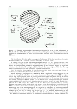
This chapter will give a description of the history how the BL Lac phenomenon was discovered and
studied. After that I will briefly describe the properties of BL Lac objects, the variability, radio and
optical properties and the environment in which BL Lacs are found. In Section 2.3 the different classes of
BL Lac objects will be introduced and the following section gives an overview about the different existing
models and unification schemes.
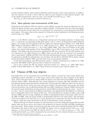
2.1 History of BL Lac astrophysics
The AGN class of BL Lac objects is named after the prototype BL Lacertae (J2000.0: 22h
02m
43.3s
+42d
16m
40s
). This variable object was found by Hoffmeister (1929) at the Sonneberg observatory in
Th¨uringen who classified it as a short period star of 13 − 15 magnitude and listed it as “363.1929 Lac”.
The name “BL Lacertae” was given by van Schewick (1941) at the Universit¨ats Sternwarte Berlin-
Babelsberg who searched on photographic plates which had been taken at the Sonneberg observatory
between December 1927 and September 1933. He found that BL Lacertae is an irregular variable star1
whose photographic magnitude varies between 13.5 mag and 15.1 mag.
Schmitt (1968) reported that the variable star BL Lacertae coincided with the radio source VRO 42.22.01.
This source showed linear polarization at 4.5 and 2.8 cm (MacLeod & Andrew 1968) and rapid variations
in the radio spectral flux (Biraud & V´eron 1968, Andrew et al. 1969, Gower 1969). A high polarization
of 9.8 % was also visible in the steep (Γ = −2.78) optical spectrum (Visvanathan 1969). The spectrum
of BL Lacertae seemed to follow a single power law but, different to other quasars, showed no emission
lines (Du Puy et al. 1969, Oke et al. 1969). Racine (1970) reported 0.1 mag variation over a few hours
in the optical and flicker of amplitude ∆V ≃ 0.03 mag with durations as short as ∆t = 2 minutes.
The next BL Lac objects to be identified, OJ 287 and PKS 0735+17, were also selected on the basis
of their unusual radio spectra (Blake 1970). Of course, at that time it was not clear whether BL Lac
objects are extragalactic sources or not.
Subsequent optical, infrared, and radio observations by several investigators led Strittmatter et al.
(1972) to suggest that objects similar to BL Lacertae comprise a class of quasi-stellar objects.
But due to the lack of emission and absorption lines it was not possible to determine the distance of
these variable objects. Pigg and Cohen (1971) tried to put constraints on the redshift by analyzing the
radio data of BL Lacertae, but could only give a lower limit of the distance (d > 200 pc). Finally Oke
and Gunn (1974) were able to determine the redshift of BL Lacertae by identifying absorption features in
spectra taken with the 5m Hale telescope between 1969 and 1973. They found the MgI line, the G-band
and the calcium-break and derived a redshift of z ≃ 0.07 (more accurate measurements show z = 0.0686).
They also determined the type of the host galaxy from the spectral energy distribution (SED) to be an
elliptical galaxy and suggested that the central source is similar to those in 3C 48, 3C 279, and 3C 345.
These objects have later been identified as a Sy1.5, a BL Lac object, and a Blazar respectively.
1van Schewick wrote: BL Lac. Unregelm¨aßig. Halbregelm¨aßiger Lichtwechsel zeitweise angedeutet, doch erlaubt das
geringe Beobachtungsmaterial keinen einwandfreien Schluß auf RV Tauri-Charakter. [...] Der Stern ist nicht rot.
13](https://image.slidesharecdn.com/6fabd339-d5aa-41a1-a40d-3283bf94795f-160804141441/85/doctor-13-320.jpg)

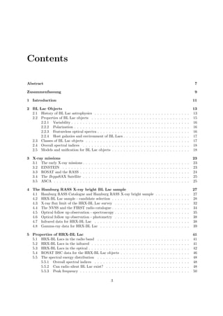
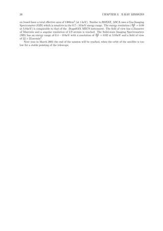
![24 CHAPTER 3. X-RAY MISSIONS
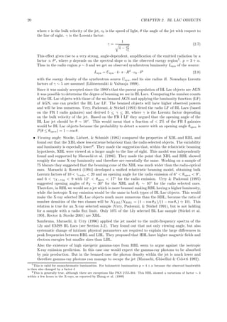
Figure 3.1: Missions in the X-ray and gamma range, which have been launched since 1990 (Graphic:
HEASARC).
3.3 ROSAT and the RASS
The X-ray selected sample of BL Lacs presented in this work is based on data taken with the ROSAT
satellite.
The focal plane of the X-ray telescope hosted the “Position Sensitive Proportional Counter” (PSPC,
Tr¨umper 1982) which detected photons in the 0.07–2.4 keV energy band. Compared to EINSTEIN,
ROSAT examined a significantly “softer” energy region. Thus it was possible to detect X-ray sources
with steeper and softer X-ray spectra. The PSPC detected the incoming photons in 240 energy channels.
Because of the low energy resolution (Brinkmann 1992),
∆E
E
=
0.415
√
E
(with E in keV) (3.1)
it is not possible to determine directly the photon energy from the channel, in which the photon has been
detected. It is only possible to have four independent “colors” within the PSPC energy band. The color
definition used in the optical astronomy is not useful for X-rays. Instead of colors, two hardness ratios
are defined by the following formula:
HR =
H − S
H + S
(3.2)
Herein H is the hard and S is the soft X-ray energy band. Hardness ratio 1 (HR1) is defined with S
being the number of photons within the channels 11–41 while H uses the hard channels 52–201. HR2 is
defined with S = [52 − 90] and H = [91 − 200]. Thus the hardness ratio is a measure for the hardness
of the detected X-ray radiation. It ranges by definition from -1 for extreme soft up to +1 for very hard
X-ray sources.
ROSAT was launched on June 1, in 1990 and saw first light on June 16, 1990 (Tr¨umper et al. 1991a).
The following six weeks were used for calibration and verification. End of July ROSAT started to do the
first complete X-ray survey of the entire sky with an imaging X-ray telescope. The “ROSAT All Sky
Survey” (RASS; Voges 1992) was performed while the satellite scanned the sky in great circles whose
planes were oriented roughly perpendicular to the solar direction. This resulted in an exposure time
varying between about 400 sec and 40,000 sec at the ecliptic equator and poles respectively. During the
passages through the auroral zones and the South Atlantic Anomaly the PSPC had been switched off,
leading to a decrease of exposure over parts of the sky. For exposure times larger than 50 seconds the sky
coverage is 99.7 %; a 97% completeness is reached for ≥ 100 seconds exposure time (Voges et al. 1999).A
secure detection of point sources is possible, when the count rate exceeds 0.05 sec−1
(Beckmann 1996).](https://image.slidesharecdn.com/6fabd339-d5aa-41a1-a40d-3283bf94795f-160804141441/85/doctor-24-320.jpg)
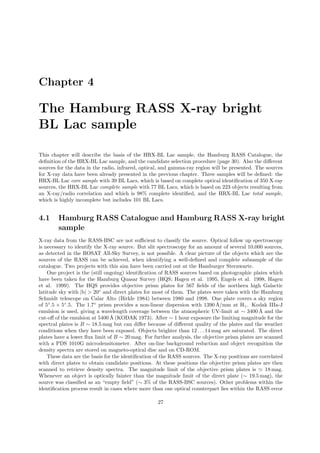
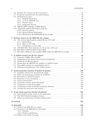
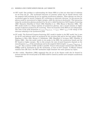
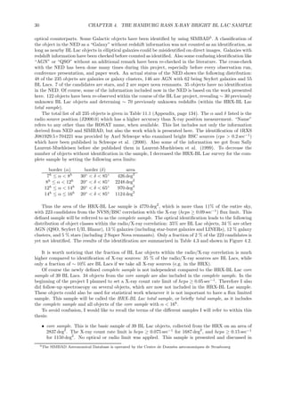
![4.2. HRX-BL LAC SAMPLE - CANDIDATE SELECTION 29
Table 4.1: Selection process for the HRX-BL Lac total and complete sample
selection number of objects comment
NVSS-BSC correlationa)
681 area: 5089 deg2
only objects with hcps ≥ 0.05 585 HRX-BL Lac total sample: 101 BL Lacs
only objects with hcps ≥ 0.09 235 95 % identified
decreased area to 4770 deg2
223 98 % identified (77 BL Lacs)
(HRX-BL Lac complete sample)
a)
flux-limits: fR(1.4 GHz) = 2.5 mJy, fX(0.1 − 2.4 keV) > 0.05 sec−1
Table 4.2: Properties of the Hamburg BL Lac samples in comparison to the RGB and EMSS sample
sample Reference number of X-ray radio optical
objects limit limit limit
HRX core sample Bade et al. 1998 39 0.075/0.15 sec−1 a)
- -
HRX-BL Lac total this work 101 0.05 sec−1 a)
2.5 mJyb)
-
HRX-BL Lac complete this work 77 0.09 sec−1 a)
2.5 mJyb)
-
RGB Laurent-Muehleisen 127 0.05 sec−1 c)
15 . . .24 mJyd)
18.5 mage)
RGB complete et al. 1999 33 0.05 sec−1 c)
15 . . .24 mJyd)
18.0 mage)
EMSS Rector & Stocke 2001 41 2 × 10⁻¹³ f)
- -
a)
ROSAT All Sky Survey count rate limit for the hard (0.5 − 2 keV) PSPC energy band.
b)
NVSS radio flux limit at 1.4 GHz
c)
RASS count rate limit for the whole (0.1 − 2.4 keV) PSPC energy band.
d)
GB catalog flux limit at 5 GHz
e)
O magnitude determined from POSS-I photographic plates
f)
EINSTEIN IPC (0.3 − 3.5 keV) flux limit in [ erg cm−2
sec−1
]](https://image.slidesharecdn.com/6fabd339-d5aa-41a1-a40d-3283bf94795f-160804141441/85/doctor-29-320.jpg)
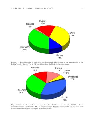
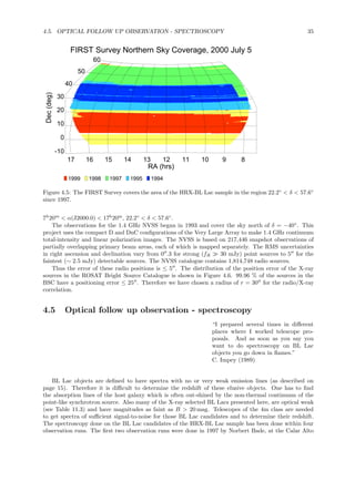
![4.5. OPTICAL FOLLOW UP OBSERVATION - SPECTROSCOPY 37
Table 4.5: Grisms used for spectroscopy with MOSCA at Calar Alto 3.5m telescope.
Grism coverage resolution
G500 4250 − 8400 ˚A 12 ˚A
R1000 5900 − 8000 ˚A 6 ˚A
G1000 4400 − 6600 ˚A 6 ˚A
The characterizing feature of BL Lac spectra in the optical is a non-thermal continuum which is
well described with a single power law. A second component is contributed by the host galaxy. If the
BL Lac itself shows no emission lines at all, it is only possible to determine the redshift of the object
by identifying absorption features of the host galaxy. The host galaxies are in majority giant elliptical
galaxies (e.g. Urry et al. 2000), as already described on page 17. These galaxies show strong absorption
features which are caused by the stellar content. Expected absorption features in the optical are an iron
feature at 3832 ˚A, the Ca H and K (3934 ˚A and 3968 ˚A, respectively), the G Band at 4300 ˚A, magnesium
at 5174 ˚A and the natrium D doublet at 5891 ˚A. A feature which is also prominent in most galaxy spectra
is the so-called “calcium break” at 4000 ˚A. When identifying candidates for the HRX-BL Lac sample,
the calcium break was used to distinguish between normal elliptical galaxies and BL Lac objects. The
calcium break is defined as follows (Dressler & Shectman 1987):
Ca − break[%] = 100 ·
fupper − flower
fupper
(4.2)
with fupper and flower being the mean fluxes measured in the 3750 ˚A < λ < 3950 ˚A and 4050 ˚A < λ <
4250 ˚A objects rest frame band respectively. In galaxies with a late stellar population, as expected in
elliptical galaxies, this contrast is about ≥ 40% with the higher flux to the red side of the break. Due to
low signal to noise within some spectra, the error of this value can be of the order of the measured break.
Nevertheless only a few objects within the HRX-BL Lac survey exhibit a calcium break in the range
25% < Ca − break < 40% (8 objects within the HRX-BL Lac total sample, and only 3 of the complete
sample). As will discussed later, these objects have also been included in the HRX-BL Lac total sample.
Objects with a calcium break > 40% have been identified as galaxies.
The interstellar medium can cause weak narrow emission lines in the spectrum, like the hydrogen
Balmer lines. In normal elliptical galaxies they are expected to be weak but can be seen in the most
powerful ellipticals, cD galaxies, with LINER properties. For higher redshifts, these features move out
of the optical wavelength region. Absorption lines from the interstellar gas become detectable. The
strongest lines are then the MgII doublet (2796.4 ˚A and 2803.5 ˚A, c.f. page 81), MgI 2853 ˚A, three FeII
lines (2382.8 ˚A, 2586.6 ˚A, and 2600.2 ˚A), and FeI 2484 ˚A. Expected equivalent widths are of the order
of several ˚A (Verner et al. 1994). A weak MnII line at 2576.9 ˚A might also be observable. These lines
can also be produced by intervening material and redshifts derived on this basis are lower limits rather
then firm values as derived from the lines produced by the stellar population. This is for example seen
in 0215+015 (Blades et al. 1985) with several absorbing systems in the line of sight.
Reliable redshifts can only be derived when more than one line is detectable. Some objects, like
PG 1437+398, do not show any absorption lines or other features, even in high signal to noise spectra
taken within several hours with telescopes of the 4m class. Also these objects are not necessarily optical
weak. PG 1437+398 for example has an optical magnitude of B ∼ 16 mag and is therefore one of the
brightest objects in the HRX-BL Lac sample.](https://image.slidesharecdn.com/6fabd339-d5aa-41a1-a40d-3283bf94795f-160804141441/85/doctor-37-320.jpg)
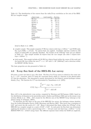
![4.8. GAMMA-RAY DATA FOR HRX-BL LAC 39
Table 4.6: HRX-BL Lac in the IRAS Faint Source Catalogue. Fluxes in mJy.
Name z F12µm F25µm F60µm F100µm log νLa
ν
RX J0721+7120 ? 112 126 237 783 45.2
RX J1419+5423 0.151 66 86 212 546 44.9
a
this value is constant for both objects within the IRAS energy region. For RX J0721+7120 a redshift
of z = 0.2 is assumed.
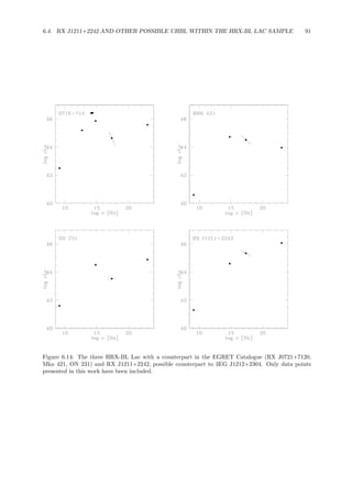
Table 4.7: HRX-BL Lac in the 3rd EGRET Catalogue
Name EGRET z F400MeV[pJy] log νLa
ν
RX J0721+7120 3EG J0721+7120 ? 29.8 ± 1.7 45.59
Mkn 421 3EG J1104+3809 0.030 24.5 ± 1.6 43.96
ON 231 3EG J1222+2841 0.102 20.2 ± 1.6 44.89
RX J1211+2242 ? 3EG J1212+2304 0.455 23.6 ± 6.4 46.07
a
applying α = 1 (Lin et al. 1992) at 1023
Hz (≃ 400 MeV). For RX J0721+7120 z = 0.2 is assumed.
the radio to the UV regime. These data are used to compute the log νLν values listed in table 4.6 and
are used for the further analysis of the spectral energy distribution.
In the near infrared the “Two-Micron All-Sky Survey” (2MASS, Skrutskie et al. 1995, Stiening et al.
1995) provides data for 52 objects of the HRX-BL Lac total sample (43 sources (57 %) of the complete
sample). The 2MASS is a survey of the sky using two ground based telescopes, one on the Mt. Hopkins
in Arizona and the other at the CTIO in Chile. Both telescopes are identical and are equipped with a
three channel camera, each channel consisting of a 256 × 256 HgCdTe detector. Thus at the same time
observations at three energy bands are possible; J (1.25µm), H (1.65µm) and Ks (2.17µm). Up to now
the survey covers 98.3% of the entire sky. Not all observations have already been analyzed. At the time of
writing, the 2MASS Second Incremental Release Point Source Catalog (2MASS-PSC) is available which
contains 160 million point sources. For extended sources an extra catalogue is constructed, the 2MASS
Second Incremental Release Extended Source Catalog (2MASS-XSC).
4.8 Gamma-ray data for HRX-BL Lac
A great fraction of the emitted radiation of BL Lac objects is set free in the high energy region beyond the
X-ray region. Therefore gamma-ray data are of high interest to the BL Lac community. The Energetic
Gamma-Ray Experiment Telescope (EGRET, Kanbach et al. 1988) on board the Compton Gamma Ray
Observatory (CGRO) covered the energy range between 20 MeV to over 30 GeV. EGRET worked for
nearly ten years before CGRO was safely de-orbited and re-entered the Earth’s atmosphere in June 2000
to avoid an uncontrolled re-entry in the atmosphere. The effective surface of the telescope was 0.15 m2
in
the 0.2–10 GeV region. The angular resolution was strongly energy dependent, with a 67 % confinement
angle of 5.5◦
at 100 MeV, falling to 0.5◦
at 5 GeV on axis; bright gamma-ray sources could be localized
with approximately 10 arcmin accuracy. The energy resolution of EGRET was 20 – 25 % over most
of its range of sensitivity. The data for the comparison with the HRX-BL Lac sample were taken from
the Third EGRET Catalogue (Hartman et al., 1999). This catalogue contains 271 gamma-ray sources
(E > 100 MeV) and includes data from 1991 detected April 22 to 1995 October 3.
Three of the HRX-BL Lac objects are included in the EGRET catalogue; the most relevant data are
listed in Table 4.7. The flux values at ∼ 1023
Hz are derived by multiplying the photon count-rates as
listed in the Third EGRET Catalogue with the conversion factors from Thompson et al. (1996). The
variation of the flux values is remarkable. I used only detections and no upper limits to derive the fluxes.
For computing fluxes I applied a weighted mean, based on the flux errors given in the EGRET catalogue.
Therefore the true minimal flux value could be even lower. One object of the HRX-BL Lac sample might
be a counterpart of the EGRET source 3EG J1212+2304. It is included in Table 4.7 and will be discussed
in the chapter about special single objects on page 89. The spectral energy distribution for these gamma](https://image.slidesharecdn.com/6fabd339-d5aa-41a1-a40d-3283bf94795f-160804141441/85/doctor-39-320.jpg)

![Chapter 5
Properties of HRX-BL Lac
In this chapter I will discuss the properties of the HRX-BL Lac sample in the different wavelength ranges
and also their spectral energy distribution. Whenever completeness is necessary to derive results, the 77
objects of the HRX-BL Lac complete sample are used. In cases, where the redshift information is needed,
only the 62 objects from the complete sample with known redshift are used.
Throughout this thesis luminosities are computed by
L = 4π · d2
l · fsource (5.1)
where fsource is the flux density in the source rest frame and dl is the luminosity distance. Assuming
a Friedmann universe (Λ = 0) the luminosity distance can be computed by the following formula (e. g.
Mattig 1958):
dl =
c0
H0 · q2
0
· [z · q0 + (q0 − 1) · ( (1 + 2q0z) − 1)] (5.2)
The proper distance, which is used to compute volumes in space, is related to the luminosity distance by
dl = dp · (1 + z).
Throughout this thesis I apply a Hubble parameter H0 = 50 km sec−1
Mpc−1
and a deceleration
parameter q0 = 0.5, assuming a Friedmann universe with Λ = 0.
5.1 HRX-BL Lacs in the radio band
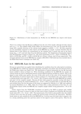
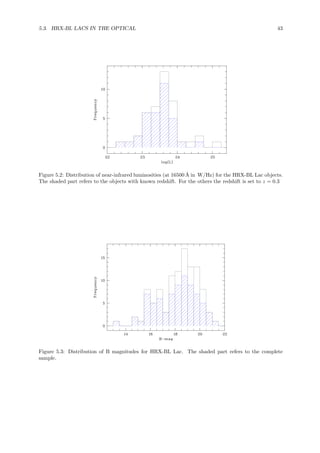
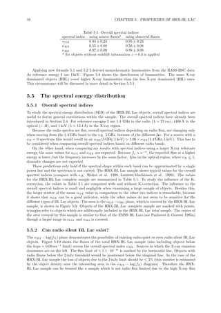
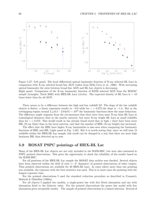
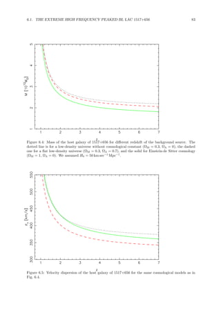
By definition all HRX-BL Lac objects are radio sources. The 1.4 GHz fluxes cover the range between
2.8 mJy of the faint end for the most distant object RX J1302+5056 (z = 0.688), and 768.5 mJy for
Markarian 421 (z = 0.03). The faintest BL Lac is MS 1019.0+5139 (Lr = 4.2 · 1023
W/Hz), the brightest
one is RX J0928+7447 (Lr = 1.3 · 1026
W/Hz, z = 0.638). Figure 5.1 shows the distribution of radio
luminosities for the HRX-BL Lac sample.
As expected for an X-ray selected sample, the radio luminosities are relatively low, thus still covering
a wide range. Applying the definition for radio-loudness (RL = log (fRadio/fB)) there is only one radio
quiet object (RL < 1), the BL Lac RX J1257+2412 (z = 0.141, fr,source = 13.2 mJy, B = 15.4 mag).
Thus, in principle, BL Lac objects seem to be radio loud objects, even when selected due to their X-ray
properties. The question whether if radio silent BL Lacs with RL ≪ 1 may exist will be discussed in
Section 5.5.1.
5.2 HRX-BL Lacs in the infrared
Only for one object (RX J0721+7120) in the HRX-BL Lac sample are IRAS infrared data available (see
table 4.6). This object shows a spectral slope of αIR ∼ 1 over the entire IRAS energy range.
For 52 HRX-BL Lacs data are available in the near infrared region (λ = 1 − 3 µm) from the 2MASS
survey as already described in Section 4.7. The mean value for the spectral slope in this regime is
α2 µm = 0.6 ± 0.2. Only one object (RX J1123+7230) shows an “inverse” spectrum with α2 µm = −1.1.
41](https://image.slidesharecdn.com/6fabd339-d5aa-41a1-a40d-3283bf94795f-160804141441/85/doctor-41-320.jpg)
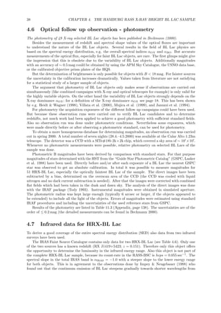
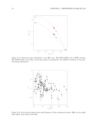
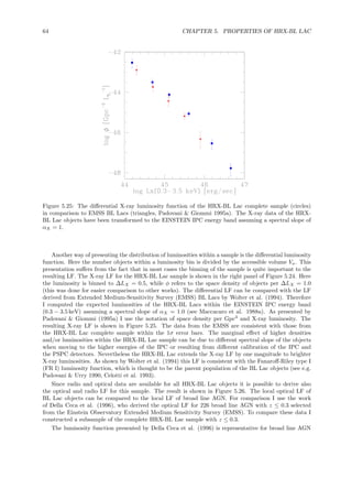
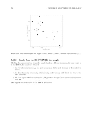
![44 CHAPTER 5. PROPERTIES OF HRX-BL LAC
Figure 5.4: Distribution of monochromatic optical luminosities in [ W/Hz] at λ = 4400 ˚A for the HRX-
BL Lacs with known redshift (applying αB−band = 0.6). The hashed area refers to the complete sample.
Figure 5.5: Distribution of calcium break values for the 30 BL Lac of the HRX-BL Lac total sample,
where it was possible to determine the break (the shaded region marks the complete sample). Negative
values can arise from a strong underlying non-thermal continuum.](https://image.slidesharecdn.com/6fabd339-d5aa-41a1-a40d-3283bf94795f-160804141441/85/doctor-44-320.jpg)
![46 CHAPTER 5. PROPERTIES OF HRX-BL LAC
5.4 ROSAT BSC data for the HRX-BL Lac objects
The sample of HRX-BL Lac objects is defined by the correlation of radio and X-ray sources. The X-ray
data are taken from the RASS-BSC (see Section 3.3). As described, the RASS data for most objects only
contain very few photons. It is not possible to derive real spectra from this database. But the spectral
slope can be determined using the hardness ratios provided by the BSC (see formula 3.2). In principle
two methods to do this are possible: the first one is to use the absorption due to Galactic hydrogen and a
given spectral slope to simulate a spectrum. With those two parameters it is then possible to determine
the conversion factors (formula 4.1) for the different bands which determine the hardness ratios (formula
3.2). Thus a grid of (HR1, HR2)(ΓX, NH,Galactic) is produced, where (HR1, HR2) is a pair of hardness
ratios, ΓX is the photon index1
which describes the X-ray spectrum. The second possibility is to fix the
spectral slope only and search for the best parameter combination of (HR1, HR2, NH). These methods
are described in detail by Schartel et al. (1992, 1994). It is obvious that the resulting errors of the
method based on free-fitted absorption (we will call these values αX,free and NH,free) are larger than in
the procedure where the absorption is fixed to the Galactic value (αX and NH,gal).
Using the latter method, we derive a mean spectral slope of αX = 1.09±0.31 from the ROSAT-PSPC
data. The energy indices cover a range −1.78 ≤ αX < +0.86. The values derived with a free fitted
NH are remarkably steeper: αX,free = 1.41 ± 0.60 (covered range −2.64 < αX,free ≤ +0.05). These
values of αX,free are in good agreement with previous studies of the spectral slope of BL Lac objects.
Maraschi et al. (1995) reported αX = 1.56 ± 0.43 for three pointed ROSAT observations on X-ray bright
BL Lacs, and Perlman et al. (1996) found αX = 1.20 ± 0.46 for the EMSS BL Lac sample (Morris et
al. 1991). Brinkmann et al. 1997 investigated ROSAT-PSPC spectra for 91 BL Lacs, also finding the
spectral slope being steeper for free fitted absorption (αX = 1.23 ± 0.06 and αX,free = 1.35 ± 0.11).
Another work on ROSAT-PSPC data by Comastri et al. (1995a) derived αX = 1.30 ± 0.25, but different
to Brinkmann et al. 1997 they did find the same spectral slope when fitting αX,free and NH at the same
time (αX,free = 1.26 ± 0.20). Bade et al. (1994) found a mean spectral slope of αX = 1.49 ± 0.17 for
10 new detected HBL, and Fink (1992) derived αX = 1.39 ± 0.07 for ten already known BL Lacs. More
recently Siebert et al. (1998) found a value of αX = 1.35 ± 0.55 for intermediate BL Lac objects.
The spectral slope of X-ray selected BL Lac objects is thus slightly flatter than the values found for
X-ray selected emission-line AGN (e.g. αX = 1.50±0.48, Walter & Fink 1993; αX = 1.42±0.44, Ciliegi &
Maccacaro 1996; αX = 1.53 ±0.42, Beckmann 1996). With the spectral slopes derived from the hardness
ratios and the count rates I determined the conversion factors and the fluxes of the HRX-BL Lac by
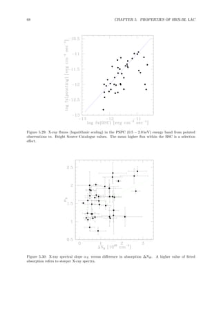
applying fx = CF · countrate (see page 32). The distribution of fluxes is shown in Figure 5.7. The sharp
cut-off at 10−12
erg cm−2
sec−1
is due to the count-rate limit of hcps ≥ 0.09 sec−1
. It is obvious that the
distribution of observed fluxes for HBL and IBL2
in the HRX-BL Lac is equivalent. The mean flux for the
HBL and IBL is (4.8±4.8)·10−12
erg cm−2
sec−1
and (7.1±18.6)·10−12
erg cm−2
sec−1
respectively. But
if we omit the bright source Mrk 421, we get for the IBL a mean flux of (4.2 ± 4.9) · 10−12
erg cm−2
sec−1
,
which is very similar to the value for the HBL.
For comparison of emission at different wavelengths, monochromatic fluxes are much more useful than
integrated fluxes. The formula of the monochromatic flux fE depends on the energy E0 at which the
monochromatic flux should be determined, on the energy band, defined by the energies E1 and E2, on
the spectral energy index αE, and on the integrated flux fx:
fE =
fx · (1 − αE)
E
(1−αE)
2 − E
(1−αE )
1
· E−αE
0 · (1 + z)αE−1
(5.3)
Here the last factor (1 + z)αE−1
is the K-correction term (see page 18). The flux is now in units
[ erg cm−2
sec−1
keV−1
]. Transformation of this flux value fE into µJy is done by applying
fE[ µJy] = fE[ erg cm−2
sec−1
keV−1
] ×
h · 1026
e
(5.4)
where h = 6.6262 · 10−34
J sec is the Planck constant, and e = 1.6022 · 10−19
C the electron charge.
1The energy index αE is related to the photon index Γ = αE + 1
2Here HBL are defined with αOX < 0.9 (log νpeak <∼ 16.4) and IBL have 0.9 ≤ αOX < 1.4 (16.4 <∼ log νpeak <∼ 14.6).](https://image.slidesharecdn.com/6fabd339-d5aa-41a1-a40d-3283bf94795f-160804141441/85/doctor-46-320.jpg)
![5.4. ROSAT BSC DATA FOR THE HRX-BL LAC OBJECTS 47
Figure 5.7: Distribution of the ROSAT-PSPC fluxes fx(0.5 − 2.0 keV) in [ erg cm−2
sec−1
] for the HRX-
BL Lac sample as derived from the Bright Source Catalogue. The shaded area marks the more X-
ray dominated objects (HBL) with αOX < 0.9. The strong X-ray source with fX(0.5 − 2.0 keV) =
1.2 · 10−10
erg cm−2
sec−1
is Markarian 421.
Figure 5.8: Distribution of monochromatic X-ray luminosities (LX(1 keV)[ W/Hz]) derived from the
ROSAT-BSC at 1 keV. The shaded area marks the more X-ray dominated objects with αOX < 0.9.](https://image.slidesharecdn.com/6fabd339-d5aa-41a1-a40d-3283bf94795f-160804141441/85/doctor-47-320.jpg)
![5.5. THE SPECTRAL ENERGY DISTRIBUTION 49
Figure 5.9: The αOX −αRO plane covered by the HRX-BL Lac objects. The points refer to the complete
sample, the triangles mark objects which are additionally included in the HRX-BL Lac total sample which
is not complete. Objects with αRO < 0.2 are called radio quiet.
Figure 5.10: X-ray flux (logarithmic scaling) in [ erg cm−2
sec−1
] versus αRX. X-ray loud objects are on
the left. The horizontal line marks the flux limit of the HRX-BL Lac complete sample, the diagonal line
refers to the 2 mJy limit of the NVSS.](https://image.slidesharecdn.com/6fabd339-d5aa-41a1-a40d-3283bf94795f-160804141441/85/doctor-49-320.jpg)
![52 CHAPTER 5. PROPERTIES OF HRX-BL LAC
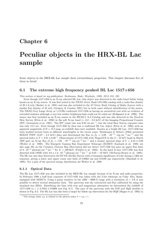
Figure 5.13: Distribution of difference in absorption ∆NH = NH,free − NH,gal for all HRX-BL Lac.
Shaded are the objects with errors σ∆NH < 3.5 · 1020
cm−2
.
Table 5.2: Difference in absorption
selection ∆NH[1020
cm−2
]a
∆NH[1020
cm−2
]
[1020
cm−2
]a
(all HRX-BL Lac) (HRX-BL Lac complete sample)
all objects 1.27 ± 1.93 (101) 1.00 ± 1.47 (77)
σNH < 3.5 1.27 ± 1.24 (48) 1.34 ± 1.23 (40)
pointed observationsb
1.11 ± 0.67 (40) 1.16 ± 0.71 (33)
a
in brackets the number of objects is given
b
see Section 5.9
positive and negative differences in absorption. The latter makes physically no sense so that the negative
values are probably due to the large uncertainties of the fit. This is supported by their disappearance
if the fits with largest errors (σNH > 3.5 · 1020
cm−2
) are omitted. This is demonstrated in Figure 5.13.
The resulting mean values are listed in Table 5.2. Here I also list the difference in absorption measured
in pointed observations as will be investigated in Section 5.9.
Therefore the result from the HRX-BL Lac sample is that when fitting a single power law with free
absorption to the ROSAT-PSPC data, the absorption is significantly higher than the Galactic value.
There are three possible explanations for the difference in absorption:
• intrinsic absorption: If matter within the BL Lac objects would cause the difference in absorption,
the same matter is expected to be heated and radiating thermal emission at lower (e.g. infrared)
energy regions. This is not seen: the spectrum of BL Lac objects is non-thermal throughout the
entire observed wavelengths. Also, intrinsic absorption should cause a negative correlation between
the luminosity and the ∆NH. A higher absorption should result in lower luminosities, although
this effect might not be detectable.
• absorption in the line of sight: Absorption in the line of sight with a mean column density of
∼ 1020
cm−2
is not expected in all observed cases. At least for the highest values of ∆NH this
should result in absorption lines seen in the optical spectra.
• absorption mimicked by the fit: The most plausible reason for the detected ∆NH could be a curvature
in the X-ray spectrum. Then a single-power law without additional absorption would not give a
sufficient fit, but an additional NH would effect the soft X-ray fit much more than the fit at higher](https://image.slidesharecdn.com/6fabd339-d5aa-41a1-a40d-3283bf94795f-160804141441/85/doctor-52-320.jpg)
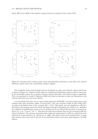
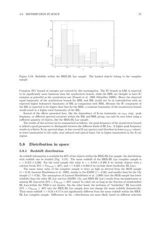
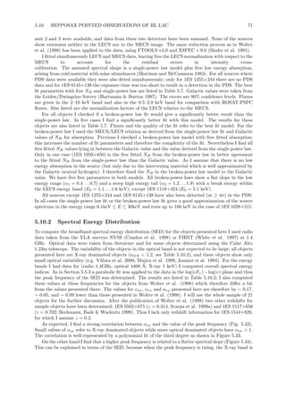
![5.7. PROPERTIES CORRELATED WITH THE PEAK FREQUENCY 55
αOX and αX respectively, than the HBL (marked in blue). The curvature of both objects is typical for
the HBL and IBL within the HRX-BL Lac sample. Here I fitted again a parabola. The curvature is
stronger in the SED of the IBL than in the HBL. This results in a higher ∆NH as explained above.
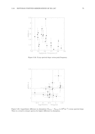
The differences in curvature can also be detected with the αXOX = αOX −αX value (Sambruna et al.
1996). This index describes the curvature between the X-ray spectrum and the overall spectral index αOX.
A negative value of αXOX stands for a steepening of the spectrum to higher energies (convex spectrum):
a positive value results from a concave spectrum. A correlation of αXOX and ∆NH for the HRX-BL Lac
sample can only be found when using the objects with errors in NH,free of σNH < 3.5 · 1020
cm−2
. Then
the correlation coefficient is rXY = 0.34 and the probability for an existing correlation is Γ > 95%. This
is consistent with the results from Sambruna et al. (1996) and Laurent-Muehleisen et al. (1999) who
report a correlation of X-ray dominance αOX and αRO.
Another correlation reported by those authors, αXOX vs. αRO, is not detectable in the HRX-BL Lac
sample. This might originate from the smaller range in αOX and αRO of objects (no BL Lacswith real
low peak frequencies like in the 1Jy sample) inside the HRX-BL Lac sample.
Figure 5.17: Monochromatic luminosities in the radio (1.4 GHz), near infrared (K-band), optical (B-
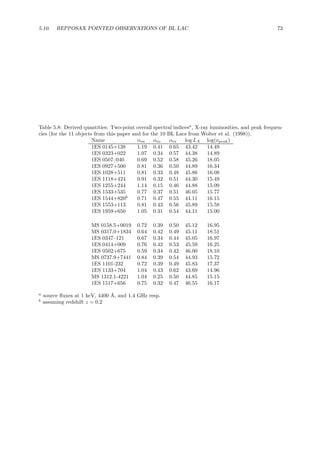
band), and X-ray (1 keV) regime versus peak frequency.
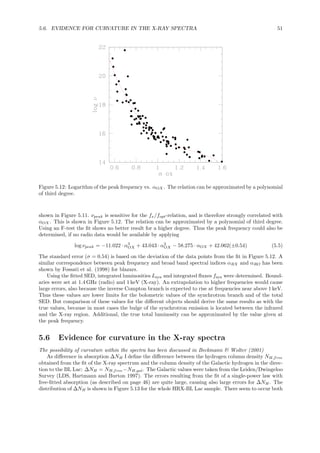
Another important set of physical parameters which are connected with the peak frequency are the
luminosities. The correlations with the monochromatic luminosities are presented in Figure 5.17. To
compute luminosities, the unknown redshifts were set to z = 0.3 which is the mean value for the HRX-
BL Lac sample. Luminosities are given in [ W/Hz]. The plots also show the linear regression. While in
the radio, near infrared, and optical region the luminosity is decreasing with increasing peak frequency,](https://image.slidesharecdn.com/6fabd339-d5aa-41a1-a40d-3283bf94795f-160804141441/85/doctor-55-320.jpg)
![56 CHAPTER 5. PROPERTIES OF HRX-BL LAC
Table 5.3: Connection of luminosity with peak frequency
region rxy Pearson probability linear regressiona
coefficient of correlation
radio (1.4 GHz) -0.23 > 97% log LR = −0.09 · log νpeak + 26.4
near IR (K-band) -0.28 > 95%b
log LK = −0.14 · log νpeak + 25.9
optical (B-band) -0.37 > 99.9% log LB = −0.13 · log νpeak + 25.1
X-ray (1 keV) +0.51 > 99.9% log LX = +0.19 · log νpeak + 17.3
total (radio – X-ray) -0.12 log Ltot = −0.04 · log νpeak + 22.0
a
Luminosities in [ W/Hz]
b
The lower probability results from the lower number of objects (52) with known K-band magnitudes.
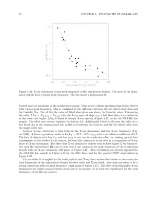
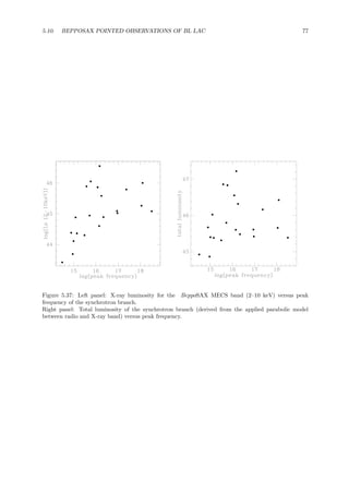
Figure 5.18: Left panel: The integrated luminosity. There seem to be no HBL with high luminosities
within the synchrotron branch.
Right panel: Data binned into ∆ log νpeak = 1. The data seem to be consistent with one mean Lsyn for
HBL and IBL.
the situation at X-ray energies is the other way around. In Table 5.3 there are more details listed to the
single regressions, including the probability of correlation.
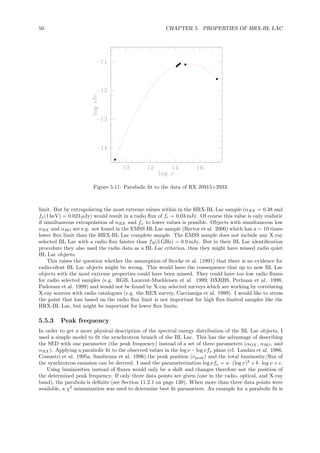
The total luminosity within the synchrotron branch has been derived as described on page 51 by
integrating the spectral energy distribution between the radio and the X-ray band. The relation of
peak frequency with the total luminosities does not show a clear correlation. Though a trend to lower
luminosities with increasing peak frequency can be seen in Figure 5.18, the significance of the correlation
is low due to the wide spread at the low frequency peak end. A problem of this correlation is also that a
peak frequency higher than 1 keV is outside the range of the computed integrated flux. Therefore I tried
different upper boundaries of the integration, but a correlation between total luminosity and νpeak is not
clearly measurable.
Also binning the data due to their peak frequencies does not show a correlation. For the right panel
of Figure 5.18 I used a binning of ∆ log νpeak = 1. The error bars refer to the logarithmic values of νpeak
and total luminosity L of the synchrotron branch. Within the errors the values are consistent with a
constant mean total luminosities over the whole range of measured peak frequencies.
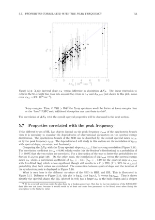
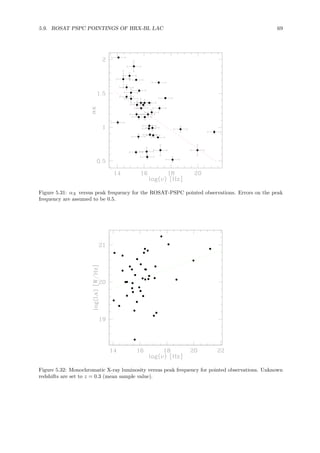
The non-detection of the correlation between luminosity and νpeak might be based on the fact that for
a fraction of ∼ 20% the redshift information is still missing. This leads to a lower statistic, if leaving these
objects out of the analysis, or to larger errors, when assuming a medium redshift for those objects. Based
on Figure 5.18 it can be at least said that there are no HBL with high luminosities (Lsyn ≫ 1022
W/Hz)
within the synchrotron branch.
Also I would like to stress the fact that the synchrotron branch is only part of the total emission of
the BL Lac objects. A large fraction and perhaps the majority of the emission is expected in the inverse](https://image.slidesharecdn.com/6fabd339-d5aa-41a1-a40d-3283bf94795f-160804141441/85/doctor-56-320.jpg)
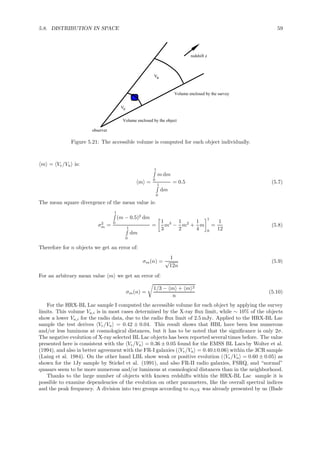
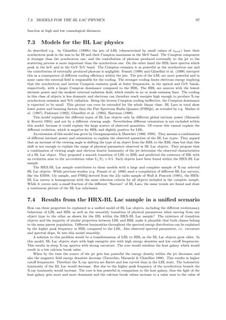
![58 CHAPTER 5. PROPERTIES OF HRX-BL LAC
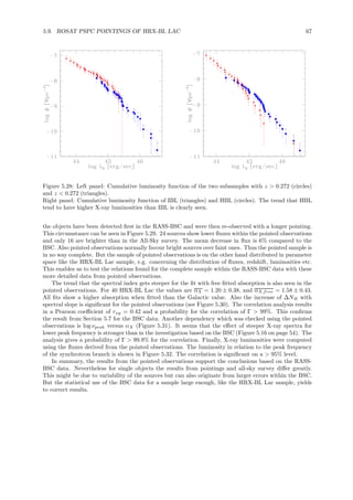
Figure 5.20: The redshift within the sample is increasing with higher peak frequency.
methods and therefore in different classes of BL Lac object, which are found in the surveys. The objects
within the HRX-BL Lac sample show a correlation of redshift with peak frequency (Figure 5.20). The
significance of the correlation is Γ > 99.9%. Therefore it could be possible that an X-ray selected sample
(like the EMSS or the HRX-BL Lac) shows higher redshifts than a radio selected one (like the RGB)
even though this might be a selection effect.
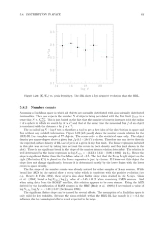
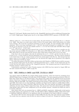
5.8.2 Ve/Va for HRX-BL Lac
A simple method to detect evolution in a complete sample of objects, is the application of a V/Vmax test
(Schmidt 1968). This test is based on the ratio of the redshift of the objects in relation to the maximal
allowed redshift zmax within the survey. If we have a sample of n objects, of which every object encloses
a volume Vi and this object would have been detected (due to the survey limit) up to a volume Vmax,i,
than the mean
V
Vmax
=
1
n
·
n
i=1
Vi
Vmax,i
(5.6)
will have a value in between the interval [0..1]. A value of V
Vmax
= 0.5 would refer to an equally
distributed sample in space. The area of the survey is not important for this value, because Vi/Vmax,i =
d3
p/d3
p,max with dp being the proper distance of the object redshift z and dp,max the value for zmax. This
test is very sensible to the maximal detected redshift zmax. Therefore Avni & Bahcall (1980) improved
the test by using Ve/Va (see Figure 5.21). Here Ve stands for the volume, which is enclosed by the object,
and Va is the accessible volume, in which the object could have been found (e.g. due to a flux limit of a
survey). Thus even different surveys with different flux limits in various energy bands can be combined
by the Ve/Va-test.
The error of Ve/Va can be determined as follows. For an equally distributed sample the mean value](https://image.slidesharecdn.com/6fabd339-d5aa-41a1-a40d-3283bf94795f-160804141441/85/doctor-58-320.jpg)
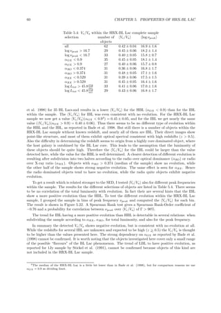
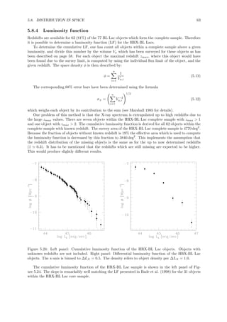
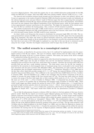
![62 CHAPTER 5. PROPERTIES OF HRX-BL LAC
-12 -11.5 -11 -10.5 -10
-3.5
-3
-2.5
-2
log fx [erg/cm**2/sec]
Figure 5.23: Left panel: Number counts for the HRX-BL Lac complete sample. The slope (−0.96 ± 0.05)
is determined by a linear regression.
Right panel: Number counts for the HBL (log νpeak > 16.4; circles) and for the LBL (marked by triangles).
The dotted line refers to a linear fit to the HBL data, the dashed line represents the LBL.
Another explanation would be a lack of low flux objects within the sample. But to achieve a value
of log N>fX / log fX = −1.5 the density of low-flux objects would have to be more than two times higher
than the value determined here. Even if there is a lack of low flux objects, it is not possible that it is that
high. On the other hand a misidentification of high flux objects could lead to a flattening of the number
counts relation. But also this is not expected, as the brighter objects are in most cases also easier to
identify than the apparently faint ones.
The flat slope might be more probably be caused by a lower space density of BL Lac objects at higher
redshifts (negative evolution). This would affect the high flux end less than the low flux end, resulting in
a slope flatter than the expected −1.5 for normally distributed objects. For the same reason the number
counts relation for quasars in the optical band shows a slope < −1.5 because these objects exhibit positive
evolution.
The turnover point near fX = 8 × 10⁻¹²
erg cm−2
sec−1
as reported in Bade et al. (1998) for the
39 BL Lacs of the HRX-BL Lac core sample is not confirmed by the investigation presented here. The
slope might be slightly steeper at fluxes higher than fX = 10−11
erg cm−2
sec−1
, but the statistically
significance at this level is low due to the small number of objects. On the other hand the objects with
fluxes below this value, which were found to have a slope of ≃ −0.5 for the core sample are clearly not
detected within the complete sample. Also, the turnover point around fX = 10−12
erg cm−2
sec−1
as
reported from EMSS data (Maccacaro et al. 1988b) cannot be verified here, because the turnover is
below the flux limit of the HRX-BL Lac sample.
A difference in the number counts relation for high and low frequency cut-off BL Lac objects within
the HRX-BL Lac complete sample is not seen (Fig. 5.23, right panel). The dotted and the dashed line
show the linear regression to the number counts of HBL and IBL, respectively. The regression derives
nearly the same function: log N>fX = −(12.9 ± 1.11) − (0.91 ± 0.09) · log fX for HBL (log νpeak > 16.4)
and log N>fX = −(13.1 ± 1.03) − (0.92 ± 0.09) · log fX for IBL with log νpeak < 16.4. Hence the slope is
the same in both cases and the straight line is shifted by ∼ 0.2 which could be caused by the fact that
the IBL are expected to have lower X-ray fluxes due to selection effects, although the shift is only of low
significance.](https://image.slidesharecdn.com/6fabd339-d5aa-41a1-a40d-3283bf94795f-160804141441/85/doctor-62-320.jpg)
![70 CHAPTER 5. PROPERTIES OF HRX-BL LAC
Table 5.5: The objects of the sample
Name R.A. (2000.0) Dec. Redshift
1ES 0145+138 01 48 29.8 +14 02 16 0.125
1ES 0323+022 03 26 13.9 +02 25 15 0.147
1ES 0507–040 05 09 38.2 –04 00 46 0.304
1ES 0927+500 09 30 37.6 +49 50 26 0.186
1ES 1028+511 10 31 18.5 +50 53 34 0.361
1ES 1118+424 11 20 48.0 +42 12 10 0.124
1ES 1255+244 12 57 31.9 +24 12 39 0.141
1ES 1533+535 15 35 00.7 +53 20 38 0.890a
1ES 1544+820 15 40 15.6 +81 55 04 ?
1ES 1553+113 15 55 43.2 +11 11 20 0.360
1ES 1959+650 20 00 00.0 +65 08 56 0.047
a
the redshift for 1ES 1533+535 needs confirmation (Bade et al. 1998)
Table 5.6: Journal of BeppoSAX observations
Name obs. date LECS LECS MECS MECS PDS PDS
[sec] net counts [sec] net counts [sec] net counts
1ES 0145+138 30-31/12/97 10576 73.0 ± 9.5 12443 78.7 ± 11.0 - -
1ES 0323+022 20/01/98 6093 201.6 ± 14.5 14408 607.4 ± 27.2 6845 256 ± 561
1ES 0507–040 11-12/02/99 9116 441.6 ± 21.5 20689 1460.2 ± 40.4 9094 1515 ± 633
1ES 0927+500 25/11/98 8436 568.4 ± 24.3 22712 1967.3 ± 46.5 10129 692 ± 571
1ES 1028+511 1-2/05/97 4552 737.9 ± 28.1 12622 2448.7 ± 50.2 9484 2763 ± 718
1ES 1118+424 1/5/97 6027 236.5 ± 15.6 9982 541.3 ± 24.1 8496 170 ± 147
1ES 1255+244 20/6/98 2484 297.1 ± 17.4 6910 1037.9 ± 33.1 - -
1ES 1533+535 13-14/02/99 8321 319.4 ± 18.5 26773 931.6 ± 35.5 4056 308 ± 285
1ES 1544+820 13/02/99 8043 170.7 ± 13.6 23249 510.8 ± 26.9 10414 780 ± 363
1ES 1553+113 5/02/98 4421 1179.5 ± 34.5 10618 2157.6 ± 47.3 4671 542 ± 363
1ES 1959+650 4-5/05/97 2252 423.2 ± 20.7 12389 3243.4 ± 57.6 7348 830 ± 516
5.10 BeppoSAX pointed observations of BL Lac
This section is also included in my publication Beckmann et al. 2002.
During the time of my PhD I had the chance to work at the Osservatorio Astronomico di Brera for a
total of nine months. There I worked with BeppoSAX data of BL Lac objects. This enabled me to test
the relations found based on ROSAT data with another sample and a different X-ray instrument.
The Slew Survey Sample covers the whole high Galactic latitude sky, while the EMSS has a lower
flux limit but only refers to an area of ∼ 800 deg2
. By selecting objects with fluxes FX(0.1 − 10 keV) ≥
10−11
erg cm−2
sec−1
in the Slew Survey and FX ≥ 4 × 10⁻¹²
erg cm−2
sec−1
in the EMSS, a sample has
been obtained that combines the advantage of a flux limited sample with a wide coverage of the parameter
space. The objects analyzed here are the second half of a sample, for which the first 10 objects have
been presented in Wolter et al. (1998). The 11 objects presented here (for positions and redshifts see
Tab. 5.5) have been observed between May 1997 and February 1999. The data have been preprocessed
at the BeppoSAX SDC (Science Data Center) and retrieved through the SDC archive. Table 5.6 shows
the journal of observations, including exposure times and net count-rates for the LECS, MECS, and PDS
detector.
5.10.1 Spectral analysis
The three MECS units spectra have been summed together to increase the S/N for data taken in May
1997. On May 6, 1997 a technical failure caused the switch off of unit 1. After this date, only MECS](https://image.slidesharecdn.com/6fabd339-d5aa-41a1-a40d-3283bf94795f-160804141441/85/doctor-70-320.jpg)
![72CHAPTER5.PROPERTIESOFHRX-BLLAC
Table 5.7: Best fit results for the BeppoSAX spectra. Single-power law with free fitted NH and, if the fit shows better results, broken-power law with
Galactic absorption
Name Energy α1 α2 E0 Na
H Na
H Fb
X Fc
X Nmd
χ2
ν(dof) Prob.
Index αX [keV] (Gal) (Fit)
0145+138 1.50 +0.94
−0.68 4.59 10.4 +27.6
−8.9 0.35 0.45 0.86 0.38 (3) 77%
0323+022 1.58 +0.23
−0.21 7.27 31.6 +14.6
−11.5 2.24 1.93 0.81 0.51 (27) 98%
0507–040 1.14 +0.12
−0.11 7.84 14.5 +7.8
−5.6 3.88 2.72 0.82 0.73 (69) 95%
0927+500 1.18 +0.09
−0.09 0.40 +0.18
−0.23 1.27 +0.08
−0.08 1.35 +0.28
−0.24 1.31 4.3 +1.3
−0.9 4.59 4.59 0.69 0.88 (61) 74%
1028+511 1.32 +0.08
−0.07 1.27 3.7 +0.8
−0.7 10.10 12.50 0.66 0.85 (97) 85%
1118+424 1.57 +0.16
−0.16 1.43 +0.08
−0.10 3.43 +0.7
−0.7 5.11 +1.6
−2.3 2.59 3.5 +1.3
−1.0 2.55 3.65 0.57 0.78 (23) 76%
1255+244 1.15 +0.12
−0.11 0.61 +0.19
−0.37 1.23 +0.13
−0.04 1.58 +0.36
−0.36 1.21 3.6 +1.5
−1.0 8.03 7.81 0.74 0.78 (36) 83%
1533+535 1.57 +0.15
−0.14 0.68 +0.19
−0.25 1.74 +0.16
−0.15 1.40 +0.30
−0.27 1.28 4.8 +1.9
−1.1 1.64 2.89 0.71 0.96 (44) 55%
1544+820 2.13 +0.29
−0.26 3.70 20.1 +11.3
−8.2 0.95 2.06 0.63 0.68 (30) 90%
1553+113 1.79 +0.09
−0.08 0.57 +0.18
−0.22 1.85 +0.09
−0.08 1.13 +0.90
−0.90 3.53 9.2 +2.3
−1.3 9.37 19.16 0.76 1.05 (89) 35%
1959+650 1.64 +0.08
−0.08 0.99 25.5 +7.1
−6.0 12.90 13.52 0.65 0.79 (88) 92%
a
hydrogen column density in ×1020
cm−2
b
unabsorbed flux in 10−12
erg cm−2
sec−1
in the 2–10 keV MECS energy band
c
LECS flux in the (0.5–2.0 keV) band in 10−12
erg cm−2
sec−1
d
Normalization of LECS versus MECS](https://image.slidesharecdn.com/6fabd339-d5aa-41a1-a40d-3283bf94795f-160804141441/85/doctor-72-320.jpg)

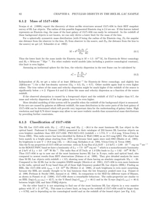
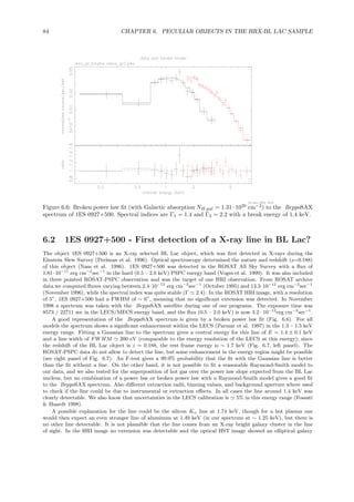
![80 CHAPTER 6. PECULIAR OBJECTS IN THE HRX-BL LAC SAMPLE
RX J1517.7+6525 z=0.702
4000 5000 6000
[Å]wavelength
0.70.80.91
Flux[10e−15erg/cm**2/sec]
FeII MgII
MgI
Figure 6.1: The spectrum of 1517+656, taken in February 1998 with the 3.5m telescope on Calar Alto,
Spain using the MOSCA spectrograph. The conditions during the exposure where not photometric, so
the flux values can only give a hint to the real flux. The curvature at the blue end below ∼ 4500˚A is due
to calibration problems. For the doublets see also Fig. 6.3
Table 6.1: Observed wavelengths and equivalent widths for absorption lines in the February 1998 spectrum
λobs[ ˚A] Wλ[ ˚A] λ0 [˚A] Ion Redshift
4194 0.03 2463.4 FeI 0.7025
- - 2484.0 FeI not detected
4404 0.15 2586.7 FeII 0.7026
4429 0.17 2600.2 FeII 0.7033
4761 0.48 2796.4 MgII 0.7025
4774 0.52 2803.5 MgII 0.7028
4855 0.15 2853.0 MgI 0.7017
4999 0.09 2937.8 FeI 0.7016
1993, because it had no published identification then and was independently found by the quasar selection of the
HQS. The 2700 sec exposure, taken with the 2.2m telescope on Calar Alto and Boller & Chivens spectrograph,
showed a power-law like continuum; the significance of the absorption lines in the spectrum was not clear due to
the moderate resolution of ≃ 10 ˚A (Fig. 6.2). Nevertheless the MgII doublet at 4761 and 4774˚A is also detected
in the 1993 spectrum, though only marginally resolved (see Table 2). The equivalent width of the doublet is
comparable in both images (W˚A
= 0.8/0.9 for the 1993/1998 spectrum respectively). Also the Fe II absorption
doublet at 4403/4228 ˚A (λrest = 2586.6/2600.2 ˚A) and Mg I at 4859 ˚A (λrest = 2853.0 ˚A) is detectable. For a
list of the detected lines, see Table 1. Comparison with equivalent widths of absorption lines in known elliptical
galaxies is difficult because of the underlying non-thermal continuum of the BL Lac jet. But the relative line
strengths in the FeII and MgII doublet are comparable to those measured in other absorption systems detected
in BL Lac objects (e.g. 0215+015, Blades et al. 1985). Because no emission lines are present and the redshift
is measured using absorption lines, the redshift could belong to an absorbing system in the line of sight, as e.g.
detected in the absorption line systems in the spectrum of 0215+015 (Bergeron & D’Odorico 1986). A higher
redshift would make 1517+656 even more luminous; we will consider this case in the further discussion, though
we assume that the absorption is caused by the host galaxy of the BL Lac. Assuming a single power law spectrum
with fν ∝ ν−αo
the spectral slope in the 4700 − 6600 ˚A band can be described by αo = 0.86 ± 0.07. The high
redshift of this object is even highly plausible, because it was not possible to resolve its host galaxy on HST snap
shot exposures (Scarpa et al. 1999a). The apparent magnitude varies slightly through the different epochs, having
reached the faintest value of R = 15.9 mag and B = 16.6 mag in February 1999 (direct imaging with Calar Alto
3.5m and MOSCA). These values were derived by comparison with photometric standard stars in the field of view
(Villata et al. 1998). H0 = 50 km sec−1
Mpc−1
and q0 = 0.5 leads to an absolute optical magnitude of at least
MR = −27.2 mag and MB ≤ −26.4 (including K-correction).](https://image.slidesharecdn.com/6fabd339-d5aa-41a1-a40d-3283bf94795f-160804141441/85/doctor-80-320.jpg)
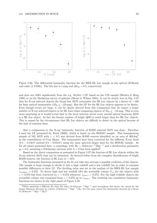
![6.1. THE EXTREME HIGH FREQUENCY PEAKED BL LAC 1517+656 81
HS 1517+6536 z=0.702
4000 5000 6000
[Å]wavelength
121620
Flux[10e−16erg/cm**2/sec]
FeII
FeI FeII MgII
MgI
Figure 6.2: The spectrum of 1517+656, taken with the 2.2m telescope on Calar Alto in August 1993.
Observation conditions were not photometric.
Table 6.2: Observed wavelengths and equivalent widths for absorption lines in the 1993 spectrum
λobs[˚A] Wλ[˚A] λ0 [˚A] Ion Redshift
4194 0.2 2463.4 FeI 0.7025
4231 0.1 2484.0 FeI 0.7033
4401 0.3 2586.7 FeII 0.7014
4429 0.4 2600.2 FeII 0.7033
4761 0.4 2796.4 MgII 0.7025
4771 0.4 2803.5 MgII 0.7018
4855 0.15 2853.0 MgI 0.7017
- - 2937.8 FeI not detected
RX J1517.7+6525 z=0.702
4400 4500 4600 4700 4800
[Å]wavelength
0.91
Flux[10e−15erg/cm**2/sec]
FeII
FeII
MgII MgI
Figure 6.3: Detail of the February 1998 spectrum with the FeII and MgII doublets.](https://image.slidesharecdn.com/6fabd339-d5aa-41a1-a40d-3283bf94795f-160804141441/85/doctor-81-320.jpg)
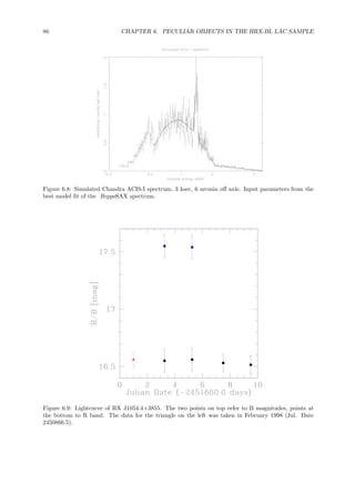
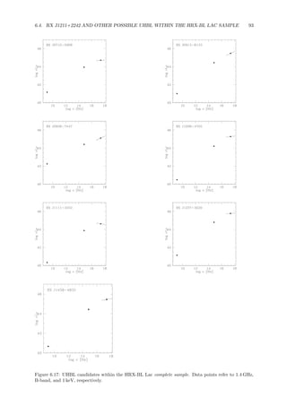
![6.3. RX J1054.4+3855 AND RX J1153.4+3617 87
RX J1054.5+3855, CA 3.5m, grism G500, 21/02/98 z=0.0
4500 5000 5500 6000 6500 7000 7500
wavelength [Å]
0.20.40.60.81
flux[10erg/cm²/sec/Å]−15
G−Band Hβ Mg+MgH NaI−D Hα
Figure 6.10: The spectrum of RX J1054.4+3855, observed in February 1998 at the Calar Alto 3.5m
telescope (20 min exposure). The line is at ∼ 6650˚A.
RX J1153+3617, CA 3.5m, grism G500, 22/02/98 z=0.0
4400 4800 5200 5600 6000 6400 6800
wavelength [Å]
1.522.533.54
flux[10erg/cm²/sec/Å]−16
G−Band Hβ Mg+MgH NaI−D Hα
Figure 6.11: The spectrum of RX J1153.4+3617, observed in February 1998 at the Calar Alto 3.5m
telescope (30 min exposure). The strong emission line is located at 6610˚A
.](https://image.slidesharecdn.com/6fabd339-d5aa-41a1-a40d-3283bf94795f-160804141441/85/doctor-87-320.jpg)
![88 CHAPTER 6. PECULIAR OBJECTS IN THE HRX-BL LAC SAMPLE
RXJ1153.4+3617, CA 2.2m, grism B100, 13/03/00 z=0.0
4000 4400 4800 5200 5600 6000
wavelength [Å]
0.511.522.533.5
flux[10erg/cm²/sec/Å]−14
Fe
CaH
CaK G−Band Hβ Mg+MgH NaI−D
Figure 6.12: The spectrum of RX J1153.4+3617, observed in March 2000 at the Calar Alto 2.2m telescope.
The breaks in the continuum are less significant.
Table 6.3: Properties of RX J1054.4+3855 and RX J1153.4+3617
Object hcpsa
fxb
frc
B-mag J-mag H-mag K-mag
RX J1054.4+3855 0.061 7.20 6.17 17.55 16.2 15.9 15.6
RX J1153.4+3617 0.060 7.15 6.10 17.51 - - -
a
ROSAT-PSPC “hard” (0.5 − 2 keV) countrate [sec−1
]
b
X-ray flux in 10−13
erg cm−2
sec−1
c
Radio flux at 1.4 GHz in mJy
the exposures are less good than for the February 1998 observation, the line and the break are still visible. The
second break at ∼ 4840 ˚A is not clearly detectable. The redshift of both objects remains uncertain. If the
redshift would be z ≃ 0.35, the line would be Hβ and the break at 6610˚A would refer to the calcium break. But
then also MgII should be clearly detectable at ∼ 3780 ˚A.
If the detected line would be MgII, the redshift of both objects would be z ≃ 1.35 and the properties in optical,
radio, and X-rays would support the identification as a BL Lac objects. But in this case, both objects would lie
far out of the common distributions of BL Lac objects, i.e. in a log LX vs. αOX diagram. On the other hand the
spectrum is similar to this of HE 1258–0823, a quasar at redshift z = 1.15 with weak MgII and only marginally
detected CIII line (Reimers, K¨ohler and Wisotzki 1996). Also the breaks in the continuum can be seen at the same
rest frame wavelengths (see also HE 0950–0852). Nevertheless this would seems to be implausible. The whole
NVSS/BSC correlation does include only one object at redshift z > 0.9, the blazar 0836+710 at z = 2.172 (see
Table 11.1). Therefore, these two objects would exhibit exactly the same properties while being clearly separated
(∆Position ∼ 5◦
).
An intensive optical monitoring campaign is planned for spring 2001 with the Hamburg 1.2m Oskar L¨uhning
telescope. If the objects are interacting binaries, they could show periodicity within their light curve on short
timescales.
More recent observations have confirmed the high-redshift nature of the two objects, with RX J1054.4+3855
being at z = 1.363 (White et al. 2000) and RX J1153.4+3617 at z = 1.358 (Schneider et al. 2007).](https://image.slidesharecdn.com/6fabd339-d5aa-41a1-a40d-3283bf94795f-160804141441/85/doctor-88-320.jpg)
![6.4. RX J1211+2242 AND OTHER POSSIBLE UHBL WITHIN THE HRX-BL LAC SAMPLE 89
RX J1153.4+3617, CA 2.2m, grism G100, 13/03/00 z=0.0
4500 5000 5500 6000 6500 7000 7500 8000
wavelength [Å]
1234
flux[10erg/cm²/sec/Å]−15
Hβ Mg+MgH NaI−D Hα
Figure 6.13: RX J1153.4+3617 observed with grism G100. The break at 5460 ˚A and the line at 6610 ˚A
are still existing.
Table 6.4: Sources (except normal galaxies) within the 3EG J1212+23 error circle as derived from the
NED
Name α δ Distance [arcmin] Type
3EG J1212+23 12 12 36 +23 04 48 0 Gamma-ray source
RX J1211+2242 12 11 59 +22 42 32 24 BL Lac object
ROSE 11 12 12 56 +22 35 19 30 Comp. Gal. Group
RX J1212+2232 12 12 06 +22 32 07 33 unidentified X-ray Source
Abell 1494 12 13 14 +23 56 19 52 Galaxy Cluster
6.4 RX J1211+2242 and other possible UHBL within the HRX-
BL Lac sample
A detailed study of RX J1211+2242 has been published in Beckmann et al. (2004).
Within the 95% confidence radius (53 arcmin) of the EGRET object 3EG J1212+2304 there is the HRX-
BL Lac RX J1211+2242 at a distance of 24 arc-minutes to the gamma-ray source. This BL Lac could be the
counterpart to the gamma-ray source. The redshift of this HBL is z = 0.455 as derived from absorption lines
within the optical spectrum (see Figure 6.16). Checking the NED I found 134 objects inside the 53 arcmin
circle. Most of them (130) are normal galaxies which should not produce any detectable gamma-ray emission.
Other identifications are listed in Table 6.4. From this list only the source RX J1212+2232, which is up to now
unidentified, could be a possible gamma bright counterpart. The galaxy cluster and also the compact group could
produce thermal X-ray emission up to a few keV but cannot be a relevant gamma-ray source. Figure 6.14 shows
the spectral energy distribution for the three HRX-BL Lacs which are also EGRET sources (see Table 4.7 on
page 39), and for the possible counterpart of 3EG J1212+2304. Only the data discussed here are included in this
graphic. A more detailed SED for MRK 421 can be found in Maraschi et al. (1999), the SED of 0716+714 is
described by Kubo et al. (1998). Compared to the spectral energy distribution of the other objects it is possible
that RX J1211+2242 is the true counterpart of the gamma-ray source. The gamma-ray point seems to be the
continuation of the SED from the radio to the X-ray region. It is worth noticing that the spectral slope in the
X-rays is only based on RASS data and therefore might be wrong. The errors shown for the slope result from
the fit to the hardness ratios only and might be significantly larger and even a flat X-ray spectral slope might be
possible. In this case RX J1211+2242 could be one of the Ultra High Frequency Peaked BL Lacs (UHBL), which
were first assumed to exist by Ghisellini (1999b). This assumption is based on the work of Guilbert, Fabian &](https://image.slidesharecdn.com/6fabd339-d5aa-41a1-a40d-3283bf94795f-160804141441/85/doctor-89-320.jpg)
![90 CHAPTER 6. PECULIAR OBJECTS IN THE HRX-BL LAC SAMPLE
Table 6.5: UHBL candidates within the HRX-BL Lac complete sample
Name z fR[ mJy] B[ mag] fa
X αX Fermi/LAT detection
RX J0710.5+5908 0.125 159 18.4 10.2 0.93 yes
RX J0913.3+8133 0.639 4.9 20.7 2.3 0.65 no
RX J0928.0+7447 0.638 85.8 20.8 1.1 0.66b
no
RX J1008.1+4705 0.343 4.7 19.9 4.4 0.93b
no
RX J1111.5+3452 0.212 8.4 19.7 2.7 1.13 yes
RX J1237.1+3020 0.700 5.6 20.0 3.2 0.94 no
RX J1458.4+4832 0.539 3.1 20.4 2.7 0.88 no
a
PSPC flux (0.5 − 2.0 keV) in [10−12
erg cm−2
sec−1
]
b
PSPC spectral slope derived from pointed observation
Rees (1983) who derived a limit on the maximum synchrotron frequency that can be reached by shock-accelerated
electrons. They draw the conclusion that νpeak,max ≃ 70 MeV, independent on the applied magnetic field strength
B. Finally Ghisellini suggests that ∼ 1 MeV can be considered a limit for the observed maximum frequency in
BL Lac objects. This value is certainly much lower than the frequency at which the EGRET observations have
been made (∼ 300 MeV). Nevertheless the restriction to this lower value by Ghisellini is based on the following
formula:
νpeak = 0.36 ·
R16Γ1
γ2
min(L′
s,42)3/2
MeV (6.3)
Here R16 is the cross sectional radius of the jet (in units 1016
cm), Γ1 the bulk Lorentz factor of the jet, and
L′
s,42 is the synchrotron intrinsic power (in units 1042
erg sec−1
). This can result in peak frequencies as high as
νpeak ∼ 1022
Hz, as has been demonstrated by Ghisellini (1999a).
Two objects of this class, which have the peak of the synchrotron branch at frequencies νpeak ≥ 1019
Hz, are
claimed to have been found. The first one is 1ES 1426+428, a BL Lac which is also included in the HRX-BL Lac
complete sample. This blazar peaks near or above 100 keV (Costamante et al. 2001). A second UHBL has been
found by Giommi et al. (2001). This object is 1RXS J123511.1-14033 and is thought to be the X-ray counterpart
of the EGRET gamma-ray source 2EG J1233-1407. The spectral energy distribution (Fig. 6.15) is very similar
to that of RX J1211+2242. All information gathered together makes it possible that RX J1211+2242 is indeed
the counterpart to the EGRET source 3EG J1212+2304. A follow-up observation at ∼ 1020
Hz could clarify, if
the BL Lac has continuous slope between the ROSAT-PSPC and the EGRET data point, or if there is the gap
between the synchrotron and the inverse Compton branch. Therefore an observation with the SPI spectrograph
on-board the INTEGRAL satellite (Pace, Pawlak, & Winkler 1994; Winkler 1999) is planed.
Besides RX J1211+2242 there are seven more objects within the HRX-BL Lac complete sample which show
peak frequencies above 1019
Hz. These objects are also promising targets for the INTEGRAL mission, although
the expected fluxes in the gamma-ray region might be low. The spectral energy distribution for these objects
is shown in Figure 6.17. Details to these objects can be found in Table 6.5. It is worth mentioning that the
determined peak frequency is based on non-simultaneous data. Therefore it is possible that the peak frequency
determined by the parabolic fit is wrong. Nevertheless the high frequency peaked objects are not expected to
vary a lot. The spectral slope in the X-rays was determined from the PSPC pointed observations in the cases of
RX J0928.0+7447 and RX J1008.1+4705. For the other objects the αX results from the hardness ratios within
the RASS. Although in these cases the errors on the photon index are large, the determined slope can give a hint
to the real value.](https://image.slidesharecdn.com/6fabd339-d5aa-41a1-a40d-3283bf94795f-160804141441/85/doctor-90-320.jpg)
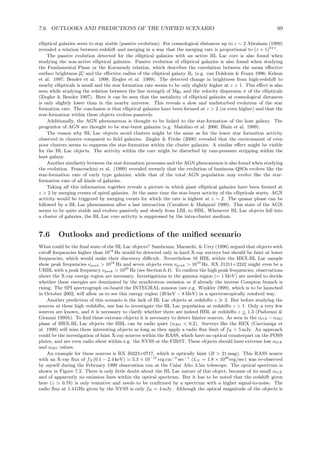
![92 CHAPTER 6. PECULIAR OBJECTS IN THE HRX-BL LAC SAMPLE
FIGURE 3. Left: the ROSAT and NVSS error circles showing the candidate UHBL
1RXS J123511.1-14033. Right: the SED of 1RXS J123511.1-14033 if this BL Lac is
the correct counterpart of the EGRET source 2EGJ1233-1407
that the synchrotron emission could reach the gamma ray band. A rst BeppoSAX
pointing of this object unfortunately gave inconclusive results since the observation
had to be split into three short exposures and the spectrum appears to be variable.
Details will be published elsewhere. A second UHBL candidate will be observed by
BeppoSAX in a few months. If these observations will con rm the hypothesis that
UHBLs exist, this type of sources could be the long sought counterpart of many of
the still unidenti ed high galactic latitude EGRET sources.
REFERENCES
Aller M.F, Aller H.D., Huges P.A., & Latimer G.E., 1999 ApJ 512, 601
Boella G. et al. 1997 A&AS, 122, 299
Chiappetti,L., et al. 1999, ApJ 521, 552
Ghisellini, G., 1999, Proc 3rd Integral Workshop, Taormina, astro-ph/9812419
Giommi P.,& Fiore F. 1998, in Proc. 5th Workshop on Data Analysis in Astronomy, World Scien-
ti c, Singapore, p. 93
Giommi, P., Padovani, P. & Perlman, E. 1999, MNRAS in press, astro-ph/9907377
Giommi, P. et al. 1999, A&A, in press, astro-ph/9909241
Giommi, P., Menna, M.T., & Padovani, P. 1999, MNRAS in press, astro-ph/9907014
Kollgaard R.I., 1994 Vistas in Astronomy, 38, 29
Padovani, P. & Giommi, P. 1995, ApJ, 444, 567
Padovani, P. et al. 1999, in preparation
Pian, E. et al. 1998, APJ L,492, L17
Tagliaferri, G., et al. 1999, A&A, submitted
Urry, C.M., & Padovani, P., 1995, PASP, 107, 803
Wolter, A. et al. 1998 A&A 335, 899
4
Figure 6.15: The spectral energy distribution of the UHBL 1RXS J123511.1-14033 (as presented by
Giommi et al. 2001).
RXJ 1211.9+2242 G500 z=0.455
4400 4800 5200 5600 6000 6400 6800
wavelength [Å]
00.40.81.21.6
flux[10erg/cm²/sec/Å]−16
Fe
Ca H+K
G−Band
Figure 6.16: Optical spectrum of RX J1211+2242 taken with Calar Alto 3.5m / MOSCA.](https://image.slidesharecdn.com/6fabd339-d5aa-41a1-a40d-3283bf94795f-160804141441/85/doctor-92-320.jpg)

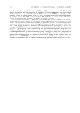
![102 CHAPTER 7. A UNIFIED SCENARIO FOR BL LAC OBJECTS
RX J0323+0717, CA3.5m, MOSCA, G500 z=0.783 ?
5000 6000 7000 8000 9000
wavelength [Å]
01234
flux[10erg/cm²/sec/Å]−17
MgII
MgI
Fe
Ca H+K
G−Band Hβ
Figure 7.2: The X-ray dominated object RX J0323+0717, observed with MOSCA at the Calar Alto 3.5m
telescope in February 1999. The redshift of z ≃ 0.783 is tentative.](https://image.slidesharecdn.com/6fabd339-d5aa-41a1-a40d-3283bf94795f-160804141441/85/doctor-102-320.jpg)
![8.1. CANDIDATE SELECTION FOR THE SEYFERT II SAMPLE 105
• 13.0 mag < spcmag < 17.0 mag1
• Effective radius on the direct plate > 64 pixel
• No narrow lines in the range 4103 . . . 4774 ˚A and 3639 . . . 3773 ˚A. In this interval no narrow lines are expected
• No narrow lines blue-wards of 3346 ˚A
• No broad emission lines with 3960 ˚A < λ < 4902 ˚A
• No broad emission lines blue-wards of 3773 ˚A
• In addition I used a color criterion, to reject normal galaxies. For Seyfert II galaxy candidates the colors
had to be in the range 1550 < xhpp1 < 2314 and 650 < xhpp2 < 1150
• Objects which showed calcium H and K lines, but were not “red enough”, were rejected by the candidate
selection.
The selection of Seyfert II candidates from objects without detectable emission lines was done by applying
the following criteria:
• Spectrum does not include an overlap
• Effective radius on the direct plate > 120 pixel2
• 13.0 mag < spcmag < 17.0 mag
• Additionally a color selection was used which was optimized for the learning sample3
Seyfert II candidates found by this selection procedure were then checked for counterparts in the NASA/IPAC
Extragalactic Database (NED)4
. The information from the NED was used in the following way:
An object classified as a galaxy without redshift information was still taken as a Seyfert II candidate. Only
objects with a secure classification and redshift were counted as “identified”. If there were any doubts due to
extreme density spectra, those objects were still included in the candidate procedure. The fraction of objects
which could be clearly identified with the information from the literature and from the NED was ∼ 30%, strongly
depending on the field. Objects which had been classified as Seyfert II galaxies were included into the Seyfert II
sample.
The reduced list of candidates was then checked one by one. A major fraction of the selected candidates were
obvious stars: often the automatic line detection algorithm mis-identified the absorption doublet of calcium at
3933/3968 ˚A as an emission line. Furthermore, when possible, the redshift of the candidates was estimated using
the detected lines. Candidates which clearly showed a redshift z ≫ 0.07 were sorted out.
The remaining candidates were sorted interactively into categories of the likelihood of Seyfert II nature of the
object. Chosen categories were:
1 – candidate with several clear Seyfert II characteristics, like strong [OII]3727 ˚A line, [NeV]3426 ˚A emission or
[OIII]5007 ˚A line.
2 – candidate with one Seyfert II characteristic. At least one of the criteria of (1) should be fulfilled.
3 – candidate for which it is not impossible to be a Seyfert II galaxy.
Using this semi-automatic procedure, in total 67 ESO fields have been worked through. Of ∼ 700, 000 overlap
free density spectra, the semi-automatic procedure selected ∼ 1, 700 candidates which were all cross checked with
the NED. After the final selection, 393 candidates were left over, which are distributed into the different categories
as follows:
candidate class 1: 21 objects
candidate class 2: 87 objects
candidate class 3: 285 objects
Figure 8.2 shows an example of a density spectrum of a Seyfert II candidate. This candidate has been selected
due to line criteria from the point-like sources in the HES data base. The [OIII]5007 ˚A line is clearly visible on
the red (left) end of the spectrum. The slit spectrum of this object is presented in Figure 8.4. For comparison
Figure 8.3 shows a color selected candidate. No lines are detected within the density spectrum and the selection
is based on color criteria only. Also this object turned out to be a Seyfert II galaxy with a weak active core within
a relatively bright galaxy.
1Here 17 mag is the lower flux limit. The upper limit of 13 mag was chosen to reject bright stars, which are often
mis-identified as galaxies because of there large apparent extension on the direct plates.
2The selection based on colors only is very difficult, therefore it was necessary to apply a more strict extension criterion
than for the line-based sample
3exact criterion for Seyfert II color based selection: 1550 < x hpp1 < 2314, 650 < x hpp2 < 1150, and 1350 < xqd < 2382
4The NED is operated by the Jet Propulsion Laboratory, California Institute of Technology, under contract with the
National Aeronautics and Space Administration.](https://image.slidesharecdn.com/6fabd339-d5aa-41a1-a40d-3283bf94795f-160804141441/85/doctor-105-320.jpg)

![8.2. FOLLOW-UP SPECTROSCOPY OF SEYFERT II CANDIDATES 107
HE 0201−3029 slit spectrum z=0.036
5200 5600 6000 6400 6800
510152025
flux[10erg/cm²/sec/Å]−16
30
wavelength [Å]
He Hβ
OIII]
MgI NaI OI [NII]
HHα
[SII]
Figure 8.4: Slit spectrum of HE 0201-3029 taken with the Danish 1.54m telescope using DFOSC in
December 1999. The slit spectrum reveals the Seyfert II properties of this object.
8.2 Follow-up spectroscopy of Seyfert II candidates
To determine the true object type of the candidates, follow up spectroscopy was necessary. Two observation
runs were done at the Danish 1.54m telescope on La Silla, using the Danish Faint Object Spectrograph and
Camera (DFOSC). The first one was in January 1999 with a total of 3 nights. Due to bad weather conditions,
observations were only possible for 2 nights. Nevertheless, 58 candidates on 41 ESO fields covering ∼ 1000 deg2
were observed. The second run in December 1999 was again 3 nights long, but again bad weather conditions
and technical problems reduced the effective observing time to 1.5 nights. It was possible to do spectroscopy on
33 objects, including re-observations of six objects from the January campaign with insufficient signal-to-noise
spectra. In total 85 objects have been observed (80 objects of category one or two, five out of category three).
The direct images are subtracted by a bias, determined using the overscan area of the CCD. After that the images
have been corrected with combined flat fields which were taken on the bright evening and morning sky. The
spectra have been bias subtracted and corrected with flat fields, which were taken with the same slit width and
grism as the scientific exposures. The extraction of the spectra was done using the optical data reduction package
developed by Hans Hagen at the Hamburger Sternwarte.
Figure 8.4 shows an example of a slit spectrum of a confirmed Seyfert II candidate. The density spectrum is
shown in 8.2.
The redshift has been determined using the prominent lines within the spectral range (∼ 3800 − 8000 ˚A).
Finally a correction to the redshift has been applied due to the movement of the solar system within the Galaxy
(Aaronson et al. 1982):
v = sin l · cos b · 300 ·
km
sec
(8.1)
This effect changes the redshift of the objects by maximal ∆z ≃ ±0.001. The resulting redshifts are therefore
Galactocentric. The movement of the earth with respect to the barycentre of solar system was neglected, because
this effect is ten times smaller than the movement of the solar system.
For the identification of Seyfert II galaxies and the separation of other AGN with narrow emission lines, the
diagrams by Veilleux and Osterbrock (1987) have been used. Here the main criteria to distinguish are the line ratios
of [OIII]5007 ˚A/Hβ4861 ˚A, [NII]6583 ˚A/Hα6563 ˚A, [SII](6716 ˚A + 6731 ˚A)/Hα6563 ˚A, and [OI]6300 ˚A/Hα6563 ˚A.
The detailed criteria can be found in Veilleux and Osterbrock (1987). The principle way is to look for ionization
lines, like [OIII], [SII], and [NII] and compare them with the hydrogen Balmer-lines. Seyfert II exhibit higher
ionization than Seyfert I, which is seen in a ratio of [OIII]5007 ˚A/Hβ4861 ˚A ≥ 3 for Seyfert II galaxies (Shuder
and Osterbrock 1981). This is of course also seen within the spectra of HII galaxies (French 1980), while LINERs
exhibit [OIII]5007 ˚A/Hβ4861 ˚A ≤ 3 (Keel 1983). HII galaxies can be distinguished from the Seyfert II galaxies
by the weakness of low-ionization lines such as [NII], [SII], and [OI]. The [SII] and [OI] emission lines arise](https://image.slidesharecdn.com/6fabd339-d5aa-41a1-a40d-3283bf94795f-160804141441/85/doctor-107-320.jpg)
![108 CHAPTER 8. LOCAL LUMINOSITY FUNCTION OF SEYFERT II GALAXIES
HE 0411−4131 z=0.026
4000 4500 5000 5500 6000 6500 7000
0481216
flux[10erg/cm²/sec/Å]−16
Ca H+K
G−Band
Hβ
[OIII]
MgI
NaI
OI
[NII]
Hα
[SII]
wavelength [Å]
Figure 8.5: Slit spectrum of HE 0411-4131. The Seyfert II core is very weak (V ≃ 17.2 mag) compared
to the host galaxy (V ≃ 14.1 mag).
preferentially in a zone of partly ionized hydrogen.
The measurement of the line fluxes was done by applying a Gaussian fit to the line. Often lines were blended
(like Hα6562 ˚A and [NII]6548 ˚A). In these cases the single line fluxes have been estimated by using two Gaussian
line fits in comparison with the total flux within the blend.
The whole Seyfert II sample finally comprises 22 Seyfert II galaxies with a secure identification. The spectra
of 7 objects do not allow the distinction between Seyfert II and LINER/NELG.The list of Seyfert II and probable
Seyfert II galaxies is shown in Table 11.5 within the appendix. A fraction of 24 candidates turned out to be LINER
or NELG, 28 are normal galaxies, and 2 candidates are stars. For two objects the identification is uncertain up
to now, but they are most probable galaxies without emission lines. The objects which are not Seyfert II galaxies
are listed in Table 11.6 on page 142.
For the determination of the luminosity function it is necessary to have a complete identified sample of objects.
No known Seyfert II galaxy was classified as a candidate class 3 object. None of the five objects of category 3
which have been re-observed turned out to be Seyfert II galaxies. Therefore, fields in which all objects up to
candidate class 2 (with indication of Seyfert II property) have been observed are counted as complete. In this
complete sample there are 16 secure Seyfert II galaxies and 22 Seyfert II if we include the probable candidates.
Thus the fraction of Seyfert II galaxies compared to the number of candidates is ∼ 30%.
Another observation run took place in December 2000. Within the two nights at the Danish 1.54m on La
Silla it was possible to complete most of the up to now incomplete identified fields and to determine the object
type of the up to now uncertain identification. Additionally I am grateful to Dirk H. Lorenzen, who re-observed
the seven candidates with up to now uncertain identification (Seyfert II or LINER/NELG) to clarify the object
types. The reduced data are already available and will be published in the near future.
8.3 Photometry of Seyfert II objects
To retrieve a luminosity function one needs beside the redshifts of the sample objects also their apparent bright-
nesses. This is also important to compute the examined survey volume. The magnitudes for the Seyfert II sample
presented here have been derived in two independent ways whenever there were suitable data available. First I
did absolute photometry at the Danish 1.54m telescope on La Silla. For absolute calibration of the CCD direct
frames I used the spectrophotometric standards and known photometric standards. This method of absolute
photometry is only possible under very good weather conditions (“photometric weather”). Most of the time dur-
ing the observation runs, these conditions were not fulfilled. Especially during the second period of observation
in December 1999 absolute photometry was not possible. Often only CCD magnitudes from exposures directly
before or after the exposure of a standard star could be used.
The second method to derive magnitudes is based on the internal calibration of the photographic plates of the](https://image.slidesharecdn.com/6fabd339-d5aa-41a1-a40d-3283bf94795f-160804141441/85/doctor-108-320.jpg)

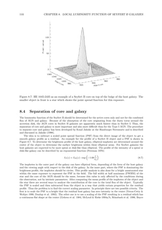
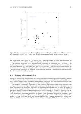
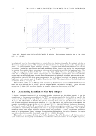
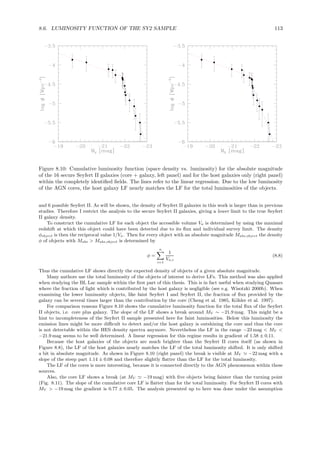

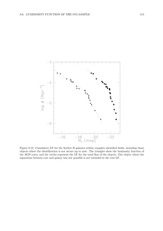
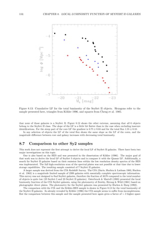

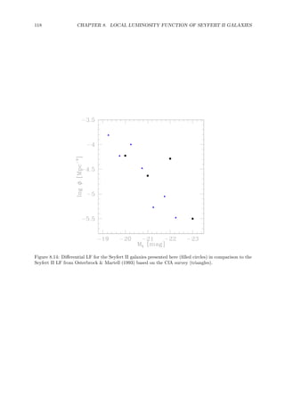
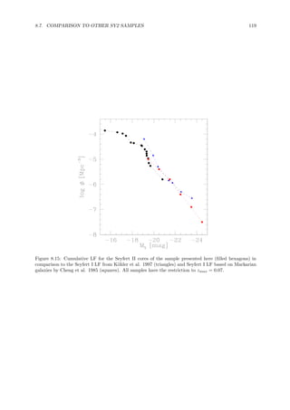
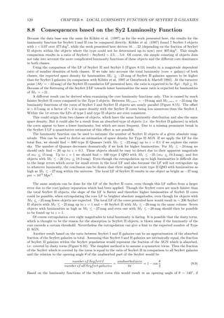
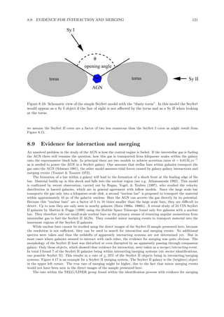
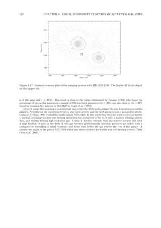
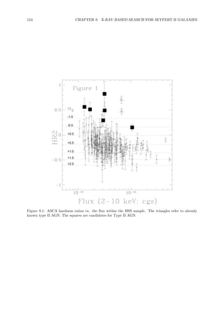
![9.3. FOLLOW UP SPECTROSCOPY OF HARDEST ASCA SOURCES 125
A1511+0758 / Object 9593 / B200 z=0.046
4000 5000 6000 7000 8000
wavelength [Å]
00.511.522.53
flux[10erg/cm²/sec/Å]−15
NeVOII]
NeIII
CaII−H
CaII−K
Hδ Hγ
He
HeHβ
OIII]
MgI NaI OI
[NII]
Hα
[NII]
[SII]
Figure 9.2: The CAFOS spectrum of the optical counter part of the ASCA source A1511+0758. Despite
a strong host galaxy, the Seyfert II core is clearly detectable.
energy band) and compared the position of the sources in the HR diagram with a grid of theoretical spectral
models. In Figure 9.1, for all sources, I plot the HR2 value versus the 2-10 keV flux and compare it with that
expected from a non-absorbed power-law model (fX ∝ E−αE
). This figure clearly shows a broadening and
flattening of the HR2 distribution going to fainter flux. The 2-10 keV “stacked” spectra of the sources with
fX ≤ 5 × 10⁻¹³
erg cm−2
sec−1
can be described by a power-law model with αE ∼ 0.4, thus it is clear that we are
beginning to detect those sources having a combined X-ray spectrum consistent with that of the 2-10 keV CXB.
It is worth noting the presence of many sources which seem to be characterized by a very flat 2-10 keV spectrum
with αE ≤ 0.5 and of a number of sources with “inverted” spectra (i.e. αE ≤ 0.0); this is particularly evident
below 5 × 10⁻¹³
erg cm−2
sec−1
where ∼ 50% of the sources seem to be described by αE ≤ 0.5 and ∼ 20% by
“inverted” spectra. These latter objects could represent a new population of very hard serendipitous sources or,
alternatively, a population of very absorbed sources as expected from the CXB synthesis models based on the
AGN Unification Scheme.
It is worth noting that the two objects marked as open triangles in Figure 9.1 have been spectroscopically
identified as Low Luminosity Type 2 AGN: one is the well known Seyfert 2 galaxy NGC 6552 (Fukazawa et al.
1994), while the other one is a nearby Seyfert 2 galaxy (UGC 12237) which was discovered in the HSS survey.
9.3 Follow up spectroscopy of hardest ASCA sources
Follow-up spectroscopy of hardest ASCA sources was done within two nights (10/11 March 2000) with the Calar
Alto1
2.2m telescope using the Calar Alto Faint Object Spectrograph (CAFOS). In total we tried to identify six
ASCA sources; pre-identification of bright objects using the objective prism plates of the Hamburg quasar Survey
(Hagen et al. 1995) reduced the number of candidates within the ASCA error circle (∼ 2 arcmin). Turning
the slit of the instrument allowed us to take spectra of at least two objects with one exposure. Exposure times
to identify the possible optical counterparts varied between 10 and 90 minutes. In total we observed 27 optical
sources, identifying 13 stars, three galaxies, one possible Seyfert 2 (A1313+3033) and one definite Seyfert 2 galaxy
(A1511+0758, see Fig. 9.2). For nine observed spectra it was not possible to give a clear identification. For the
clearly identified Seyfert 2 galaxy A1511+0758, we took a spectrum with higher resolution (∆λ ≃ 6 arcsec) on
the 14th of March using CAFOS again. We measured line properties within this spectrum, fitting Gaussian
profiles to the detected lines (Table 9.1). Using the direct images of A1511+0758, we performed a separation of
1German-Spanish Astronomical Center, Calar Alto, operated by the Max-Planck-Institut f¨ur Astronomie, Heidelberg,
jointly with the Spanish National Commission for Astronomy](https://image.slidesharecdn.com/6fabd339-d5aa-41a1-a40d-3283bf94795f-160804141441/85/doctor-125-320.jpg)
![126 CHAPTER 9. X-RAY BASED SEARCH FOR SEYFERT II GALAXIES
Table 9.1: Line properties in the spectrum of A1511+075
Hβ OIII OIII OI NII Hα NII
4861 ˚A 4959 ˚A 5007 ˚A 6300 ˚A 6548 ˚A 6562 ˚A 6583 ˚A
fluxa
0.4 3.2 6.3 0.3 1.3 11.0 4.5
EW [˚A] ∼ 0.7 6 12 ∼ 0.5 ∼ 2 ∼ 20 8
FWHM [˚A] ∼ 7 ∼ 9 8.3 ∼ 4 ∼ 9 ∼ 11 8.9
FWHM [km sec−1
] 430 540 500 200 410 500 410
a
Line flux in units 10−15
erg cm−2
sec−1
the core from the galaxy. Fitting a point spread function to the core we find the difference in magnitudes to be
mcore − mgalaxy = 1.43 in the Johnson-I band, and mcore − mgalaxy = 1.18 in the Johnson-R band. Since the
flux of the galaxy seems not to differ between the R and the I band, the core is significant brighter in the bluer
R-band, as expected for an AGN.
This investigations shows that it is possible to find Type II AGN. Never the less this does not solve the
question about the possible existence of Type II quasars. But the method described here to find possible Type II
AGN seems to be very promising as it detected one Type II AGN out of six candidates.](https://image.slidesharecdn.com/6fabd339-d5aa-41a1-a40d-3283bf94795f-160804141441/85/doctor-126-320.jpg)
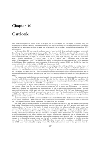
![128 CHAPTER 10. OUTLOOK
QSO.
To solve the question about the connection between Seyfert II and Seyfert I galaxies it is necessary to study
the Type II AGN at higher redshifts. One approach for this can be the optical identification of hard X-ray sources.
The XMM-Newton and Chandra X-ray mission will provide a lot of faint X-ray sources, where the hardest one
could be used to find Type II AGN and, if they exist, Type II QSO. Another way to achieve Seyfert II galaxies
at higher redshifts is the use of the objective prism plates of both, the HQS and HES. Here the search for objects
with [OII]3727 ˚A line can push the detection limit in redshift up to z ∼ 0.45. Using the MgII line at 2798 ˚A could
increase this limit to z ∼ 0.9.](https://image.slidesharecdn.com/6fabd339-d5aa-41a1-a40d-3283bf94795f-160804141441/85/doctor-128-320.jpg)
![Chapter 11
Appendix
All positions throughout this thesis are given in J2000.0
11.1 Tables to the HRX-BL Lac sample
Table 11.1: Objects from the NVSS/BSC correlation
α δ Name Redshift Classification
07 01 32.1 25 09 51 1RXS J070132.1+250950
07 04 27.0 63 18 56 KUG 0659+633 0.095 G
07 07 02.9 27 06 51 1RXS J070702.9+270650
07 07 13.5 64 35 58 VII Zw 118 0.080 Sy1
07 09 07.6 48 36 57 NGC 2329 0.019 G S0-:
07 10 24.2 22 40 13 MG2 J071027+2239
07 10 30.0 59 08 08 87GB 070609.2+591323 0.125 BL Lac
07 11 48.0 32 19 02 PGC 020369 0.067 G
07 13 39.7 38 20 43 IRAS F07102+3825 0.123 NLSy1
07 18 00.7 44 05 27 IRAS F07144+4410 0.061 Sy1
07 20 19.1 23 49 04 1RXS J072019.1+234904
07 21 32.9 26 09 39 1RXS J072132.9+260939
07 21 53.2 71 20 31 0716+714 BL Lac
07 22 17.4 30 30 52 HS 0719+3036 0.100 Sy1.5
07 29 27.4 24 36 25 2MASX1 J0729277+24362 G
07 31 52.4 28 04 23 2MASX1 J0731526+28043
07 32 21.5 31 37 51 1RXS J073221.5+313750 0.170 G
07 36 24.8 39 26 08 FBS 0732+396 0.118 Sy1
07 40 58.5 55 25 33 CGCG 262-019 0.034 GGroup
07 41 44.8 74 14 45 ZwCl 0735.7+7421 0.216 GClstr
07 42 32.9 49 48 30 UGC 03973 0.022 Sy1.2
07 42 50.3 61 09 31 87GB 073825.7+611711 star (K0)
07 43 18.7 28 53 07 Sigma Gem star (K1IIIRSCVn)
07 44 05.6 74 33 56 MS 0737.9+7441 0.315 BL Lac
07 45 41.2 31 42 50 [HB89] 0742+318 0.461 Sy1
07 47 29.4 60 56 01 UGC 04013 0.029 Sy1.2
07 49 06.2 45 10 40 B3 0745+453 0.190 Sy1
07 49 29.4 74 51 43 87GB[BWE91] 0743+7458 0.607 BL Lac
07 51 22.1 55 11 57 1RXS J075122.1+551156 0.340 Sy1
07 52 43.6 45 56 53 NPM1G +46.0092 0.060 G
08 01 32.3 47 36 19 87GB 075755.8+474440 0.158 Sy1
(continued on the next page)
X-ray count rate limit hcps ≥ 0.09 (RASS-BSC), radio flux limit fR(1.4 GHz) ≥ 2.5 mJy (NVSS)
129](https://image.slidesharecdn.com/6fabd339-d5aa-41a1-a40d-3283bf94795f-160804141441/85/doctor-129-320.jpg)
![130 CHAPTER 11. APPENDIX
The objects of the NVSS/BSC correlation
α δ Name Redshift Classification
08 01 47.8 56 33 16 NGC 2488 0.029 G, S0-:
08 05 25.8 75 34 24 WN B0759.1+7542 0.121 BL Lac
08 06 25.5 59 31 06 87GB 080212.8+593933 BL Lac
08 09 38.5 34 55 45 MG2 J080937+3455 0.082 BL Lac
08 09 49.2 52 18 56 87GB 080601.8+522753 0.138 BL Lac
08 10 59.0 76 02 45 PG 0804+761 0.100 Sy1
08 15 17.8 46 04 29 KUG 0811+462 0.041 Sy1.5
08 19 26.6 63 37 41 KOS NP6 038 0.118 G, E
08 19 29.5 70 42 21 1RXS J081929.5+704221 0.001 HolmbergII
08 22 09.5 47 06 01 RGB J0822+470 0.127 GClstr (Abell 0646)
08 32 25.1 37 07 37 FIRST J083225.3+37073 0.091 Sy1.2
08 32 51.9 33 00 11 RX J0832.8+3300 0.671 BL Lac
08 36 58.3 44 26 13 [HB89] 0833+446 0.255 QSO
08 38 11.0 24 53 36 NGC 2622 0.029 Sy1.8
08 41 25.1 70 53 43 [HB89] 0836+710 2.172 Blazar
08 42 03.4 40 18 30 KUV 08388+4029 0.152 Sy1
08 42 55.9 29 27 52 ZwCl 0839.9+2937 0.194 GClstr
08 59 16.5 83 44 50 1RXS J085916.5+834450 0.327 BL Lac
08 59 30.1 74 55 10 RX J0859.5+7455 0.276 Sy1
09 09 53.9 31 05 58 MG2 J090953+3104 0.274 BL Lac
09 13 24.6 81 33 18 1RXS J091324.6+813318 0.639 BL Lac
09 15 52.2 29 33 35 B2 0912+29 / TON 0396 BL Lac
09 16 51.8 52 38 29 87GB 091315.6+525108 0.190 BL Lac
09 20 15.3 86 02 54 1RXS J092015.3+860254
09 23 43.0 22 54 37 CGCG 121-075 0.032 Sy1
09 25 12.3 52 17 17 MRK 0110 0.035 Sy1
09 27 02.8 39 02 21 [HB89] 0923+392 0.695 Sy1
09 28 04.2 74 47 15 87GB 092308.0+745942 0.638 BL Lac
09 30 37.1 49 50 28 1ES 0927+500 0.186 BL Lac
09 33 46.5 62 49 44 1RXS J093346.5+624943 star
09 35 27.4 26 17 14 RX J0935.4+2617 0.122 Sy1
09 47 13.2 76 23 17 RBS 0797 0.354 LINER
09 52 25.8 75 02 17 RX J0952.4+7502 0.178 BL Lac
09 55 34.7 69 03 38 MESSIER 081 -0.00011 LINER/Sy1.8
09 55 50.4 69 40 52 MESSIER 082 0.00068 Starburst G
09 59 29.8 21 23 40 87GB 095643.1+213755 0.367 BL Lac
10 00 28.9 44 09 10 RX J1000.4+4409 0.154 GClstr
10 02 35.9 32 42 19 NGC 3099 0.051 G
10 05 42.2 43 32 44 IRAS 10026+4347 0.178 Sy1
10 06 39.1 25 54 51 PGC 029375 0.116 GClstr
10 08 11.5 47 05 26 RX J1008.1+4705 0.343 BL Lac
10 09 16.7 71 10 40 87GB 100504.8+712548 0.193 GClstr
10 10 27.9 41 32 42 [HB89] 1007+417 0.612 QSO
10 12 44.4 42 29 59 B3 1009+427 0.376 BL Lac
10 15 04.3 49 26 04 [HB89] 1011+496 0.200 BL Lac
10 16 16.4 41 08 18 FIRST J101616.8+41081 0.281 BL Lac
10 16 55.5 73 23 59 NGC 3147 0.009 Sy2
10 17 18.0 29 14 39 IRAS F10144+2929 0.048 Sy1
10 19 00.8 37 52 50 FIRST J101900.4+37524 0.133 Sy1
10 19 12.1 63 58 03 MRK 141 0.042 Sy1.5
(continued on the next page)
X-ray count rate limit hcps ≥ 0.09 (RASS-BSC), radio flux limit fR(1.4 GHz) ≥ 2.5 mJy (NVSS)](https://image.slidesharecdn.com/6fabd339-d5aa-41a1-a40d-3283bf94795f-160804141441/85/doctor-130-320.jpg)
![11.1. TABLES TO THE HRX-BL LAC SAMPLE 131
The objects of the NVSS/BSC correlation
α δ Name Redshift Classification
10 22 12.5 51 24 06 MS 1019.0+5139 0.141 BL Lac
10 22 28.9 50 06 30 ABELL 0980:[CAE99] 0.158 G
10 30 58.8 31 03 06 [HB89] 1028+313 0.178 Sy1
10 31 05.7 82 33 27 1RXS J103105.7+823327 star F2V
10 31 18.6 50 53 41 1ES 1028+511 0.361 BL Lac
10 32 14.3 40 16 07 [BBN91] 102920+403136 0.078 GClstr
10 34 23.1 73 45 25 NGC 3252 0.004 G, SBd?sp
10 34 38.7 39 38 34 KUG 1031+398 0.042 Sy1
10 34 59.5 30 41 39 Abel 1045 0.137 GClstr
10 38 46.7 53 30 02 SN 1991N 0.003 SNR in NGC3310
10 40 43.7 39 57 06 IRAS F10378+4012 0.139 Sy2
10 44 27.6 27 18 13 1RXS J104427.6+271813 G
10 44 39.4 38 45 42 CGCG 212-045 0.036 G
10 45 20.5 45 34 04 1RXS J104520.5+453404 star B8V
10 51 25.1 39 43 30 FIRST J105125.3+39432 0.498 BL Lac
10 55 44.0 60 28 10 1RXS J105544.0+602810 star
10 57 23.5 23 03 17 1RXS J105723.5+230317 0.378 BL Lac
10 58 25.9 56 47 16 RX J1058+5647 prob. GClstr
10 58 37.5 56 28 16 87GB 105536.5+564424 0.144 BL Lac
11 00 21.3 40 19 33 FIRST J110021.0+40192 0.225 BL Lac
11 04 12.4 76 58 59 PG 1100+772 0.312 QSO (Opt.var.)
11 04 27.1 38 12 32 MRK 421 0.030 BL Lac
11 06 43.5 72 34 07 NGC 3516 0.009 Sy1.5
11 11 31.2 34 52 12 FIRST J111130.8+34520 0.212 BL Lac
11 11 37.2 40 50 31 ABELL 1190:[SBM98] 0.079 GClstr
11 14 22.6 58 23 18 8C 1111+586 0.206 GClstr
11 17 06.3 20 14 10 87GB 111429.0+203022 0.137 BL Lac
11 18 03.6 45 06 57 LEDA 139560 0.106 Sy1
11 19 08.1 21 19 15 PG 1116+215 0.176 Sy1
11 20 47.5 42 12 17 1ES 1118+424 0.124 BL Lac
11 21 09.9 53 51 25 RX J1121.1+5351 0.103 Sy1
11 23 49.2 72 30 02 RX J1123+7230 BL Lac
11 23 57.4 21 29 14 [CWH99] 112356.7+2129 0.199 GClstr
11 31 08.9 31 14 09 TON 0580 0.289 QSO
11 31 21.4 33 34 47 RX J1131.3+3334 0.222 G
11 32 22.4 55 58 28 RX J1132.3+5558 0.051 GClstr
11 36 26.6 70 09 32 MRK 180 0.046 BL Lac
11 36 29.4 21 35 53 MRK 739b 0.030 Sy1
11 36 30.9 67 37 08 HS 1133+6753 0.135 BL Lac
11 41 16.2 21 56 25 PG 1138+222 0.063 Sy1
11 44 29.9 36 53 14 KUG 1141+371 0.040 Sy1
11 45 09.3 30 47 25 [HB89] 1142+310 0.060 Sy1.5
11 47 54.9 22 05 48 RX J1147.9+2205 0.276 BL Lac
11 49 30.4 24 39 28 RGB J1149+246 0.402 BL Lac
11 53 24.4 49 31 09 [HB89] 1150+497 0.334 QSO
11 55 18.9 23 24 32 MCG +04-28-097 0.143 G
11 57 56.1 55 27 17 NGC 3998 0.003 Sy1;LINER
12 03 08.9 44 31 55 NGC 4051 0.002 Sy1.5
12 03 43.3 28 36 02 RX J1203.7+2836 0.373 Sy1
12 05 11.7 39 20 43 RX J1205.1+3920 0.037 GClstr
(continued on the next page)
X-ray count rate limit hcps ≥ 0.09 (RASS-BSC), radio flux limit fR(1.4 GHz) ≥ 2.5 mJy (NVSS)](https://image.slidesharecdn.com/6fabd339-d5aa-41a1-a40d-3283bf94795f-160804141441/85/doctor-131-320.jpg)
![132 CHAPTER 11. APPENDIX
The objects of the NVSS/BSC correlation
α δ Name Redshift Classification
12 09 46.0 32 17 03 FIRST J120945.2+32170 0.145 Sy1
12 11 58.1 22 42 36 RX J1211.9+2242 0.455 BL Lac
12 13 45.2 36 37 55 NGC 4190 0.001 G
12 15 06.7 33 11 30 NGC 4203 0.004 LINER
12 17 52.1 30 07 05 ON 325 / B2 1215+30 0.130 BL Lac
12 18 27.0 29 48 53 NGC 4253 0.013 Sy1.5
12 20 44.5 69 05 33 RX J1220+6905
12 21 21.7 30 10 41 FBQS J1221+3010 0.182 BL Lac
12 21 44.4 75 18 48 MRK 205 0.071 Sy1
12 24 54.9 21 22 52 PG 1222+216 0.435 Blazar
12 25 12.5 32 13 54 MAPS-NGP O-267-076115 0.059 GClstr
12 26 23.9 32 44 31 NGC 4395:[R97] 12 0.242 Sy1
12 30 14.2 25 18 05 MG2 J123013+2517 0.135 BL Lac
12 31 32.5 64 14 20 [HB89] 1229+645 0.164 BL Lac
12 32 03.6 20 09 30 MRK 771 0.063 Sy1
12 36 51.1 45 39 07 CGCG 244-033 0.030 Sy1.5
12 36 58.8 63 11 11 ABELL 1576:[HHP90] 0.302 G
12 37 05.6 30 20 03 FIRST J123705.5+30200 0.700 BL Lac
12 37 39.2 62 58 43 [HB89] 1235+632 0.297 BL Lac
12 38 08.3 53 26 04 87GB 123550.3+534219 0.347 Sy1
12 39 23.1 41 32 45 FIRST J123922.7+41325 BL Lac
12 41 41.2 34 40 32 FIRST J124141.3+34403 BL Lac
12 41 44.4 35 03 53 NGC 4619 0.023 Sy1
12 42 11.3 33 17 03 WAS 61 0.044 Sy1
12 43 12.5 36 27 43 TON 0116 BL Lac
12 47 01.3 44 23 25 RGB J1247+443 AGN
12 48 18.9 58 20 31 PG 1246+586 BL Lac
12 50 52.5 41 07 13 MESSIER 94 0.001 LINER
12 53 01.0 38 26 29 FIRST J125300.9+38262 0.360 BL Lac
12 57 31.7 24 12 46 1ES 1255+244 0.141 BL Lac
13 02 55.6 50 56 21 RX J1302.9+5056 0.688 BL Lac
13 05 52.6 30 54 06 ABELL 1677 0.183 GClstr
13 13 27.2 36 35 42 NGC 5033 0.003 Sy1.9
13 19 57.2 52 35 33 RX J1319.9+5235 0.092 Sy
13 20 16.3 33 08 29 RX J1320.1+3308 0.036 GClstr
13 22 48.5 54 55 27 RX J1322.8+5455 0.064 Sy1
13 24 00.2 57 39 19 87GB 132204.6+575429 0.115 BL Lac
13 25 49.2 59 19 37 ABELL 1744:[HHP90] 0.151 GClstr
13 26 15.0 29 33 33 87GB 132354.7+294853 0.431 BL Lac
13 34 47.5 37 11 00 BH CVn star (F2IVRSCVn)
13 35 08.2 20 46 41 RX J1335.1+2046 star
13 37 18.8 24 23 07 [HB89] 1334+246 0.108 Sy1
13 40 29.9 44 10 08 87GB 133822.3+442514 0.548 BL Lac
13 41 04.8 39 59 42 B3 1338+402 0.163 BL Lac
13 41 52.6 26 22 30 1RXS J134152.6+262230 GClstr
13 45 45.1 53 33 01 87GB 134352.4+534755 0.135 Sy1
13 48 52.6 26 35 41 ABELL 1795:[MK91] 0.062 GClstr
13 53 04.8 69 18 33 UGC 08823 0.029 Sy1.5
13 53 28.2 56 01 02 RX J1353.4+5601 0.370 BL Lac
13 54 20.2 32 55 47 UGC 08829 0.026 Sy1
(continued on the next page)
X-ray count rate limit hcps ≥ 0.09 (RASS-BSC), radio flux limit fR(1.4 GHz) ≥ 2.5 mJy (NVSS)](https://image.slidesharecdn.com/6fabd339-d5aa-41a1-a40d-3283bf94795f-160804141441/85/doctor-132-320.jpg)
![11.1. TABLES TO THE HRX-BL LAC SAMPLE 133
The objects of the NVSS/BSC correlation
α δ Name Redshift Classification
13 55 15.9 56 12 44 RX J1355.2+5612 0.122 Sy1
13 55 53.3 38 34 28 MRK 464 0.051 Sy1.5
14 04 50.2 65 54 34 RX J1404.8+6554 0.364 BL Lac
14 06 22.2 22 23 50 PG 1404+226 0.098 Sy
14 10 31.6 61 00 21 RX J1410.5+6100 0.384 BL Lac
14 13 42.6 43 39 38 MAPS-NGP O-221-004710 0.089 G
14 13 58.3 76 44 56 1RXS J141358.3+764456 0.068 Sy2
14 17 56.8 25 43 29 1E 1415+259 0.237 BL Lac
14 17 59.6 25 08 18 SN 1984Z 0.017 SNR in NGC5548
14 21 36.4 49 33 05 MCG +08-26-021 0.072 GClstr
14 21 39.7 37 17 43 RX J1421.6+3717 0.160 GClstr
14 22 39.1 58 02 00 RGB J1422+580 0.638 BL Lac
14 23 13.4 50 55 37 87GB 142127.2+510856 0.274 Sy1
14 23 53.6 40 15 33 RX J1423.8+4015 0.082 GClstr
14 23 56.0 26 26 30 1RXS J142356.0+262630 Prob. GClstr
14 26 01.3 37 49 36 ABELL 1914 0.171 GClstr
14 27 00.5 23 48 03 PG 1424+240 BL Lac
14 28 32.6 42 40 28 1ES 1426+428 0.129 BL Lac
14 31 04.8 28 17 16 MRK 684 0.046 Sy1
14 31 06.2 25 38 15 RX J1431.1+2538 0.096 GClstr
14 32 36.0 31 38 55 RX J1432.5+3138 0.132 GClstr
14 39 17.7 39 32 49 PG 1437+398 BL Lac
14 42 07.7 35 26 32 MRK 478 0.079 Sy1
14 42 18.9 22 18 20 UGC 09480 0.097 GClstr
14 43 02.8 52 01 41 3C 303 0.141 G
14 44 33.9 63 36 04 MS 1443.5+6349 0.299 BL Lac
14 48 01.0 36 08 33 [WB92] 1446+3620 BL Lac
14 49 32.3 27 46 30 RBS 1434 0.228 BL Lac
14 51 08.5 27 09 33 PG 1448+273 0.065 Sy1
14 56 03.4 50 48 24 RX J1456+5048 0.480 BL Lac
14 57 15.4 22 20 26 MS 1455.0+2232 0.258 GClstr
14 58 27.3 48 32 50 RX J1458.4+4832 0.539 BL Lac
15 00 20.7 21 22 14 LEDA 140447 0.153 G
15 01 01.7 22 38 12 MS 1458.8+2249 0.235 BL Lac
15 04 13.1 68 56 10 [HB89] 1503+691 0.318 Sy1
15 07 44.6 51 27 10 MRK 845 0.046 Sy1
15 08 42.2 27 09 11 RBS 1467 0.270 BL Lac
15 10 40.8 33 35 15 RX J1510.6+3335 0.116 BL Lac
15 14 43.1 36 50 59 [HB89] 1512+370 0.371 QSO/Sy1?
15 17 47.3 65 25 23 1517+656 0.702 BL Lac
15 21 53.0 20 58 30 1RXS J152153.0+205830 star M9
15 23 46.0 63 39 30 4C +63.22 0.204 G
15 29 07.5 56 16 05 IRAS F15279+5626 0.099 Sy1
15 32 02.3 30 16 32 87GB 152959.0+302636 0.064 BL Lac
15 32 53.7 30 21 03 RBS 1509 0.361 LINER/GClstr
15 33 24.9 34 16 41 87GB 153121.5+342710 BL Lac
15 35 01.1 53 20 42 1ES 1533+535 0.890 BL Lac
15 35 52.0 57 54 04 MRK 290 0.030 Sy1
15 39 50.3 30 43 05 RX J1539.8+3043 0.097 GClstr
15 40 16.4 81 55 05 1ES 1544+820 BL Lac
(continued on the next page)
X-ray count rate limit hcps ≥ 0.09 (RASS-BSC), radio flux limit fR(1.4 GHz) ≥ 2.5 mJy (NVSS)](https://image.slidesharecdn.com/6fabd339-d5aa-41a1-a40d-3283bf94795f-160804141441/85/doctor-133-320.jpg)
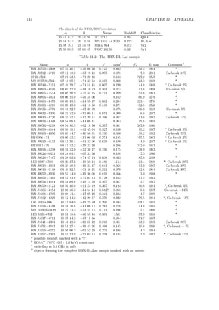
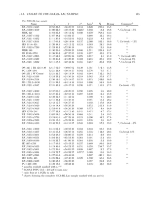
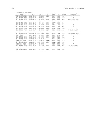
![11.1. TABLES TO THE HRX-BL LAC SAMPLE 137
Table 11.3: Photometry of HRX-BL Lac
Name Jul. Date Exp. Timea
B [mag] 1σ[ mag] Standardb
RX J0859+8345 2451669.3484 600 19.73 0.19 P066-B
RX J0909+3105 2451667.3408 240 18.28 0.07 P313-D
RX J0913+8133 2451667.3582 600 20.7 0.10 P125-E P006-D
RX J0916+5238 2451667.3471 600 18.33 0.05 P313-D P125-E
RX J0924+0533 2451669.3724 500 19.60 0.09 P547-B
RX J0928+7447 2451667.3694 800 20.7 0.10 P006-D P018-E
RX J0952+7502 2451669.3713 500 19.20 0.19 P066-B P018-B
RX J0959+2133 2451669.3817 400 19.06 0.06 P547-B P371-A
RX J1008+4705 2451669.3959 400 19.92 0.10 P212-D P167-C
RX J1012+4229 2451669.3890 300 18.42 0.05 P371-A P212-D
RX J1016+4108 2451669.4036 200 19.46 0.05 P167-C P212-D
RX J1051+3943 2451665.3856 800 19.0 0.18 P213-A P551-C
RX J1054+3855 2451663.3643 120 17.8 P213-A
RX J1054+3855 2451665.3759 300 17.3 P213-A
RX J1056+0252 2451667.3871 900 19.39 0.05 P018-E P551-C
RX J1057+2303 2451663.3798 600 19.74 0.05 P213-A P373-D
RX J1100+4019 2451667.4236 300 18.56 0.05 P214-E P214-D
RX J1107+1502 2451667.4153 400 18.4 0.20 P491-A
RX J1111+3452 2451667.4031 800 19.7 0.05 P551-C P491-A
RX J1120+4212 2451667.4313 200 18.0 0.20 P214-D
RX J1149+2439 2451667.4403 400 19.0 0.20 P265-C
RX J1153+3617 2451663.3941 120 17.51 P273-D P265-C
RX J1211+2242 2451663.4011 500 19.55 0.05 P265-C P376-F
RX J1230+2518 2451663.4146 60 16.04 0.10 P376-F P377-A
RX J1230+2518 2451667.4591 150 15.94 0.05 P377-A
RX J1231+6414 2451667.4515 300 18.0 0.20 P064-A
RX J1237+6258 2451663.4359 600 18.85 0.05 P095-D
RX J1239+4132 2451663.4240 600 20.34 0.10 P377-A
RX J1241+3440 2451663.4466 600 20.18 0.16 P267-C
RX J1243+3627 2451667.4660 300 16.60 0.10 P377-A P267-E
RX J1248+5820 2451667.4749 200 14.89 0.05 P267-E
RX J1253+3826 2451663.4631 500 18.9 0.20 P267-C
RX J1302+5056 2451663.4761 600 19.3 0.20 P131-A
RX J1324+5739 2451667.4944 200 17.75 0.05 P219-D P096-A
RX J1326+2913 2451663.4868 500 18.69 0.05 P131-A P173-F
RX J1340+4410 2451663.4965 400 19.25 0.11 P173-F
RX J1341+3959 2451667.4868 400 18.6 0.22 P219-D
RX J1353+5600 2451667.5000 600 19.10 0.05 P096-A P097-A
RX J1404+6554 2451663.5053 600 19.36 0.08 P066-A
RX J1410+6100 2451667.5774 1200 19.89 0.07 P066-E
RX J1422+5801 2451663.5169 400 17.82 0.07 P098-A
RX J1444+6336 2451663.5600 600 19.7 0.20 P067-E
RX J1449+2746 2451667.5362 600 20.03 0.10 P382-B PKS1510-089
RX J1456+5048 2451663.5506 400 18.57 0.07 P067-E
RX J1458+4832 2451667.5146 1200 20.37 0.09 P382-B
RX J1501+2238 2451667.6018 180 15.53 0.05 P066-E P382-B
RX J1508+2709 2451663.5842 600 18.77 0.05 1517+656 P327-G
RX J1510+3335 2451663.6097 500 18.50 0.07 P385-B P327-G
RX J1517+6525 2451663.5756 150 16.87 0.04 Standard field
RX J1535+5320 2451663.6192 400 18.9 0.20 P327-G P008-B
a
exposure time in seconds
b
photometric standard from the GSPC used for calibration](https://image.slidesharecdn.com/6fabd339-d5aa-41a1-a40d-3283bf94795f-160804141441/85/doctor-137-320.jpg)
![138 CHAPTER 11. APPENDIX
Photometry of HRX-BL Lac
Name Jul. Date Exp. Time B [mag] 1σ[ mag] Standard
RX J1544+8155 2451663.6287 300 17.1 0.18 P008-B
RX J1554+2011 2451663.6021 300 18.45 0.05 P327-G P385-B
RX J1554+2414 2451663.6413 300 20.4 0.20 P385-D](https://image.slidesharecdn.com/6fabd339-d5aa-41a1-a40d-3283bf94795f-160804141441/85/doctor-138-320.jpg)
![11.2. FORMULAE TO THE HRX-BL LAC DESCRIPTION 139
Table 11.4: BL Lac candidates which turned out to be no BL Lacs
Name α δ z Type
RX J0751+5512 07 51 22.3 +55 12 09 0.340 Sy1
RX J0754+4316 07 54 07.9 +43 16 10 0.388 Sy1
RX J0806+7248 08 06 38.9 +72 48 20 0.097 NLSy1
RX J0807+3400 08 07 30.8 +34 00 42 0.208 Gal. (Ca break 51%)
RX J0819+6337 08 19 25.8 +63 37 26 0.118 Gal. (Ca break 59%)
RX J0826+3108 08 26 53.5 +31 08 05 0.205 Gal. (Ca break 59%)
RX J0900+2054 09 00 35.5 +20 54 51 0.31 Gal. (Ca break 42%)
RX J0918+3156 09 18 33.9 +31 56 20 0.451 Sy1
RX J1005+4332 10 05 41.0 +43 32 27 0.178 Sy1
RX J1054+1506 10 54 43.0 +15 06 57 0.582 Sy1
RX J1119+4130 11 19 07.1 +41 30 15 0.094 Sy1a
RX J1131+3334 11 31 20.9 +33 34 46 0.222 Gal.b
RX J1226+3244 12 26 24.0 +32 44 33 0.242 Sy1
RX J1238+5325 12 38 08.2 +53 25 56 0.347 Sy1
RX J1324+2802 13 24 22.8 +28 02 32 0.124 Sy1
RX J1345+5332 13 45 45.6 +53 32 55 0.135 Sy1
RX J1353+2809 13 53 08.4 +28 09 09 0.516 Sy1
RX J1408+2409 14 08 27.3 +24 09 29 0.129 NLSy1
RX J1413+7644 14 13 58.0 +76 44 57 0.068 Sy2
RX J1424+2514 14 24 24.5 +25 14 28 0.237 Gal.c
RX J1434+2317 14 34 44.9 +23 17 43 0.100 Sy1
RX J1535+7948 15 35 31.7 +79 48 49 0.072 Sy1.5
RX J1551+1911 15 51 55.1 +19 11 08 2.821 QSO
RX J1701+3404 17 01 02.6 +34 04 09 0.094 Sy1
a)
two more galaxies (z = 0.096, z = 0.094) within the BSC error circle
b)
calcium break ∼ 46%. The core shows strong [NII], Hα and [SII] lines - Seyfert II core?
c)
equivalent width of Hα = 67 ˚A
11.2 Formulae to the HRX-BL Lac description
11.2.1 Parabola
Given three points [xi, yi]; i = [1..3] the parameters for a parabola y = a · x2
+ b · x + c are given by
a =
y3 − y1 − y2−y1
x2−x1
· x3 + x1 · y2−y1
x2−x1
((x2
3 + x2
1 · x3
x2−x1
− x2
2 · x3
x2−x1
− x2
1) − x3
1) · (x2 − x1)
+
x1 · x2
2
x2 − x1
(11.1)
b =
y2 − y1 + a · x2
1 − a · x2
2
x2 − x1
(11.2)
c = y1 − a · x2
1 − b · x1 (11.3)
The peak of the parabola occurs at the point xpeak which is simply
xpeak =
−b
2a
(11.4)
with a peak value
ypeak =
a · b2
4
−
b2
2a
+ c (11.5)
11.2.2 Student’s distribution
To test the probability of a correlation between n observed pairs of parameter [Xi, Yi]i=1..n the hypothesis H0 is
tested, if the two parameters are not correlated. The Pearsons correlation-coefficient rXY can be used for this](https://image.slidesharecdn.com/6fabd339-d5aa-41a1-a40d-3283bf94795f-160804141441/85/doctor-139-320.jpg)
![140 CHAPTER 11. APPENDIX
Table 11.5: Seyfert II sample
Name α δ ESO-field z Cand.a
Typeb
HE 0058-4740 01 01 14.2 -47 24 31 195 0.025 2 2
HE 0113-5027 01 15 55.3 -50 11 22 195 0.024 1 1
HE 0047-5107 00 49 45.2 -50 50 41 195 0.060 1 2
HE 0209-4956 02 10 52.5 -49 41 56 197 0.047 1 1
HE 0348-5027 03 50 23.0 -50 18 10 201 0.037 1 1
HE 0506-5047 05 08 06.3 -50 43 52 203 0.049 1 1
HE 0508-5016 05 10 14.4 -50 12 48 203 0.049 2 1
HE 0411-4131 04 13 24.0 -41 23 44 303 0.027 2 1
HE 0201-3029 02 03 25.1 -30 14 55 414 0.036 1 1
HE 0235-2913 02 37 15.2 -29 00 22 416 0.050 2 3
HE 0246-3122 02 49 03.9 -31 10 21 416 0.020 1 1
HE 0254-3223 02 56 21.5 -32 11 09 417 0.016 1 1
HE 0436-3017 04 29 52.4 -30 15 22 421 0.055 2 1
HE 0436-2908 04 38 48.3 -29 02 18 421 0.044 2 1
HE 1132-3015 11 35 25.7 -30 32 26 439 0.031 1 3
HE 1202-2937 12 04 51.0 -29 54 04 440 0.059 2 3
HE 1146-3206 11 49 31.0 -32 23 04 440 0.021 1 1
HE 0051-2420 00 53 54.4 -24 04 36 474 0.056 1 1
HE 0128-2609 01 30 26.0 -25 53 47 476 0.031 1 3
HE 1045-2453 10 48 23.5 -25 09 43 501 0.012 1 1
HE 1103-2519 11 05 54.7 -25 35 20 502 0.012 2 3
HE 1223-2319 12 26 02.4 -23 36 22 506 0.048 1 1
HE 1252-2640 12 54 56.3 -26 57 02 507 0.058 1 1
HE 1331-2311 13 34 39.6 -23 26 48 509 0.034 1 1
HE 1335-2344 13 37 49.9 -23 59 41 509 0.030 1 1
HE 0136-2042 01 39 20.4 -20 27 12 543 0.045 1 1
HE 0154-2047 01 57 00.7 -20 33 02 543 0.045 2 3
HE 0448-2125 04 50 20.3 -21 20 20 552 0.032 2 3
HE 1020-1925 10 22 57.1 -19 40 47 568 0.022 2 2
a)
candidate type within selection process: 1 = secure, 2 = probably
b)
spectroscopic type: 1 = Seyfert II, 2 = probable SyII, 3 = Sy2, LINER, or NELG
test. This coefficient has a value within the interval [−1; +1]. If rXY = 0, no correlation is detected. Assuming
that X and Y are normal distributed then rXY can be used to test if X and Y are independent. If the (unknown)
correlation coefficient ρ = 0 then
t =
rXY ·
√
n − 2
√
1 − rXY
2
(11.6)
is the realization of a t-distributed random variable with n − 2 degrees of freedom. The t-distribution, also called
Student’s distribution, is tabulated for different n and t values (e.g. Bronstein & Semendjajew 1987). This results
in a significance level on which the assumption that X and Y are uncorrelated can be rejected.
11.3 Tables to the Seyfert II sample
Table 11.6: False Seyfert II candidates
Name α δ ESO field z type
HE 0146-5217 01 48 00.0 -52 02 59 197 0.047 galaxy
HE 0346-4856 03 47 46.6 -48 47 17 201 0.050 galaxy
HE 0345-5023 03 46 43.7 -50 13 53 201 0.054 galaxy
(continued on the next page)](https://image.slidesharecdn.com/6fabd339-d5aa-41a1-a40d-3283bf94795f-160804141441/85/doctor-140-320.jpg)
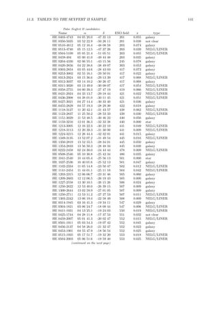
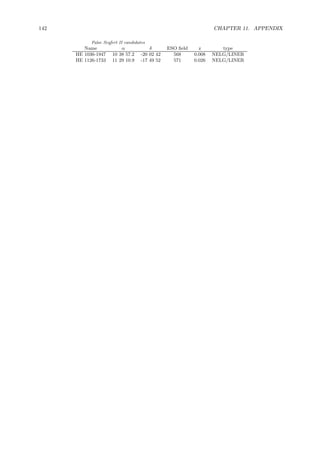


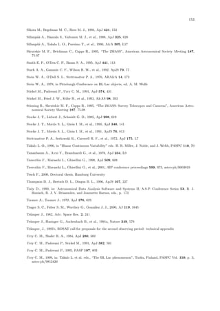
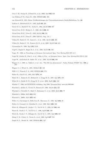


![ALMA Detection of [OIII] 88μmatz=12.33:Exploring the Nature and Evolution of ...](https://cdn.slidesharecdn.com/ss_thumbnails/zavala2024apjl977l9-250125143557-29e4ae2d-thumbnail.jpg?width=640&height=640&fit=bounds)


