This dissertation by Sameer Patel examines multi-wavelength analysis of active galactic nuclei (AGNs) and their significance in understanding the universe. It discusses current research methods and the various types of AGNs, which are powerful emitters of electromagnetic radiation yet harbor many unexplained phenomena. The work also touches upon the unification model of AGNs, aiming to provide a comprehensive overview of their classification and behaviors across different wavelengths.

1. Multi-Wavelength Analysis of Active
Galactic Nuclei
A dissertation submitted as partial ful

2. lment
of the
100-hour certi

3. cate course
in
Astronomy & Astrophysics
by
Sameer Patel
M.P. Birla Institute of Fundamental Research
Bangalore, India
December 2014

4. Declaration
I, Sameer Patel, student of M.P. Birla Institute of Fundamental Research, Bangalore,
hereby declare that the matter embodied in this dissertation has been compiled and
prepared by me on the basis of available literature on the topic titled,
Multi-Wavelength Analysis of Active Galactic Nuclei
as a partial ful

5. llment of the 100 Hour Certi

6. cate Course in Astronomy and Astro-physics,
2014. This dissertation has not been submitted either partially or fully to any
university or institute for the award of any degree, diploma or fellowship.
Date:
Place:
Signature
Director,
M.P. Birla Institute of Fundamental Research,
Bangalore
i

7. M.P. Birla Institute of Fundamental Research
Bangalore, India
Abstract
Multi-Wavelength Analysis of Active Galactic Nuclei
by Sameer Patel
This dissertation explores the current research methods and analysis adopted for the
study of Active Galactic Nuclei in all wavelengths of the electromagnetic radiation.
Being the most violent objects that one can see in the present Universe, AGNs have been
attributed to emitting radiation in all wavelengths and still exhibit various unexplained
phenomena, alongside with being the probes to the very early Universe. The uni

8. cation
of the AGN model is also included for completeness, albeit not con

9. rmed in its entirety.

10. Acknowledgements
I would never have been able to

11. nish my dissertation without help from friends, and
support from the team at MPBIFR, Bangalore.
I would also like to thank Dr. Babu for constantly reminding us to complete the dis-sertation
timely, and Ms. Komala for guiding me to coast through countless papers
online for reference. I would like to thank Rishi Dua, who as a good friend, was always
willing to help me and give his best suggestions, and Aakash Masand, who helped me
correct typographical errors and grammatical mistakes after painfully proofreading the

12. nal draft.
I would also like to thank my parents. They were always supporting me and encouraging
me with their best wishes.
iii

13. Contents
Declaration i
Abstract ii
Acknowledgements iii
List of Figures vii
List of Tables ix
Abbreviations x
1 Introduction 1
1.1 The History of AGNs . . . . . . . . . . . . . . . . . . . . . . . . . . . . . . 1
1.2 Active Galactic Nuclei . . . . . . . . . . . . . . . . . . . . . . . . . . . . . 1
1.3 The Taxonomy of AGNs . . . . . . . . . . . . . . . . . . . . . . . . . . . . 2
1.3.1 Seyferts . . . . . . . . . . . . . . . . . . . . . . . . . . . . . . . . . 3
1.3.2 Quasars and QSOs . . . . . . . . . . . . . . . . . . . . . . . . . . . 3
1.3.3 Radio Galaxies . . . . . . . . . . . . . . . . . . . . . . . . . . . . . 5
1.3.3.1 Radio Quiet . . . . . . . . . . . . . . . . . . . . . . . . . 6
1.3.3.2 Radio Loud . . . . . . . . . . . . . . . . . . . . . . . . . . 6
1.3.4 Blazars . . . . . . . . . . . . . . . . . . . . . . . . . . . . . . . . . 8
1.3.4.1 BL Lacerate Objects . . . . . . . . . . . . . . . . . . . . . 8
1.3.4.2 Optically Violent Variable Quasars . . . . . . . . . . . . . 9
1.3.5 LINERs . . . . . . . . . . . . . . . . . . . . . . . . . . . . . . . . . 9
2 Non-Thermal Processes 12
2.1 Basic Radiative Transfer . . . . . . . . . . . . . . . . . . . . . . . . . . . . 12
2.2 Synchrotron Radiation . . . . . . . . . . . . . . . . . . . . . . . . . . . . . 13
2.2.1 Emission by a Single Electron in a Magnetic Field . . . . . . . . . 13
2.2.2 Synchrotron Emission by a Power Law Distribution of Electrons . 14
2.2.3 Synchrotron Self-Absorption . . . . . . . . . . . . . . . . . . . . . 15
2.2.4 Polarization . . . . . . . . . . . . . . . . . . . . . . . . . . . . . . . 15
2.2.5 Synchrotron Sources in AGNs . . . . . . . . . . . . . . . . . . . . . 16
2.2.6 Faraday Rotation . . . . . . . . . . . . . . . . . . . . . . . . . . . . 17
2.3 Thomson Scattering . . . . . . . . . . . . . . . . . . . . . . . . . . . . . . 18
iv

14. Contents
2.4 Compton Scattering . . . . . . . . . . . . . . . . . . . . . . . . . . . . . . 19
2.4.1 Comptonization . . . . . . . . . . . . . . . . . . . . . . . . . . . . 20
2.4.2 The Compton Parameter . . . . . . . . . . . . . . . . . . . . . . . 21
2.4.3 Inverse Compton Emission . . . . . . . . . . . . . . . . . . . . . . 22
2.4.4 Synchrotron Self-Compton . . . . . . . . . . . . . . . . . . . . . . . 23
2.5 Annihilation and Pair-Production . . . . . . . . . . . . . . . . . . . . . . . 24
2.6 Bremsstrahlung (Free-Free) Radiation . . . . . . . . . . . . . . . . . . . . 26
3 The IR and Sub-mm Regime 27
3.1 History . . . . . . . . . . . . . . . . . . . . . . . . . . . . . . . . . . . . . 27
3.2 Observations and Detection . . . . . . . . . . . . . . . . . . . . . . . . . . 28
3.3 The Dusty Torus . . . . . . . . . . . . . . . . . . . . . . . . . . . . . . . . 29
3.4 IR Spectra . . . . . . . . . . . . . . . . . . . . . . . . . . . . . . . . . . . . 31
3.4.1 The 1 m Minimum . . . . . . . . . . . . . . . . . . . . . . . . . . 32
3.4.2 IR Continuum Variability . . . . . . . . . . . . . . . . . . . . . . . 33
3.4.3 The Submillimeter Break . . . . . . . . . . . . . . . . . . . . . . . 33
4 The Radio Regime 34
4.1 History . . . . . . . . . . . . . . . . . . . . . . . . . . . . . . . . . . . . . 34
4.2 The Loudness of AGNs . . . . . . . . . . . . . . . . . . . . . . . . . . . 35
4.3 The Fanaro-Riley Classi

15. cation . . . . . . . . . . . . . . . . . . . . . . . 36
4.3.1 Fanaro-Riley Class I (FR-I) . . . . . . . . . . . . . . . . . . . . . 36
4.3.2 Fanaro-Riley Class II (FR-II) . . . . . . . . . . . . . . . . . . . . 37
4.4 Radio Lobes and Jets . . . . . . . . . . . . . . . . . . . . . . . . . . . . . 39
4.4.1 The Generation of Jets . . . . . . . . . . . . . . . . . . . . . . . . 40
4.4.2 The Formation of Radio Lobes . . . . . . . . . . . . . . . . . . . . 40
4.4.3 Accelerating the Charged Particles in the Jets . . . . . . . . . . . . 42
4.4.4 Superluminal Velocities . . . . . . . . . . . . . . . . . . . . . . . . 43
5 The Optical-UV Regime 44
5.1 History . . . . . . . . . . . . . . . . . . . . . . . . . . . . . . . . . . . . . 44
5.2 Spectrum . . . . . . . . . . . . . . . . . . . . . . . . . . . . . . . . . . . . 44
5.2.1 The Optical-UV Continuum and the Accretion Disk . . . . . . . . 45
5.3 Observations in the Optical-UV Region . . . . . . . . . . . . . . . . . . . 47
5.4 Discovery by Optical-UV Properties . . . . . . . . . . . . . . . . . . . . . 51
6 The X-Ray Regime 54
6.1 History . . . . . . . . . . . . . . . . . . . . . . . . . . . . . . . . . . . . . 54
6.2 Probing the Innermost Regions . . . . . . . . . . . . . . . . . . . . . . . . 55
6.3 The X-Ray Spectrum of AGNs . . . . . . . . . . . . . . . . . . . . . . . . 56
6.4 Lineless AGNs . . . . . . . . . . . . . . . . . . . . . . . . . . . . . . . . . 59
6.5 The Central Obscuration . . . . . . . . . . . . . . . . . . . . . . . . . . . 61
6.6 Detection and Observations of AGN in X-Rays . . . . . . . . . . . . . . . 62
6.6.1 X-Ray Observations of AGNs . . . . . . . . . . . . . . . . . . . . . 62
6.6.2 Discovery by X-Ray Properties . . . . . . . . . . . . . . . . . . . . 62
7 The
-Ray Regime 64
7.1 History . . . . . . . . . . . . . . . . . . . . . . . . . . . . . . . . . . . . . 64

16. Contents
7.2 Gamma-Ray Loud AGNs . . . . . . . . . . . . . . . . . . . . . . . . . . . 67
7.3
-Ray Properties of Blazars . . . . . . . . . . . . . . . . . . . . . . . . . . 67
8 The Uni

17. ed Model of AGNs 70
8.1 The Uni

18. cation . . . . . . . . . . . . . . . . . . . . . . . . . . . . . . . . . 70
8.2 Absorbed Versus Unabsorbed AGN . . . . . . . . . . . . . . . . . . . . . . 72
8.3 Radio-Loud Versus Radio-Quiet . . . . . . . . . . . . . . . . . . . . . . . . 78
8.4 Breaking the Uni

19. cation . . . . . . . . . . . . . . . . . . . . . . . . . . . . 83

20. List of Figures
1.1 The spectrum of NGC 1275 . . . . . . . . . . . . . . . . . . . . . . . . . . 4
1.2 The visible spectrum of Mrk 1157 . . . . . . . . . . . . . . . . . . . . . . . 4
1.3 The visible spectrum of 3C 273 . . . . . . . . . . . . . . . . . . . . . . . . 5
1.4 The total intensity distribution of 3C 338 . . . . . . . . . . . . . . . . . . 7
1.5 The total intensity distribution of 3C 173P1 . . . . . . . . . . . . . . . . . 7
1.6 The X-ray image of 3C 273's jet . . . . . . . . . . . . . . . . . . . . . . . 8
1.7 The UV spectrum of NGC 4594 . . . . . . . . . . . . . . . . . . . . . . . . 9
1.8 The spread of emission-line galaxies from the SDSS . . . . . . . . . . . . . 10
1.9 Radio luminosity vs. optical luminosity . . . . . . . . . . . . . . . . . . . 11
2.1 Comparison of a synchrotron source with a blackbody source . . . . . . . 15
3.1 Composite spectrum of Type I AGNs . . . . . . . . . . . . . . . . . . . . . 29
3.2 HST image of NGC 4261 . . . . . . . . . . . . . . . . . . . . . . . . . . . 31
3.3 AGN spectrum continuum . . . . . . . . . . . . . . . . . . . . . . . . . . . 32
4.1 VLA map of 3C 449 . . . . . . . . . . . . . . . . . . . . . . . . . . . . . . 38
4.2 VLA map of 3C 47 . . . . . . . . . . . . . . . . . . . . . . . . . . . . . . . 39
4.3 Electromagnetic out
ows from an accretion disk . . . . . . . . . . . . . . 41
4.4 Contour images of Cygnus A's jet . . . . . . . . . . . . . . . . . . . . . . . 42
4.5 Superluminal motion of M87's jet . . . . . . . . . . . . . . . . . . . . . . . 43
5.1 Composite optical-UV spectra of AGNs . . . . . . . . . . . . . . . . . . . 46
5.2 General view of a typical optical-UV SED of AGNs . . . . . . . . . . . . . 46
5.3 Broadband SEDs of AGNs . . . . . . . . . . . . . . . . . . . . . . . . . . . 48
5.4 Average optical-UV SED for Type I AGNs . . . . . . . . . . . . . . . . . 48
5.5 Spectrum of LLAGN NGC 5252 . . . . . . . . . . . . . . . . . . . . . . . 49
5.6 Comparison of dierent broad-line pro

21. les in Type I AGNs . . . . . . . . 50
5.7 u-g color of a large number of SDSS AGNs with various redshifts . . . . . 52
5.8 Discovering AGNs by their broadband colours . . . . . . . . . . . . . . . . 53
6.1 Composite AGN spectrum in extreme UV based on FUSE data . . . . . . 57
6.2 Soft X-ray spectrum of NLS1 Arkelian 564 . . . . . . . . . . . . . . . . . . 58
6.3 Composite spectrum of 15 lineless AGNs with large X-ray-to-optical lu-minosity
. . . . . . . . . . . . . . . . . . . . . . . . . . . . . . . . . . . . . 60
7.1 Multiepoch, multiwavelength spectrum of 3C 279 . . . . . . . . . . . . . . 66
8.1 Schematic representation of uni

22. ed BL Lac phenomenon . . . . . . . . . . 71
8.2 Schematic representation of the uni

23. ed AGN model . . . . . . . . . . . . 82
vii

24. List of Figures
8.3 Anticorrelation between X-ray variability amplitude and black hole mass . 84

25. List of Tables
2.1 Synchrotron sources in AGNs . . . . . . . . . . . . . . . . . . . . . . . . . 16
8.1 The general uni

26. cation scheme of AGNs . . . . . . . . . . . . . . . . . . . 83
ix

27. Abbreviations
AGN Active Galactic Nuclei
SMBH Super Massive Black Hole
QSO Quasi Stellar Objects
IRAS Infrared Astronomical Satellite
NLRG Narrow Line Radio Galaxies
BLRG Broad Line Radio Galaxies
WLRG Weak-Emission Line Radio Galaxies
BLR Broad Line Region
SSRQ Steep Spectrum Radio Quasars
FSRQ Flat Spectrum Radio Quasars
FR-I Fanaro Riley Type I
FR-II Fanaro Riley Type II
BL Lac BL Lacertae
OVV Optically Violently Variable Quasars
LINER Low Ionization Nuclear Emission-Line Region
LLAGN Low Luminosity Active Galactic Nuclei
SED Spectral Energy Distribution
SF Star Formation
RIAF Radiatively Inaccurate Accretion Flow
SSC Synchrotron Self Compton
BH Black Hole
NIR Near Infrared
MIR Mid Infrared
FIR Far Infrared
RM Rotation Measure
x

28. Abbreviations
IC Inverse Compton
UV Ultra-Violet
HST Hubble Space Telescope
MHD Magnetohydrodynamics
FWHM Full Width at Half Maximum
S/N Signal to Noise Ratio
NLS1 Narrow Line Seyfert Type I
SDSS Sloan Digital Sky Survey
BAL Broad Absorption Line
BEL Broad Emission Line
XRB X-Ray Binary
SAS Small Astronomy Satellite
OSO Observing Solar Observatory
HEAO High Energy Astronomy Observatory
2MASS 2 Micron All Sky Survey
XMM X-Ray Multi-Mirror Mission
RGS Re
ecting Grating Spectrometer
CCD Charge Coupled Device
ESA European Space Agency
NASA National Aeronautics and Space Agency
COSMOS Cosmic Evolution Survey
EW Equivalent Width
HIG Highly Ionized Gas
BAT Burst Alert Telescope
ROSAT Roentgen Satellite
INTEGRAL International Gamma-Ray Astrophysics Laboratory
CGRO Compton Gamma-Ray Observatory
LAT Large Area Telescope
VLBI Very Long Baseline Interferometry
HESS High Energy Spectroscopic System
MERLIN Multi-Element Radio Linked Interferometer Network
VLA Very Large Array
HBLR Hidden Broad Line Region

29. Abbreviations
OSSE Oriented Scintillation Spectrometer Experiment
EXOSAT European X-Ray Observatory Satellite
PDS Planetary Data System
HBL High-Frequency Peaked BL Lac Objects
LBL Low-Frequency Peaked BL Lac Objects
RMS Root Mean Squared

30. Chapter 1
Introduction
1.1 The History of AGNs
Unusual activity in the nuclei of galaxies was

31. rst recognised by Minkowski and Humason
(Mount Wilson Observatory), when in 1943 they asked a graduate student Carl Seyfert
to study a class of galaxy with an emission spectrum from the compact bright nucleus.
Most normal galaxies show a continuum with absorption lines, but the emission in the
Seyfert galaxies betrayed the presence of hot tenuous gas. In some cases the emission
lines were broad (Type 1 Seyferts) indicating gas moving with high velocities and in
other objects, the emission lines were narrow (Type 2 Seyferts) indicating that the gas
was moving more slowly. In the 1950s, as radio astronomy became a rapidly developing
science a whole new range of discoveries were made in astronomy. Amongst these were
the Radio Galaxies, which appeared to be elliptical galaxies that were inconspicuous at
optical wavelengths but were shown to have dramatically large, prominent lobes at radio
frequencies, stretching for millions of light years from the main galaxy
1.2 Active Galactic Nuclei
The names active galaxies and active galactic nuclei (AGNs) are related to the main
feature that distinguishes these objects from inactive (normal or regular) galaxies |the
presence of accreting supermassive black holes (SMBHs) in their centers. As of 2011,
there are approximately a million known sources of this type selected by their color and
1

32. Chapter 1. Introduction
several hundred thousand by basic spectroscopy and accurate redshifts. It is estimated
that in the local universe, at z 0.1, about 1 out of 50 galaxies contains a fast-accreting
SMBH, and about 1 in 3 contains a slowly accreting SMBH. Detailed studies of large
samples of AGNs, and the understanding of their connection with inactive galaxies and
their redshift evolution, started in the late 1970s, long after the discovery of the

33. rst
quasi-stellar objects in the early 1960s. Although all objects containing active SMBH
are now referred to as AGNs, various other names, relics from the 1960s, 1970s, and
even now, are still being used.
The most powerful active galaxies were discovered with radio telescopes in the 1960's
and named `Quasi-Stellar Radio Sources', later shortened to QSOs or quasars. Their
huge luminosities ( 104246 erg s1) could not be attributed to starlight alone, and the
rapid variability observed (from months down to days) implied that the radiation was
emitted from very small volumes with characteristic linear size of the order of light days.
At the time, it was proving dicult to reconcile these two properties. As more detailed
observations were performed it became clear that AGNs were most likely powered by
accretion of matter onto a central SMBH (105 M

34. ).
It is considerable to add that not all galaxies are active. Our Milky-Way is one of the
numerous galaxies that hosts a SMBH at its galactic center (Schodel et al., 2002), with
MSMBH 4:6 0:7 106M

35. , but is not considered to be an active galaxy due to
the fact that there is no apparent accretion on to the SMBH. On contrary, the central
regions of an AGN are likely not static, but very dynamic and violent.
1.3 The Taxonomy of AGNs
The observational classi

36. cation of AGNs is not so clear because of observational limi-tations,
heavy source obscuration (in most cases) and usually varying accretion rate on
many orders of magnitude. Classically, an object is classi

37. ed as an AGN if :-
It contains a compact nuclear region emitting signi

38. cantly beyond what is expected
from stellar processes typical of this type of galaxy.
It shows the clear signature of a non-stellar continuum emitting process in its
center.
2

39. Chapter 1. Introduction
Its spectrum contains strong emission lines with line ratios that are typical of
excitation by a non-stellar radiation

40. eld.
It shows line and/or continuum variations.
1.3.1 Seyferts
Owing the name to Seyfert (1943) who was the

41. rst to discover these types, the major-ity
of AGN with visible host galaxies fall under this class, known as Seyfert Galaxies.
Seyfert, in his

42. rst observation, had reported a small percentage of galaxies had very
bright nuclei that were the source of broad emission lines produced by atoms in a wide
range of ionization states. These nuclei were nearly stellar in appearance (no powerful
telescopes at that time were available).
Today, these are further divided into two more subcategories :-
Type I Seyferts: Spectra contain very broad emission lines that include both
allowed lines (H I, He I, He II) and narrower forbidden lines (O [III]). They
generally also have narrow allowed lines albeit being comparatively broader than
those exhibited by non-active galaxies. The width of these lines is attributed to
Doppler broadening, indicating that the allowed lines originate from sources with
speeds typically between 1000 and 5000 km s1
Type II Seyferts: Spectra contain only narrow lines (both permitted and forbid-den),
with characteristic speeds of about 500 km s1
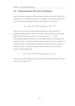
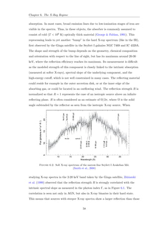
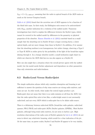
1.3.2 Quasars and QSOs
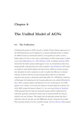
The terms Quasar (Quasi Stellar Radio Source) and QSO (Quasi Stellar Object), often
used interchangeably, are scaled up versions of a Type I Seyfert, where the nucleus has
a luminosity MB 21:5 + 5 log h0 Schmidt Green (1983). Maarten Schmidt
recognized that the pattern of the broad emission lines of 3C 273 (the

43. rst detected
quasar) was the same as the pattern of the Balmer lines of Hydrogen, but were
severely redshifted to z = 0.158 to unfamiliar wavelengths, thus alluding astronomers
from understanding it.
3

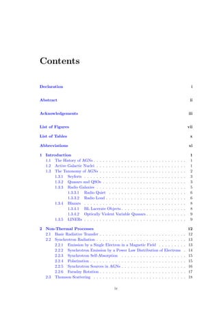
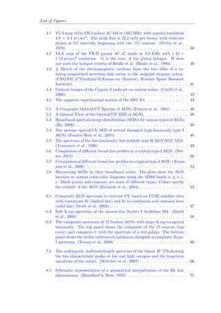
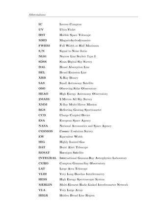
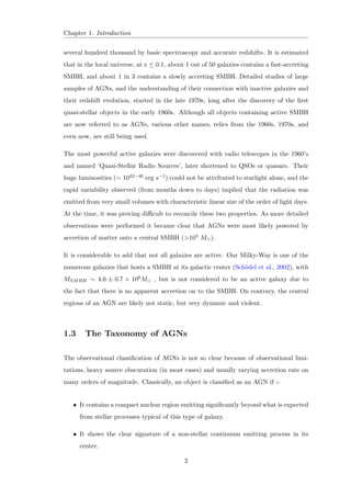
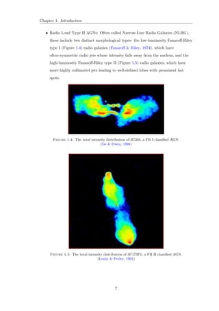
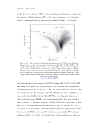
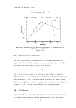
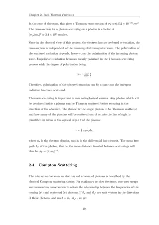
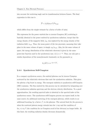
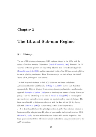
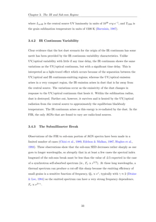
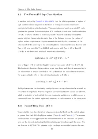
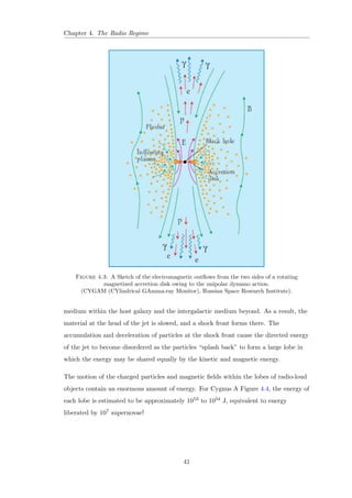
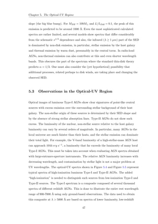
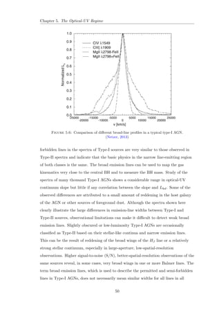
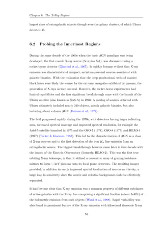
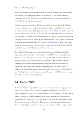
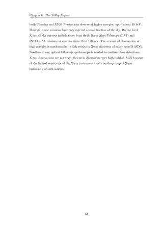
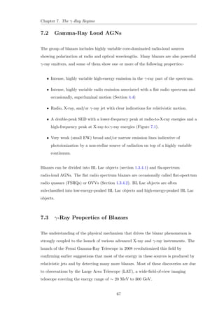
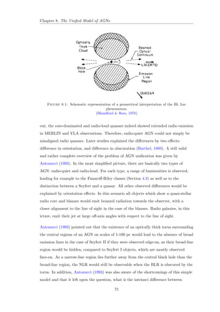
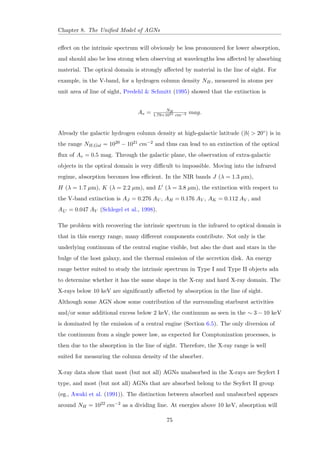
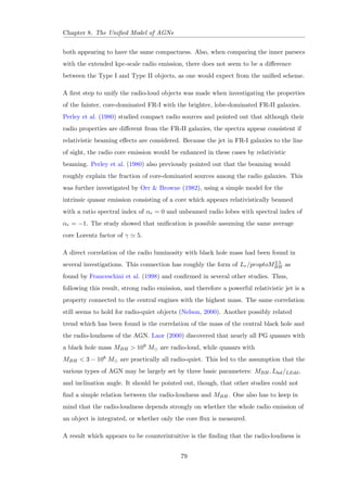
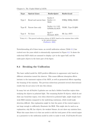
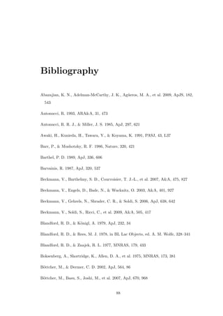
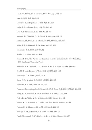
44. Chapter 1. Introduction
Figure 1.1: The spectrum of NGC 1275. The emission features seen at 5057 A
and
6629 A
are [O III] 5007 and H, respectively.
(Sabra et al., 2000)
Figure 1.2: The visible spectrum of Mrk 1157, a Seyfert 2 galaxy.
(Osterbrock, 1984)
4

45. Chapter 1. Introduction
In 1963, the Dutch astronomer Maarten Schmidt recognized that the pattern of the
broad lines of 3C 273 was the same as the pattern of the Balmer lines of Hydrogen,
only severely redshifted to z = 0:158, hence alluding astronomers from identifying its
spectrum. The continuous spectrum of a quasar may span nearly 15 orders of
magnitude in frequency, very broad compared with the sharply peaked blackbody
spectrum of a star. Quasars emit an excess of UV light relative to stars and so are
quite blue in appearance. This UV excess is indicated by the big blue bump in
(nearly) every quasar spectrum. A quasar's radio emission may come either from radio
lobes or from a central source in its core.
Figure 1.3: The visible spectrum of 3C 273, a Quasar.
(Francis et al., 1991)
1.3.3 Radio Galaxies
These galaxies are very luminous at radio wavelengths, with luminosities up to 1039 W
between 10 MHz and 100 GHz. The observed structure in radio emission is determined
by the interaction between twin jets and the external medium, modi

46. ed by the eects
of relativistic beaming. These are further subdivided into two categories.
5

47. Chapter 1. Introduction
1.3.3.1 Radio Quiet
Similar in many aspects to Type I Seyferts, these galaxies show both broad and narrow
lines, the only dierence being that they are much more luminous than Type I
Seyferts. They are observed in the absence of relativistic jets, which contribute the
most energies in the radio wavelength spectrum.
Radio Quiet Type I AGNs: These have relatively low-luminosities and therefore
are seen only nearby, where the host galaxy can be resolved, and the
higher-luminosity radio-quiet quasars, which are typically seen at greater
distances because of their relative rarity locally and thus rarely show an obvious
galaxy surrounding the bright central source.
Radio Quiet Type II AGNs: These include Seyfert II galaxies at low luminosities,
as well as the narrow-emission-line X-ray galaxies (Mushotzky, 1982). The
high-luminosity counterparts are not clearly identi

48. ed at this point but likely
candidates are the infrared-luminous IRAS AGN (Hough et al., 1991, Sanders
et al., 1989, Wills et al., 1992), which may show a predominance of Type II
optical spectra.
1.3.3.2 Radio Loud
Usually attributed to AGNs with unipolar/bipolar, relativistic jets beaming out of
their centers, the radio emission from radio-loud active galaxies is synchrotron
emission, as inferred from its very smooth, broad-band nature and strong polarization.
This implies that the radio-emitting plasma contains, at least, electrons with
relativistic speeds (Lorentz factors of 104) and magnetic

49. elds. However,
synchrotron radiation not being unique to radio wavelengths, if the radio source can
accelerate particles to high enough energies, features which are detected in the radio
may also be seen in the infrared, optical, ultraviolet or even X-ray.
Radio Loud Type I AGNs: These are called Broad-Line Radio Galaxies (BLRG)
at low luminosities and radio-loud quasars at high luminosities, either Steep
Spectrum Radio Quasars (SSRQ) or Flat Spectrum Radio Quasars (FSRQ)
depending on radio continuum shape.
6

50. Chapter 1. Introduction
Radio Loud Type II AGNs: Often called Narrow-Line Radio Galaxies (NLRG),
these include two distinct morphological types: the low-luminosity Fanaro-Riley
type I (Figure 1.4) radio galaxies (Fanaro Riley, 1974), which have
often-symmetric radio jets whose intensity falls away from the nucleus, and the
high-luminosity Fanaro-Riley type II (Figure 1.5) radio galaxies, which have
more highly collimated jets leading to well-de

51. ned lobes with prominent hot
spots.
Figure 1.4: The total intensity distribution of 3C 338, a FR I classi

52. ed AGN.
(Ge Owen, 1994)
Figure 1.5: The total intensity distribution of 3C 173P1, a FR II classi

53. ed AGN.
(Leahy Perley, 1991)
7

54. Chapter 1. Introduction
1.3.4 Blazars
Originally named after what was thought to be an irregular, variable star BL Lacertae,
these are AGNs which are characterized by rapid and large-amplitude
ux variability
and signi

55. cant optical polarization. When compared to quasars with strong emission
lines, blazars have spectra dominated by a featureless non-thermal continuum. The
most well known object in this class is the BL Lacertae. Joining the BL Lac objects in
the blazar classi

56. cation are the optically violently variable quasars (OVVs), which are
similar to the BL Lacs except that they are typically much more luminous, and their
spectra may display broad emission lines. Blazars are AGNs viewed head on and hence
often have jets associated with them (Figure 1.6)
Figure 1.6: The X-ray image of 3C 273's jet.
(3C273 Chandra by Chandra X-ray Observatory - NASA. Licensed under Public
domain via Wikimedia Commons)
1.3.4.1 BL Lacerate Objects
BL Lacertae Objects, or BL Lacs for short, are a subclass of blazars that are
characterized by their rapid time-variability. Their luminosities may change by upto
30% in just 24 hours and by a factor of 100 over a longer time period. BL Lacs are also
distinguished by their strongly polarized power-law continua (30% 40% linear
polarization) that are nearly devoid of emission lines, suggesting that there are very
powerful EM

57. elds at play. BL Lacs, like quasars, are at cosmological distances. Of all
the BL Lacs that have been resolved, 90% of those appear to reside in elliptical
galaxies.
8

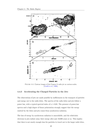
58. Chapter 1. Introduction
1.3.4.2 Optically Violent Variable Quasars
Almost similar to BL Lacs, OVVs are typically much more luminous and may display
broad emission lines in their spectra. The currently best known example of an OVV is
3C 279.
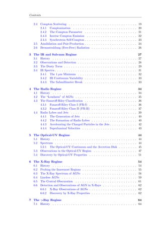
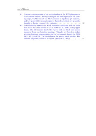
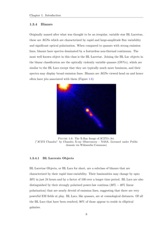
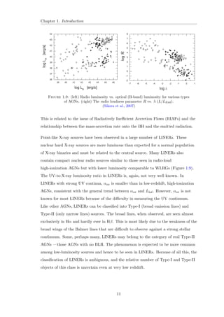
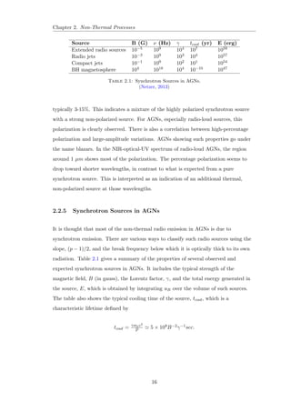
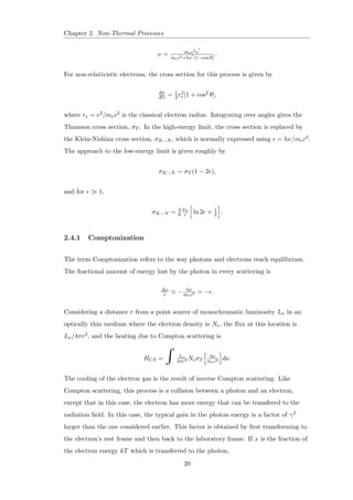
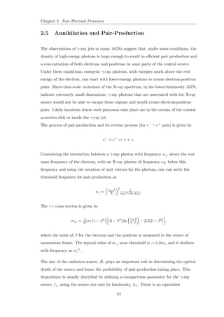
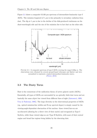
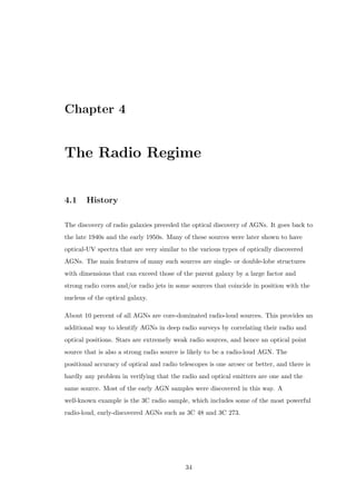
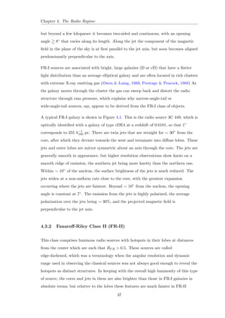
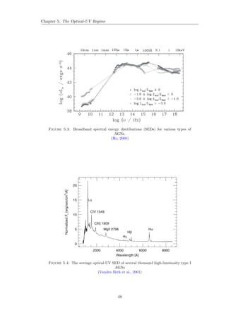
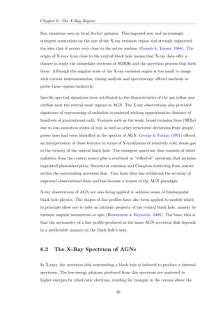
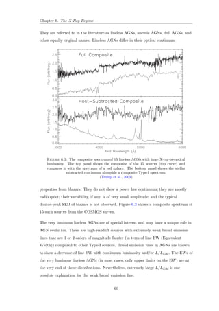
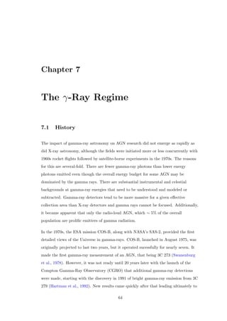
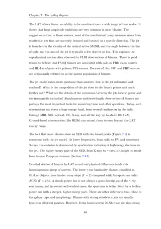
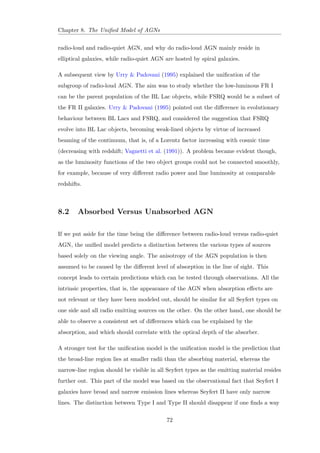
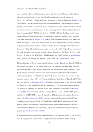
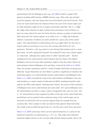
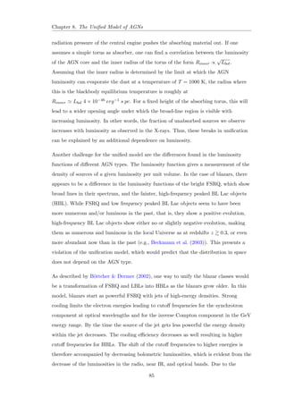
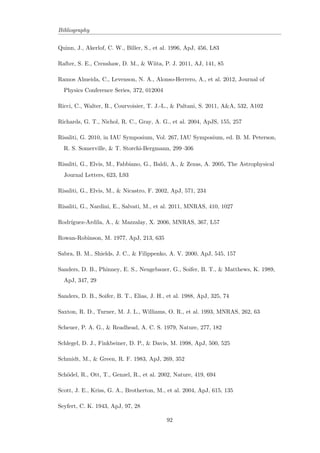
1.3.5 LINERs
LINERs (Low Ionization Nuclear Emission-line Regions) are types of active galaxies
that have very low luminosities in their nuclei, but with fairly strong emission lines of
low-ionization species, such as the forbidden lines of [O I] and [N II]. The Spectra of
LINERs seem similar to the low-luminosity end of the Seyfert II class, and LINER
signatures are detected in many (most of) spiral galaxies in high-sensivity studies.
These low-ionization lines are also detectable in starburst galaxies and in H II regions
and hence it is sometimes dicult to distinguish between LINERs and starburst
galaxies. In the local universe, they are found in about one-third of all galaxies brighter
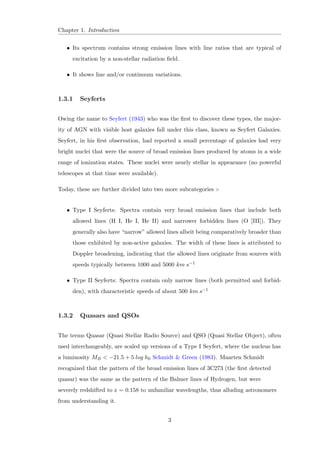
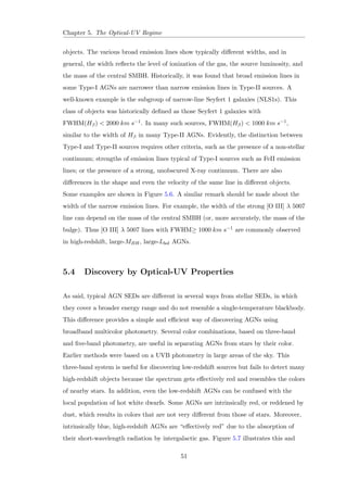
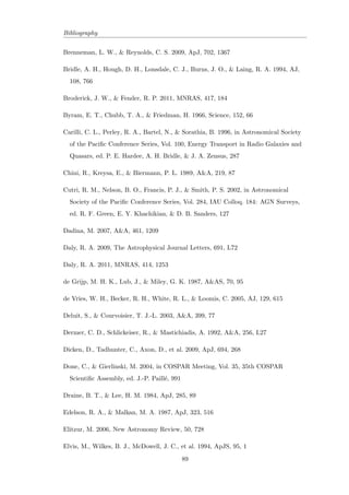
Figure 1.7: The UV spectrum of NGC 4594 LINER observed using the HST FOS.
(Nicholson et al., 1998)
than B = 15.5 mag. This is larger than the number of local high-ionization AGNs by a
factor of 10 or more. Local high-ionization AGNs and LINERs are present in galaxies
with similar bulge luminosities and sizes, neutral hydrogen gas (H I) contents, optical
colors, and stellar masses. Given a certain galaxy type and stellar mass, LINERs are
9

59. Chapter 1. Introduction
usually the lowest-luminosity AGNs, with nuclear luminosity that can be smaller than
the luminosity of high-ionization AGNs by 1-5 orders of magnitude. An alternative
name for this class of objects is low-luminosity AGNs (LLAGNs). The strongest
Figure 1.8: The spread of emission-line galaxies from the SDSS on one diagnostic
diagram that uses four strong optical emission lines, H, H

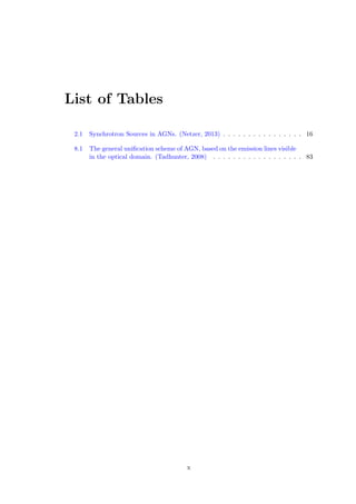
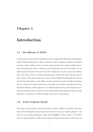
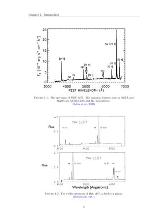
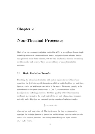
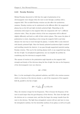
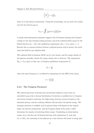
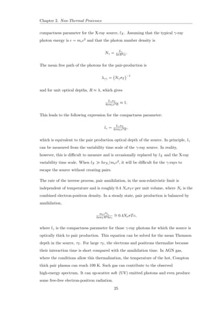
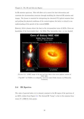
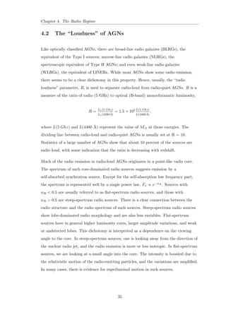
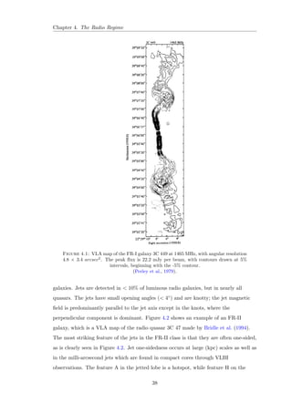
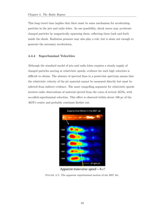
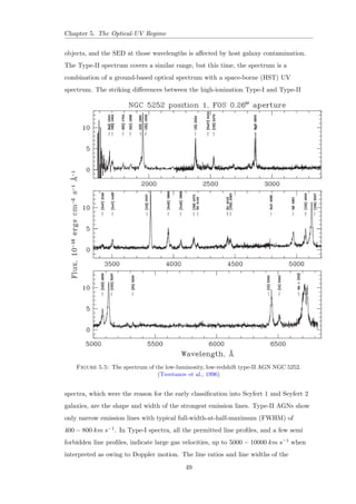
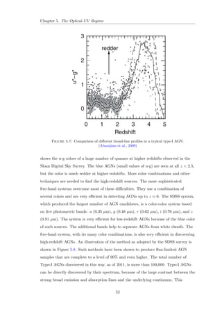
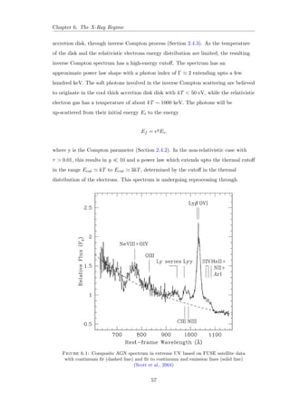
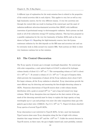
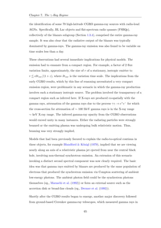
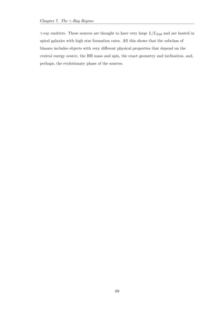
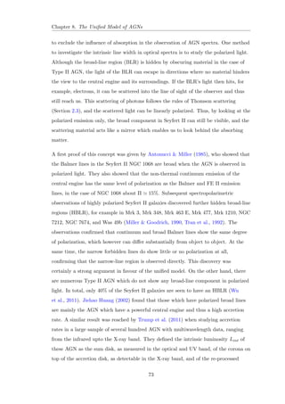
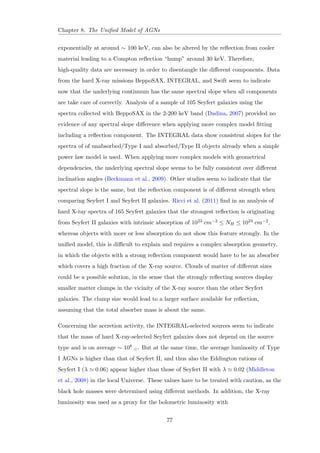
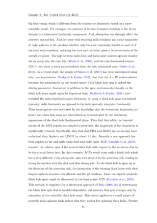
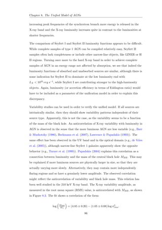
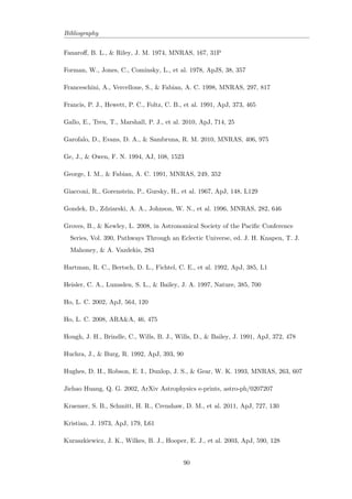
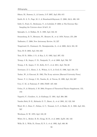
60. , [O III] 5007, and [N
II] 6584, to distinguish galaxies that are dominated by ionization from young stars
(green points) from those that are ionized by a typical AGN SED (blue points for high-ionization
AGNs and red points for low-ionization AGNs). The AGN and SF groups
are well separated, but the division between the two AGN groups is less clear. The
curves indicate empirical (solid) and theoretical (dashed) dividing lines between AGNs
and star-forming galaxies.
(Groves Kewley, 2008)
optical emission lines in the spectrum of LINERs include [O III] 5007, [O II] 3727,
[O I] 6300, [N II] 6584, and hydrogen Balmer lines. All these lines are prominent
also in high-ionization AGNs, but in LINERS, their relative intensities indicate a lower
mean ionization state. For example, the [O III] 5007/H

61. line ratio in LINERs is 3-5
times smaller than in high-ionization Type-II AGNs. Line diagnostic diagrams are
ecient tools to separate LINERs from high-ionization AGNs. One such example is
shown in Figure 1.8. The exact shape of a LINERs SED is still an open issue. In some
sources, it is well represented by the SED shown in Figure 5.3. Such an SED has a
clear de

62. cit at UV wavelengths compared with the spectrum of high-ionization AGNs.
However, some LINERs show strong UV continua and, occasionally, UV continuum
variations, and it is not entirely clear what fraction of the population they represent.
10

63. Chapter 1. Introduction
Figure 1.9: (left) Radio luminosity vs. optical (B-band) luminosity for various types
of AGNs. (right) The radio loudness parameter R vs. (L=LEdd).
(Sikora et al., 2007)
This is related to the issue of Radiatively Inecient Accretion Flows (RIAFs) and the
relationship between the mass-accretion rate onto the BH and the emitted radiation.
Point-like X-ray sources have been observed in a large number of LINERs. These
nuclear hard X-ray sources are more luminous than expected for a normal population
of X-ray binaries and must be related to the central source. Many LINERs also
contain compact nuclear radio sources similar to those seen in radio-loud
high-ionization AGNs but with lower luminosity comparable to WLRGs (Figure 1.9).
The UV-to-X-ray luminosity ratio in LINERs is, again, not very well known. In
LINERs with strong UV continua, ox is smaller than in low-redshift, high-ionization
AGNs, consistent with the general trend between ox and Lbol. However, ox is not
known for most LINERs because of the diculty in measuring the UV continuum.
Like other AGNs, LINERs can be classi

64. ed into Type-I (broad emission lines) and
Type-II (only narrow lines) sources. The broad lines, when observed, are seen almost
exclusively in H and hardly ever in H

65. . This is most likely due to the weakness of the
broad wings of the Balmer lines that are dicult to observe against a strong stellar
continuum. Some, perhaps many, LINERs may belong to the category of real Type-II
AGNs |those AGNs with no BLR. The phenomenon is expected to be more common
among low-luminosity sources and hence to be seen in LINERs. Because of all this, the
classi

66. cation of LINERs is ambiguous, and the relative number of Type-I and Type-II
objects of this class is uncertain even at very low redshift.
11

67. Chapter 2
Non-Thermal Processes
Much of the electromagnetic radiation emitted by AGNs is very dierent from a simple
blackbody emission or a stellar radiation source. The general name adopted here for
such processes is non-stellar emission, but the term non-thermal emission is commonly
used to describe such sources. There are several types of non-stellar radiation
processes.
2.1 Basic Radiative Transfer
Describing the interaction of radiation with matter requires the use of three basic
quantities: the

68. rst is the speci

69. c intensity I, which gives the local
ux per unit time,
frequency, area, and solid angle everywhere in the source. The second quantity is the
monochromatic absorption cross section, (cm1), which combines all loss
(absorption and scattering) processes. The third quantity is the volume emission
coecient, j, which gives the locally emitted
ux per unit volume, time, frequency,
and solid angle. The three are combined into the equation of radiative transfer,
dI
ds = I + j;
where ds is a path length interval. The

70. rst term on the right in this equation
describes the radiation loss due to absorption, and the second gives the radiation gain
due to local emission processes. One usually de

71. nes the optical depth element,
d = ds. Hence,
12

72. Chapter 2. Non-Thermal Processes
dI
d
= I + S;
where S = j= is the source function. The formal solution of the equation of
transfer depends on geometry. For a slab of thickness in a direction perpendicular
to the slab, it is
I() = I(0)e +
R
0
e(t)S(t)dt:
For any other direction , both and dt must be divided by cos .
The general equation of radiative transfer is dicult to solve and requires numerical
techniques. However, there are simple cases in which the solution is straightforward.
In particular, the case of a slab and a constant source function that is independent of
allows a direct integration and gives the following solution:
I = I(0)e + S(1 e ):
For an opaque source in full thermodynamic equilibrium (TE), the optical depth is
large, and both I and S approach the Planck function
B(T) = 2h3=c2
eh=kT1
2.2 Synchrotron Radiation
2.2.1 Emission by a Single Electron in a Magnetic Field
Considering an electron of energy E that is moving in a uniform magnetic

73. eld B of
energy density uB = B2=8, the energy loss rate, dE=dt, which is also the power
emitted by the electron, P, is given by
P = 2T c
2

74. 2uB sin2 ;
where T is the Thomson cross section,
c is the speed of light,
13

75. Chapter 2. Non-Thermal Processes
= E=mc2 is the Lorentz factor,

76. = v=c, and
v is the speed of the electron.
The angular term sin2 re
ects the direction of motion, where is the pitch angle
between the direction of the motion and the magnetic

77. eld. Averaging over isotropic
pitch angles gives
P = (4=3)T c
2

78. 2uB:
The radiation emitted by a single electron is beamed in the direction of motion. The
spectral energy distribution (SED) of this radiation is obtained by considering the gyro
frequency of the electrons around the

79. eld lines (!B = eB=
mec) and the mean interval
between pulses (2=!B). The calculation of the pulse width is obtained by considering
the relativistic time transformation between the electron frame and the observer frame.
This involves an additional factor of
2. Thus, the pulse width is proportional to
3
or, expressed with the Larmor angular frequency, !L = eB=mec (which diers from !B
by a factor of
), to
2. Fourier transforming these expressions gives the mean
emitted spectrum of a single electron, P
, which peaks at a frequency near
2!L.
2.2.2 Synchrotron Emission by a Power Law Distribution of Electrons
Assuming now a collection of electrons with an energy distribution n(
)d
that gives
the number of electrons per unit volume with
in the range
(
+ d
), the emission
coecient due to the electrons is obtained by summing P
(
) over all energies:
j = 1
4
1 R
1
P(
)n(
)d
:
There is no general analytical solution to this expression since n(
) can take various
dierent forms. However, there are several cases of interest where n(
) can be
presented as a power law in energy:
n(
)d
= n0
pd
:
The additional assumption that all the radiation peaks around a characteristic
frequency,
2L, where L is the Larmor frequency, gives the following solution for j:
14

80. Chapter 2. Non-Thermal Processes
3T n0uB1
4j = 2
L
L
p1
2 :
Figure 2.1: A comparison of a synchrotron source with p = 2:5 (solid line) and a 105
K blackbody source (dotted line).
(Netzer, 2013)
2.2.3 Synchrotron Self-Absorption
The source of fast electrons can be opaque to its own radiation. This results in a
signi

81. cant modi

82. cation of the emergent spectrum especially at low frequencies, where
the opacity is the largest. It can be shown that in this case,
/ p+4
2 ;
that is, the largest absorption is at the lowest frequencies. Using the equation of
radiative transfer for a uniform homogeneous medium, we get the solution at the large
optical depth limit, I / 5=2, which describes the synchrotron SED at low energies.
This function drops faster toward low energies than the low-energy drop of a blackbody
spectrum (I / 2). The overall shape of such a source is shown in Figure 2.1.
2.2.4 Polarization
Synchrotron radiation is highly linearly polarized. The intrinsic polarization can reach
70%. However, what is normally observed is a much smaller level of polarization,
15

83. Chapter 2. Non-Thermal Processes
Source B (G) (Hz)
tcool (yr) E (erg)
Extended radio sources 105 109 104 107 1059
Radio jets 103 109 103 104 1057
Compact jets 101 109 102 101 1054
BH magnetosphere 104 1018 104 1010 1047
Table 2.1: Synchrotron Sources in AGNs.
(Netzer, 2013)
typically 3-15%. This indicates a mixture of the highly polarized synchrotron source
with a strong non-polarized source. For AGNs, especially radio-loud sources, this
polarization is clearly observed. There is also a correlation between high-percentage
polarization and large-amplitude variations. AGNs showing such properties go under
the name blazars. In the NIR-optical-UV spectrum of radio-loud AGNs, the region
around 1 m shows most of the polarization. The percentage polarization seems to
drop toward shorter wavelengths, in contrast to what is expected from a pure
synchrotron source. This is interpreted as an indication of an additional thermal,
non-polarized source at those wavelengths.
2.2.5 Synchrotron Sources in AGNs
It is thought that most of the non-thermal radio emission in AGNs is due to
synchrotron emission. There are various ways to classify such radio sources using the
slope, (p 1)=2, and the break frequency below which it is optically thick to its own
radiation. Table 2.1 gives a summary of the properties of several observed and
expected synchrotron sources in AGNs. It includes the typical strength of the
magnetic

84. eld, B (in gauss), the Lorentz factor,
, and the total energy generated in
the source, E, which is obtained by integrating uB over the volume of such sources.
The table also shows the typical cooling time of the source, tcool, which is a
characteristic lifetime de

85. ned by
tcool =
mec2
P
' 5 108B2
1sec:
16

86. Chapter 2. Non-Thermal Processes
2.2.6 Faraday Rotation
Michael Faraday discovered in 1845 that the angle of polarization of an
electromagnetic wave changes when the wave is sent through a medium with a
magnetic

87. eld. The so-called Faraday rotation can also aect the synchrotron
emission. Faraday rotation can be understood as the dierent eect the magnetized
plasma has on the left and right circularly polarized light. Depending on the
orientation with respect to the magnetic

88. eld, the components will see a dierent
refractive index. Thus, the phase velocity of the two components will be aected
slightly dierently and lead to a shift of their relative phases. This causes the plane of
polarization to rotate, depending on how strong the magnetic

89. eld is and what
distance the wave has to travel through the plasma. A similar eect is also observed
with linearly polarized light. Once the linearly polarized synchrotron light is emitted
and travelling towards the observer, it can pass through magnetized material causing
Faraday rotation. This can be the emitting plasma itself, or any magnetized gas along
the line of sight. In astrophysical applications, one can simplify the problem by
considering only free electrons in magnetic

90. elds.
The amount of rotation in the polarization angle depends on the magnetic

91. eld
strength and density of the electrons along the line of sight, but also on the frequency
of the electromagnetic wave one observes:
= 2RM:
Here, is the wavelength of the polarized radiation, and RM is the rotation measure
which is a function of the electron density ne and of the component of the magnetic

92. eld Bjj parallel to the line of sight:
= 2 e3
2m2c4
R
ne(s)Bjj(s)ds:
Thus, the rotation is larger for low frequencies. This is because the frequency of the
wave is much larger than the gyro-frequency of the electron. The closer the light and
the electron are to a resonant state, and thus the larger the energy transfer from the
wave to the electron. The light from extragalactic sources will not only have to cross
the intergalactic medium, but the interstellar medium of our galaxy as well on its path
17

93. Chapter 2. Non-Thermal Processes
to the observer. The magnetic

94. eld along the line of sight will not be constant, and
importantly, it will not be of the same orientation throughout the path of light. To
determine the net eect of Faraday rotation, it is necessary to measure polarization at
closely spaced frequency interval over many frequencies. Because the rotation aects
the high frequency the least, the best way to get an estimate of the intrinsic
polarization of a synchrotron source is to measure at high frequencies.
2.3 Thomson Scattering
Thomson scattering describes the non-relativistic case of an interaction between an
electromagnetic wave and a free charged particle. The eect was

95. rst describe by Sir
Joseph John Thomson, who discovered the electron when studying cathode rays in the
late nineteenth century. The process can be understood as elastic or coherent
scattering, as the photon and the particle will have the same energy after the
interaction as before. For this process of the energy E of the photon has to be much
smaller than the rest energy of the particle:
E = h mc2:
Another requirement for Thomson scattering is that the particle must be moving at
non-relativistic speed (v c). In the classical view of this process, the incoming
photon is absorbed by the particle with charge q, which is set into motion and then
re-emits a photon of the same energy.
Using the classical electron radius r0 = q2=mc2 (Bohr radius), the dierential
cross-section of this elastic scattering process can be written as
d
d
= 1
2(1 + cos2 )r2
0:
This is symmetric with respect to the angle , thus the amount of radiation scattered
in the forward and backward direction is equal. The total cross-section is then given by
T = 2
R
0
d
d
sin d = 8
3 r2
0 = 8
3
q2
mc2
2
:
18

96. Chapter 2. Non-Thermal Processes
In the case of electrons, this gives a Thomson cross-section of T ' 6:652 1025 cm2.
The cross-section for a photon scattering on a photon is a factor of
(mp=me)2 ' 3:4 106 smaller.
Since in the classical view of this process, the electron has no preferred orientation, the
cross-section is independent of the incoming electromagnetic wave. The polarization of
the scattered radiation depends, however, on the polarization of the incoming photon
wave. Unpolarized radiation becomes linearly polarized in the Thomson scattering
process with the degree of polarization being
= 1cos2
1+cos2 :
Therefore, polarization of the observed emission can be a sign that the emergent
radiation has been scattered.
Thomson scattering is important in may astrophysical sources. Any photon which will
be produced inside a plasma can be Thomson scattered before escaping in the
direction of the observer. The chance for the single photon to be Thomson scattered
and how many of the photons will be scattered out of or into the line of sight is
quanti

97. ed in terms of the optical depth of the plasma:
=
R
T nedx;
where ne is the electron density, and dx is the dierential line element. The mean free
path T of the photon, that is, the mean distance traveled between scatterings will
thus be T = (T ne)1.
2.4 Compton Scattering
The interaction between an electron and a beam of photons is described by the
classical Compton scattering theory. For stationary or slow electrons, one uses energy
and momentum conservation to obtain the relationship between the frequencies of the
coming (
0
) and scattered () photons. If ~n and ~n0 are unit vectors in the directions
of these photons, and cos = ~n ~n0 , we get
19

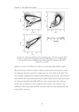
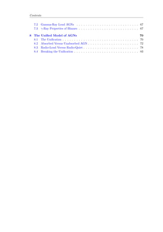
98. Chapter 2. Non-Thermal Processes
= mec2
0
mec2+h0 (1cos )
:
For non-relativistic electrons, the cross section for this process is given by
d
d
= 1
2r2
e [1 + cos2 ];
where re = e2=mec2 is the classical electron radius. Integrating over angles gives the
Thomson cross section, T . In the high-energy limit, the cross section is replaced by
the Klein-Nishina cross section, KN, which is normally expressed using = h=mec2.
The approach to the low-energy limit is given roughly by
KN T (1 2);
and for 1,
KN 3
8
T
h
ln 2 + 1
2
i
:
2.4.1 Comptonization
The term Comptonization refers to the way photons and electrons reach equilibrium.
The fractional amount of energy lost by the photon in every scattering is
' h
mec2 = :
Considering a distance r from a point source of monochromatic luminosity L in an
optically thin medium where the electron density is Ne, the
ux at this location is
L=4r2, and the heating due to Compton scattering is
HCS =
R
L
4r2NeT
h
h
mec2
i
d:
The cooling of the electron gas is the result of inverse Compton scattering. Like
Compton scattering, this process is a collision between a photon and an electron,
except that in this case, the electron has more energy that can be transfered to the
radiation

99. eld. In this case, the typical gain in the photon energy is a factor of
2
larger than the one considered earlier. This factor is obtained by

100. rst transforming to
the electron's rest frame and then back to the laboratory frame. If x is the fraction of
the electron energy kT which is transferred to the photon,
20

101. Chapter 2. Non-Thermal Processes
*
+
= x kTe
mec2 ;
where Te is the electron temperature. Using this terminology, one can write the cooling
term for the electron gas as
CCS =
R
L
4r2NeT
h
xkTe
mec2
i
d:
A simple thermodynamical argument suggests that if Compton heating and Compton
cooling are the only heating-cooling processes, and if the radiation

102. eld is given by the
Planck function (L = B), the equilibrium requirement, HCS = CCS, gives x = 4.
Because this is a general relation between a physical process and its inverse, the result
must also hold for any radiation

103. eld.
The radiation

104. eld in luminous AGNs can be very intense, and the energy density of
the photons normally exceeds the energy density due to electrons. The requirement
HCS = CCS gives, in this case, a Compton equilibrium temperature of
TC = h
4k ;
where the mean frequency, , is de

105. ned by integrating over the SED of the source,
=
R
RLd
Ld :
2.4.2 The Compton Parameter
The emitted spectrum of thermal and non-thermal radiation sources that are
embedded in gas with a thermal distribution of velocities is modi

106. ed due to Compton
and inverse Compton scattering. For high-energy electrons, inverse Compton is the
dominant process, and the resulting collisions will up-scatter the photon energy. The
emergent spectrum is modi

107. ed, and its spectral shape will depend on the original
shape, the electron temperature, and the Compton depth of the source, which
determines the number of scattering before escape. Considering an initial photon
energy of hi and the case of thermal electrons with temperature Te such that
hi 4kTe, the scattering of such photons by a fast electron will result in energy gain
21