The document describes the design of an afterburning low bypass turbofan engine to replace the General Electric J85 engine used on the Northrop Grumman T-38 Talon jet trainer. Initial values were obtained through parametric analysis in AEDsys ONX. A low bypass twin spool compressor with 3 fan stages and 5 high pressure compressor stages was selected. Additional components including the combustion chamber, turbines, and convergent-divergent nozzle were designed. The final engine design met the criteria of reduced thrust specific fuel consumption and weight while maintaining required thrust.

1. i
DKA-867
David Byrd
Kristian Lien
Austin Sims
Kennesaw State University
SYE 4803
Spring 2016

2. ii
Abstract
The American Institute of Aeronautics and Astronautics created an engine design competition to be
obtained via a student body. The objective was to design an afterburning low bypass turbofan engine to
replace the General Electric-J85-5A afterburning turbojet engine used on the Northrop Grumman T-38
Talon trainer jet. The new engine is required to have a lower thrust specific fuel consumption, weight, and
improved thrust while maintaining current performance characteristics.
By completing multiple parametric analysis, via the AEDsys ONX program, initial values were obtained for
the design of the engine. The initial input values of the parametric analysis were based on the given
baseline engine. Initially, an inlet had to be designed at the harshest flight condition. The condition given
to us was at a Mach number of 1.3. After obtaining a fan inlet Mach low enough not to cause structural
damage, the number of fan and high pressure compressor stage had to be found. A low bypass twin spool
compressor was selected to reduce the weight and achieve the required thrust. Multiple iterations with
various stages were conducted and finalized to be a total of three fan stages and five high pressure
compressor stages. The compressor was then designed to allow for both increase in pressure and
decrease in flow velocity so that the combustion chamber would not flame out and provide significant
efficiency. The combustion chamber was next on the design agenda. A diffuser was developed along with
cooling flow and number of nozzles to obtain complete combustion. Both a high pressure and low
pressure turbine was then designed based on the given temperature output and power needed to drive
both fan and high pressure compressor. An afterburner was then developed to obtain the needed
supersonic specification. The afterburner uses both the bypass and core exit streams to increase the
propulsive efficiency. In order to produce enough thrust and a high enough exit velocity, a convergent-
divergent nozzle was designed. Ultimately, at the takeoff flight condition the nozzle releases a gross thrust
of 3,981 pound-force at the exit. Combined with a second engine, this will be sufficient thrust at takeoff
for the given aircraft. Upon completion of the engine design, it was found that both takeoff and cruise
thrust specific fuel consumption was reduced to: 1.954 pound-mass-per-hour-per-pound-force and 1.807
pound-mass-per-hour-per-pound-force. By maintaining a fan diameter of twenty inches, the overall
length was less than 108.1 inches, and the weight without tailpipe was less than 584 pounds; the design
criteria was met. Each of these results were found using fifth generation designs and materials.

3. iii
Table of Contents
List of Figures.....................................................................................................................................v
List of Tables...................................................................................................................................viii
Nomenclature...................................................................................................................................ix
1 Introduction ...............................................................................................................................1
1.1 Justification.........................................................................................................................1
1.2 Problem Statement.............................................................................................................1
2 Gas Turbine Engine Components.................................................................................................1
2.1 Inlet....................................................................................................................................2
2.2 Compressor.........................................................................................................................2
2.3 Combustion Chamber..........................................................................................................3
2.4 Turbine...............................................................................................................................4
2.5 Afterburner.........................................................................................................................4
2.6 Nozzle.................................................................................................................................4
3 Problem Solving Approach..........................................................................................................5
3.1 Requirement.......................................................................................................................5
3.2 Gantt Chart.........................................................................................................................7
3.3 Flow Charts.........................................................................................................................7
3.4 Project Management...........................................................................................................8
3.5 Responsibilities ................................................................................................................9
3.6 Cost Analysis.......................................................................................................................9
3.7 Resources Available & Used.................................................................................................9
4 Results and Discussion..............................................................................................................10
4.1 Parametric Analysis...........................................................................................................10
4.2 AEDsys Software Analysis..................................................................................................13
4.2.1 Inlet .....................................................................................................................................14
4.2.2 Fan & Compressor...............................................................................................................18
4.2.3 Combustion Chamber .........................................................................................................21
4.2.4 Turbine................................................................................................................................26
4.2.5 Afterburner .........................................................................................................................31
4.2.6 Nozzle..................................................................................................................................32
4.3 Weight Calculation Method...............................................................................................34
4.4 Mission Analysis................................................................................................................34
4.5 Results..............................................................................................................................35
4.5.1 Compliance Matrix..............................................................................................................36
4.5.2 Engine Summary Data.........................................................................................................37
4.5.3 Required Detailed Stage and Component Information ......................................................39
4.5.4 Velocity Triangles................................................................................................................41
5 Material Selections...................................................................................................................45
5.1 Aluminum 2124 Alloy (ρ = 5.29 slug/ft3
).............................................................................45
5.2 Titanium 6246 Alloy (ρ = 9.08 slug/ft3
) ...............................................................................46
5.3 Inconel 601 (ρ = 15.6 slug/ft3
) ............................................................................................47
5.4 Hastelloy X (ρ = 16.0 slug/ft3
).............................................................................................48
5.5 Rene’ 80 (ρ = 15.9 slug/ft3
) ................................................................................................49

4. iv
6 Conclusion................................................................................................................................51
7 References ...............................................................................................................................52
8 Appendix A: Acknowledgements ............................................................................................53
9 Appendix B: Contact Information ...........................................................................................54
10 Appendix C: Reflections ......................................................................................................55
11 Appendix D: Initial Values and Requirements ........................................................................58
11.1 Inlet..................................................................................................................................58
11.2 Fan/Compressor................................................................................................................58
11.3 Combustion Chamber........................................................................................................59
11.4 Turbine.............................................................................................................................59
11.5 Afterburner.......................................................................................................................60
11.6 Nozzle...............................................................................................................................61
12 Appendix E: ONX Parametric Analysis....................................................................................64
12.1 Mach 0 and Sea Level ........................................................................................................64
12.2 Mach 0.5 and 15,000 feet ..................................................................................................66
12.3 Mach 0.85 and 35,000 feet ................................................................................................68
12.4 Mach 1.3 and 40,000 feet ..................................................................................................70
13 Appendix F: AEDsys Test Data ...............................................................................................72
13.1 Inlet..................................................................................................................................72
13.2 Fan/Compressor................................................................................................................73
13.2.1 Inlet Guide Vanes................................................................................................................73
13.2.2 Fan/Low Pressure Compressor ...........................................................................................75
13.2.3 High Pressure Compressor..................................................................................................78
13.3 Combustion Chamber........................................................................................................84
13.4 Turbine.............................................................................................................................88
13.4.1 High Pressure Turbine.........................................................................................................88
13.4.2 Low Pressure Turbine..........................................................................................................89
13.4.3 Exit Guide Vanes .................................................................................................................90
13.5 Afterburner.......................................................................................................................91
13.6 Nozzle...............................................................................................................................92
13.6.1 Mach 0.................................................................................................................................92
13.6.2 Mach 0.5 .............................................................................................................................93
13.6.3 Mach 0.85 ...........................................................................................................................94
13.6.4 Mach 1.3 .............................................................................................................................94
13.7 Mission Analysis Results....................................................................................................95

5. v
List of Figures
Figure 2.1: Cutaway of an Axial-flow Compressor........................................................................................3
Figure 3.1: Gantt Chart for Overall Project...................................................................................................7
Figure 3.2: Overall Project Flow Chart ..........................................................................................................8
Figure 3.3: Flow Chart for Responsibilities ...................................................................................................9
Figure 4.1: Low Bypass Turbofan Station Numbering.................................................................................10
Figure 4.2: External compression inlet .......................................................................................................14
Figure 4.3: Shock Pressure Recovery for Freestream Mach Number and Number of Oblique Shocks......15
Figure 4.4: Multi Shock Compression for Oswatisch Optimization ............................................................15
Figure 4.5: CAD of First Stage Low Pressure Fan Blade ..............................................................................21
Figure 4.6: Operating regimes ....................................................................................................................22
Figure 4.7: Geometry of flat-wall diffuser ..................................................................................................22
Figure 4.8: Geometry of dump diffuser ......................................................................................................22
Figure 4.9: Geometry of combined diffuser ...............................................................................................22
Figure 4.10: CAD of the High Pressure Turbine Blade ................................................................................30
Figure 4.11: Turbine Transpiration and Full-Coverage Film Cooling...........................................................31
Figure 4.12: Geometry of Afterburner........................................................................................................32
Figure 4.13: Flow Patterns in the Afterburner............................................................................................32
Figure 4.14: Principal Features ...................................................................................................................32
Figure 4.15: Nozzle geometric parameters.................................................................................................33
Figure 4.16: Compressor Velocity Triangles................................................................................................41
Figure 4.17: Turbine Velocity Triangle........................................................................................................44
Figure 5.1: Effect of Temperature and Exposure Time on Tensile Properties............................................45
Figure 5.2: Creep and Creep-rupture curves at temperatures from 75 to 600˚F for 2124-T851 plate......46
Figure 5.3: Axial Fatigue Properties of α-β forged materials in two heat-treated conditions ...................46
Figure 5.4: Minimum creep rate at various temperatures and stresses ....................................................47
Figure 5.5: Fatigue properties of annealed sheet.......................................................................................47
Figure 5.6: Creep-deformation curves for plate and bar at temperatures of 1200-1800˚F.......................48
Figure 5.7: Fatigue life of plate at various temperatures in air and impure helium at atmospheric pressure
............................................................................................................................................................48
Figure 5.8: Effect of elevated temperature on modulus of elasticity.........................................................49
Figure 5.9: Creep Strain and creep-rupture at 1400, 1600, and 1800˚F for fully treated cast alloy ..........49
Figure 5.10: Axial Low Cycle Fatigue behavior at 1200-1800˚F ..................................................................50
Figure 11.1: Principal Features and Flow Patterns of the Afterburner.......................................................60
Figure 11.2: Nozzle Discharge Coefficient: b) Convergent and C-D Nozzle CD max...................................61
Figure 11.3: C-D Nozzle Velocity Coefficient...............................................................................................62
Figure 11.4: C-D Nozzle Angularity Coefficient...........................................................................................63
Figure 12.1: ONX Parametric Analysis Results at M=0 and Sea Level.........................................................64
Figure 12.2: Preliminary Engine Performance Analysis at M=0 and Sea Level..........................................65
Figure 12.3: ONX Parametric Results at M=0.5 and 15,000 feet ................................................................66
Figure 12.4: Preliminary Engine Performance Analysis at M=0.5 and 15,000 feet ....................................67
Figure 12.5: ONX Parametric Analysis Results M=0.85 and 35,000 feet ....................................................68
Figure 12.6: Preliminary Engine Performance Analysis at M=0.85 and 35,000 feet ..................................69
Figure 12.7: ONX Parametric Analysis Results at M=1.3 and 40,000 feet..................................................70
Figure 12.8: Preliminary Engine Performance Analysis at M=1.3 and 40,000 feet ....................................71
Figure 13.1: Inlet Inputs and Results ..........................................................................................................72
Figure 13.2: Inlet Side View ........................................................................................................................73

6. vi
Figure 13.3: Inlet Angle Contours ...............................................................................................................73
Figure 13.4: Low Pressure IGV Results........................................................................................................73
Figure 13.5: Low Pressure IGV Blade Profile...............................................................................................74
Figure 13.6: High Pressure IGV Results.......................................................................................................74
Figure 13.7: High Pressure IGV Blade Profile..............................................................................................74
Figure 13.8: Fan/Low Pressure Compressor Layout ...................................................................................75
Figure 13.9: Low Pressure Stage 1 Results..................................................................................................75
Figure 13.10: Low Pressure Stage 1 Blade Profile.......................................................................................76
Figure 13.11: Low Pressure Stage 2 Results................................................................................................76
Figure 13.12: Low Pressure Stage 2 Blade Profiles.....................................................................................77
Figure 13.13: Low Pressure Stage 3 Results................................................................................................77
Figure 13.14: Low Pressure Stage 3 Blade Layout ......................................................................................78
Figure 13.15: High Pressure Compressor Layout........................................................................................78
Figure 13.16: High Pressure Stage 1 Results...............................................................................................79
Figure 13.17: High Pressure Stage 1 Blade Layout......................................................................................79
Figure 13.18: High Pressure Stage 2 Results...............................................................................................80
Figure 13.19: High Pressure Stage 2 Blade Profile......................................................................................80
Figure 13.20: High Pressure Stage 3 Results...............................................................................................81
Figure 13.21: High Pressure Stage 3 Blade Profile......................................................................................81
Figure 13.22: High Pressure Stage 4 Results...............................................................................................82
Figure 13.23: High Pressure Stage 4 Blade Profile......................................................................................82
Figure 13.24: High Pressure Stage 5 Results...............................................................................................83
Figure 13.25: High Pressure Stage 5 Blade Profile......................................................................................83
Figure 13.26: Data Entry for Combustion Chamber....................................................................................84
Figure 13.27: Air Partitioning for Combustion Chamber ............................................................................84
Figure 13.28: Diffuser for Combustion Chamber........................................................................................85
Figure 13.29: Primary Zone for Combustion Chamber...............................................................................85
Figure 13.30: Secondary Zone for Combustion Chamber...........................................................................86
Figure 13.31: Dilution Zone for Combustion Chamber...............................................................................86
Figure 13.32: Combustion Chamber Front View.........................................................................................87
Figure 13.33: Combustion Chamber Side View ..........................................................................................87
Figure 13.34: Combustion Chamber Plan View ..........................................................................................88
Figure 13.35: High Pressure Results............................................................................................................88
Figure 13.36: High Pressure Layout ............................................................................................................89
Figure 13.37: High Pressure Blade Layout ..................................................................................................89
Figure 13.38: Low Pressure Results ............................................................................................................89
Figure 13.39: Low Pressure Layout.............................................................................................................90
Figure 13.40: Low Pressure Blade Layout...................................................................................................90
Figure 13.41: Exit Guide Vane Results ........................................................................................................90
Figure 13.42: Exit Guide Vane Results ........................................................................................................90
Figure 13.43: Data Entry .............................................................................................................................91
Figure 13.44: Data Entry .............................................................................................................................91
Figure 13.45: Flameholders ........................................................................................................................91
Figure 13.46: Side View of Afterburner ......................................................................................................92
Figure 13.47: Nozzle Input and Results at Mach 0......................................................................................92
Figure 13.48: Divergent Angle Contours at Mach 0....................................................................................93
Figure 13.49: Nozzle Side View at Mach 0..................................................................................................93
Figure 13.50: Nozzle Input and Results at Mach 0.5...................................................................................93

7. vii
Figure 13.51: Divergent Angle Contours at Mach 0.5.................................................................................93
Figure 13.52: Nozzle Side View at Mach 0.5...............................................................................................93
Figure 13.53: Nozzle Input and Results at Mach 0.85.................................................................................94
Figure 13.54: Divergent Angle Contours at Mach 0.85...............................................................................94
Figure 13.55: Nozzle Side View at Mach 0.85.............................................................................................94
Figure 13.56: Nozzle Input and Results at Mach 1.3...................................................................................94
Figure 13.57: Divergent Angle Contour at Mach 1.3 ..................................................................................95
Figure 13.58: Nozzle Side View at Mach 1.3...............................................................................................95
Figure 13.59: Warm-Up Leg........................................................................................................................95
Figure 13.60: Takeoff Accelerate ................................................................................................................96
Figure 13.61: Takeoff Rotation ...................................................................................................................96
Figure 13.62: Horizontal Acceleration ........................................................................................................97
Figure 13.63: First Climb and Acceleration.................................................................................................97
Figure 13.64: Second Climb and Acceleration ............................................................................................98
Figure 13.65: Third Climb and Acceleration................................................................................................98
Figure 13.66: Subsonic Cruise.....................................................................................................................99
Figure 13.67: Climb and Accelerate to Supersonic Cruise ..........................................................................99
Figure 13.68: Supersonic Cruise................................................................................................................100
Figure 13.69: Descend to Subsonic Cruise................................................................................................100
Figure 13.70: Subsonic Cruise...................................................................................................................101
Figure 13.71: Descend to Loiter................................................................................................................101
Figure 13.72: Loiter...................................................................................................................................102
Figure 13.73: Descend to Land..................................................................................................................102
Figure 13.74: Results of Mission...............................................................................................................103

8. viii
List of Tables
Table 3.1: Cost Analysis for Engine ...............................................................................................................9
Table 4.1: Compliance Matrix.....................................................................................................................36
Table 4.2: Engine Summary Data................................................................................................................37
Table 4.3: Fan / LP Compressor Flow Station Data.....................................................................................37
Table 4.4: HP Compressor Flow Station Data .............................................................................................38
Table 4.5: Turbine & Nozzle Flow Data.......................................................................................................38
Table 4.6: Additional Information...............................................................................................................38
Table 4.7: Fan / Low Pressure Compressor Detailed Data..........................................................................39
Table 4.8: High Pressure Compressor Detailed Data..................................................................................40
Table 4.9: Turbine Detailed Data ................................................................................................................40
Table 4.10: Fan/Low Pressure Compressor ................................................................................................42
Table 4.11: High Pressure Compressor.......................................................................................................43
Table 4.12: High Pressure Turbine..............................................................................................................44
Table 4.13: Low Pressure Turbine...............................................................................................................44
Table 11.1: Table of Initial Value for Inlet...................................................................................................58
Table 11.2: Table of Requirements for Inlet...............................................................................................58
Table 11.3: Initial Values and Requirements for Fan/Compressor.............................................................58
Table 11.4: Initial Values and Requirements for Combustion Chamber ....................................................59
Table 11.5: Initial Values and Requirements for Turbine ...........................................................................59

9. ix
Nomenclature
A = Area (in2)
AR = Area Ratio
a = Speed of Sound (ft/s)
B = Blockage Ratio
c = Airfoil Chord (in)
cp = Specific Heat at Constant Pressure (Btu/lbm-R)
D = Diameter (in)
ei = Polytropic Efficiency of Component i
F = Uninstalled Thrust (lbf)
f = Fuel-to-Air Mass Flow Ratio
gc = Newton’s Gravitational Constant = 32.174 (lbm-ft)/(lbf-s2)
hPR = Heating Value of Fuel = 18400 Btu/(lbm-R)
hr = Heat of Rim (in)
L = Length (in)
M = Mach Number
MFP = Mass Flow Parameter
ṁ = Mass Flow Rate (lbm/s)
N = Rotational Speed (rpm)
NB = Number of Blades
NH = Rotational Speed of High-Pressure Spool (rpm)
NL = Rotational Speed of Low-Pressure Spool (rpm)
P = Pressure (psi) ; Power (hp)
Pti = Total Pressure at Station i (psi)
q = Dynamic Pressure (psi)
R = Gas Constant = 53.34 (ft-lbf)/(lbm-R) for Air
r = Radius (in)
S = Uninstalled Thrust Specific Fuel Consumption (lbm/h/lbf)
S’ = Swirl Number of Primary Air Swirler
S = Spacing (in)
T = Temperature (R)
TSFC = Installed Thrust Specific Fuel Consumption (lbm/h/lbf)
Tti = Total Temperature at Station i (R)
tBO = Residence Time of Stay Time at Blowout (sec)
ts = Residence Time or Stay Time (sec)
U = Velocity Component in Direction of Flow (ft/s)
u = Axial or Throughflow Velocity (ft/s)
V = Velocity (ft/s)
V’ = Turbine Reference Velocity (ft/s)
v = Tangential Velocity (ft/s)
W = Weight (lbm)
Wc
̇ = Power Absorbed by the Compressor (hp)
Wt
̇ = Power Produced by the Turbine (hp)

10. x
Z = Zweifel Coefficient
α = Engine Bypass Ratio; Angle
α' = Mixer Bypass Ratio
αSW = Off-Axis Turning Angle of Swirler Blades
β = Blade Angle
γ = Ratio of Specific Heats
δt = Exit Deviation of Turbine Blades
ε = Combustion Reaction Progress Variable
ηi = Adiabatic Efficiency of Component i
ηO = Engine Overall Efficiency
ηT = Engine Thermal Efficiency
ηP = Engine Propulsive Efficiency
θi = Dimensionless Total Temperature at Engine Station i
πi = Total Pressure Ratio of Component i
πr = Isentropic Freestream Recovery Pressure Ratio
ρ = Density = 0.0023769 slug/ft3 at sea-level
σ = Solidity
τi = Total Temperature Ratio of Component i
τλ = Enthalpy Ratio of Burner
τλAB = Enthalpy Ratio of Afterburner
Φ = Cooling Effectiveness
Φinlet = Inlet External Loss Coefficient
Φnozzle = Nozzle External Loss Coefficient
ψ = Turbine Stage Loading Coefficient
Ω = Dimensionless Turbine Rotor Speed
ω = Angular Velocity (rad/s)
˚Rc = Degree of Reaction for Compressor Stage
˚Rt = Degree of Reaction for Turbine Stage
Subscripts
AB = Afterburner
avail = Available
b = Burner
DZ = Dilution Zone
d = Diffuser or Inlet
e = Exit; External; Exhaust; Engine
f = Fuel; Fan
fAB = Fuel at Afterburner
h = Hub
L = Liner
M = Mixer
MB = Main Burner
m = Mean
O = Overall
opt = Optimum

11. xi
P = Propulsive
PR = Products to Reactants
PZ = Primary Zone
r = Radial Direction
ref = Reference
rel = Relative
req = Required
SZ = Secondary Zone
s = Stage
std = Standard Day Sea Level Property
st = Stoichiometric
t =Turbine; Total; Tip
tH = High-Pressure Turbine
tL = Low-Pressure Turbine
u = Axial Velocity
v = Tangential Velocity
0 → 19 = Station Location (Figure 4.1)

12. 1
1 Introduction
The purpose of the AIAA Engine Design Competition is to design a low-bypass turbofan engine with
afterburner for the Northrop Grumman T-38 aircraft. The engine will be used to decrease the fuel
consumption, provide higher thrust, and decrease weight compared to the baseline J85-GE-5A turbojet
engine with afterburner already in use. Upon completed design, the low-bypass turbofan engine will
replace the afterburning turbojet engine in use. The low-bypass turbofan engine must also be able to
accomplish such tasks to emulate a fifth generation aircraft. These include: supersonic speeds of Mach
1.3, cruise speeds of Mach 0.85, wetted fuel consumption less than 2.2 lbm/hr/lbf, and fan diameter less
than or equal to 20 inches. The engine must also achieve a minimum take-off thrust of 4000 lbf.
Based on an entry-into-service date of 2025, design parameters and limits for the required time will be
taken into consideration. Initially, each individual stage of the engine will be designed around the fifth
generation aspect of efficiency. Trade studies are to be evaluated in order to obtain an optimized engine
mass, fuel burn, fan pressure ratio, bypass ratio, overall pressure ratio, and turbine entry temperature.
Upon obtaining the information via parametric analysis, each individual stage will be designed around it.
Once the engine is designed, materials will be selected in order to prove the possibilities of temperature,
pressure, and cooling throughout each stage.
Along with the design of each individual stage of the turbofan engine, an appropriate inlet and nozzle
must be designed. It was stated that a 2-ramp, either axisymmetric or 2-dimensional configuration is
suggested. Both varieties of inlet will achieve a high enough pressure rise so that the compressor will not
surge or stall. The nozzle must also be of the convergent-divergent type. This will allow for both subsonic
and supersonic speeds exiting for both wet and dry engine conditions.
1.1 Justification
The American Institute of Aeronautics and Astronautics has set forth the engine design competition in
hopes of replacing the in use J85-GE-5A turbojet with afterburner. The J85-GE-5A does not make use of
current materials or cooling for the heated components. The hope is to design a low-bypass turbofan with
afterburner that allows for a newer selection in material choice as well as cooling methods. The upgrades
to the new engine will allow for not only higher thrust but lower fuel consumption. Once the low-bypass
turbofan, along with inlet, is designed, the Northrop Grumman T-38 Talon will use it.
1.2 Problem Statement
The American Institute of Aeronautics and Astronautics created an engine design competition to be
obtained via a student body. The objective was to design an afterburning low bypass turbofan engine to
replace the J85-GE-5A afterburning turbojet engine used on the Northrop Grumman T-38 Talon trainer
jet. The new engine is required to have a lower thrust specific fuel consumption, weight, and improved
thrust while maintaining current performance characteristics.
2 Gas Turbine Engine Components
The compressor, turbine, inlet, nozzle and combustor are the main components of a gas turbine engine.
A sub component of a gas turbine engine is the afterburner. Each of the components are described in
detail in the following sections.

13. 2
2.1 Inlet
The inlet is one of the engine components that directly influences the internal airflow and flow about the
aircraft. The inlet interchanges the organized kinetic and random thermal energies of the gas in an
essentially adiabatic process. The perfect (no loss) inlet would thus correspond to an isentropic process.
The inlet and compressor work hand in hand to give the overall pressure ratio of the engine cycle. The
primary purpose of the inlet is to transfer the air required by the engine from freestream conditions to
the conditions required at the entrance of the fan or compressor with minimum total pressure loss and
flow distortion. The optimum conditions for the air entering the fan or compressor is with uniform flow
at a Mach velocity of about 0.5. Since the inlet engine performance depends on the inlet’s installation
losses, the inlet should be designed to minimize these. The inlet performance is related to the following
characteristics: high total pressure ratio across the diffuser, governable flow matching, good uniformity
of flow, low installation drag, acceptable starting and stability, limited signatures (acoustics, radar, and
infrared), and minimum weight and cost while adhering to the life and reliability goals.
The design and operation of the subsonic and supersonic flight conditions differ significantly because of
the characteristics of flow. In the subsonic condition, near-isentropic internal diffusion can easily be
achieved and inlet flow rate adjusts to the demand. In contrast, the internal aerodynamic performance of
a supersonic inlet is a major challenge to design since efficient and stable supersonic diffusion over a wide
range of Mach numbers is very difficult to achieve. In order to capture the required mass flow rate for the
engine, varying inlet geometries may be required to minimize the inlet loss and drag and supply stable
operation. The main three main supersonic inlet types are: Internal Compression, External Compression,
and Mixed Compression. For the purpose of this engine and its given flight conditions, a Two-Ramp
External Compression Inlet is designed.
2.2 Compressor
Currently, the axial-flow compressor is the most common types of compressor used. The compressor is
designed to increases the pressure of the incoming airflow so that to maximize the efficiency of the
combustor. The compressor allows for the volume of air to decrease by increasing the pressure, which
means the fuel/air mixture will happen in a smaller volume. There are two main types of compressors
which are Centrifugal and Axial.

14. 3
Figure 2.1: Cutaway of an Axial-flow Compressor
Axial compressor uses a series of rotating rotor blades and stationary stator blades to pull the air through
the compressor. One set of rotor and stator is known as a stage. A cutaway of an axial-flow compressor
can be found above in Figure 2.1. In Figure 2.1 part A, from left to right, the first is the rotor, then the
stator and the complete compressor. The cross sectional area of an axial compressor decrease in the
direction of the air flow. Each stage of the compressor produces a small amount of compression at a high
efficiency. Therefore, multiply stages are used consecutively to increase the total pressure ratio.
2.3 Combustion Chamber
The combustor is designed to burn a mixture of fuel and air and to deliver the resulting gases to the turbine
at a uniform temperature. The gas temperature must not exceed the allowable structural temperature of
the turbine. About one-half of the total volume of air entering the burner mixes with the fuel and burns.
The rest of the air, or secondary air, is simply heated or may be thought of as cooling the products of
combustion and cooling the burner surfaces. The ratio of total air to fuel varies among the different types
of engines from 30 to 60 parts of air to 1 part of fuel by weight. The average ratio in new engine designs
is about 40:1, but only 15 parts are used for burning. This is due to the combustion process demanding
the number of parts of air to fuel must be within certain limits at a given pressure for combustion to occur.
Combustion chambers may be of the can, the annular, or the can-annular type. The annular type is most
common in new engine designs.
For an acceptable burner design, the pressure loss (as the gases pass through the burner) must be held to
a minimum, the combustion efficiency must be high, and there must be no tendency for the burner to
flameout. Also, combustion must take place entirely within the burner.

15. 4
2.4 Turbine
The turbine extracts kinetic energy from the expanding gases that flow from the combustion chamber.
The kinetic energy is then converted to shaft horsepower to drive the compressor and the accessories.
Nearly three-fourths of all the energy available from the products of combustion is required to drive the
compressor. An axial-flow turbine consists of a turbine wheel rotor and a set of stationary vanes stator.
The set of stationary vanes of the turbine is concentric with the axis of the turbine and are set at an angle
to form a series of small nozzles that discharge the gases onto the blades of the turbine wheel. The
discharge of the gases into the rotor allows the kinetic energy of the gases to be transformed to
mechanical shaft power.
Like the axial compressor, the axial turbine is usually multi-staged. There are generally fewer turbine
stages than compressor stages because in the turbine the pressure is decreasing. The blades of the axial
turbine act as airfoils, and the air flow over the airfoil is more favorable in the expansion process. The
result is that one stage of turbine can power many compressor stages.
Most turbines in jet engines are a combination of impulse and reaction turbines. In the impulse turbine
type, the relative discharge velocity of the rotor is the same as the relative inlet velocity because there is
no net change in pressure between the rotor inlet and rotor exit. The stator nozzles of the impulse turbine
are shaped to form passages that increase the velocity and reduce the pressure of the escaping gases. In
the reaction turbine, the relative discharge velocity of the rotor increases and the pressure decreases in
the passages between rotor blades. The stator nozzle passages of the reaction turbine merely alter the
direction of flow.
2.5 Afterburner
A method of thrust augmentation by burning additional fuel takes place in the afterburner. It is a section
of duct between the turbine and exhaust nozzle. The afterburner consists of the duct section, fuel
injectors, and flame holders. It is possible to have afterburning because, in the burning section, the
combustion products are air-rich. The effect of the afterburning operation is to raise the temperature of
the exhaust gases that, when exhausted through the nozzle, will reach a higher exit velocity. It can be seen
that afterburning produces large thrust gains at the expense of fuel economy.
2.6 Nozzle
The objective of the nozzle is to boost the velocity of the exhaust gas before exiting the nozzle and to
gather and straighten the gas flow. For sizeable values of thrust, the kinetic energy of the expelled gas
must be high, which implies a high exit velocity. Overall, the functions of the nozzle can be summarized
by the following: 1) Accelerate the flow to a high velocity with minimum total pressure loss, 2) Match exit
and atmospheric pressure as closely as desired, 3) Permit afterburner operation without affecting main
engine operation (requires a variable throat area nozzle), 4) Allow for cooling of walls if necessary, 5) Mix
core and bypass streams of turbofan if necessary, 6) Allow for thrust reversing if desired, 7) Suppress jet
noise, radar reflection, and infrared radiation (IR) if desired, 8) Two-dimensional and axis-symmetric
nozzles, thrust vector control if desired, and 9) Do all of the previous with minimal cost, weight, and
boattail drag while meeting life and reliability goals. Given the nozzle functions described and the engines
desired flight condition to achieve a Mach velocity of 1.3, a Convergent-Divergent Nozzle with a varying
throat area is chosen nozzle type to be designed.

16. 5
3 Problem Solving Approach
When beginning the design of the DKA-867 turbofan engine with afterburner, a process had to be
adapted. Initially the requirements designated by the customer, engineer, and FAA. Below is a list of each
individual’s requirements. Each of these will be revisited as the report progresses.
3.1 Requirement
The customer requirements are defined as followed:
• Max Speed: Mach 1.3 @ 40,000 ft
• Cruise Speed: Mach 0.85 @ 30,000 ft
• Loiter Speed: Mach 0.5 @ 15,000 ft, for 30 mins.
• Service Ceiling: 51,000 ft
• Range: 1,500 nmi
• Maximum Takeoff Weight: 12,000 lbm
• Power plant: 2x Low-Bypass Turbofan
• Fan Diameter ≤ 20”
• Use of Convergent-Divergent Nozzle
The engineer requirements are defined as followed:
 Intake
o Inlet optimized for all flight conditions, while being able perform at aircraft Mach speeds
of 1.3.
o Material: Aluminum 2124 Alloy
 Fan
o Material: Titanium 6246 Alloy
o Airfoil: NACA65A010
 Compressor
o Design: twin spool with maximum of 9 stages
o Material: Titanium 6246 alloy
o Airfoil: NACA65A010
 Combustion Chamber
o Fuel: JP-8
o Design: Double Annular
o Material:
 Inconel 601 for liner, diffuser, igniters, and containment rings
 Hastelloy X for structural parts
o Cooling Air used to protect material
o Maximum of two igniters
 Turbine
o Design: 2 Stage Axial Flow
o Material: Rene’ 80
o Airfoils: C4 and/or T6
o Cooling and/or coating used
o Calculations taken assuming no exit swirl
 Afterburner
o Cooling Air used to protect material
o Material:

17. 6
 Inconel 601 for liner, diffuser, igniters, and containment rings
 Hastelloy X for structural parts
 Nozzle
o Nozzle optimized for all flight conditions, including aircraft Mach speeds of 1.3.
o Variable Exhaust
o Material: Hastelloy X
The FAA requirements are defined as followed:
 Stress analysis must be performed showing design safety margin of each rotor, spacer, and rotor
shaft
 Each operating condition be obtained without inducing excessive stress in any engine part or
aircraft structure do to vibrations
 Applicant must establish by test and/or validated analysis that all static parts subject to significant
gas pressure loads for a stabilized period of one minute will not:
o Exhibit permanent distortion beyond serviceable limits of 1.1 times maximum working
pressure
o Exhibit fracture or burst when subjected to 1.15 times the maximum possible pressure
 At each operating condition, engine may not cause surge or stall to the extent that flameout,
structural failure, over-temperature, or failure of the engine to recover power
 Engine must supply bleed air without adverse effect on the engine, excluding thrust or power
output, at conditions up to the discharge flow conditions
 Each engine must be equipped with an ignition system for starting the engine on ground and in
flight. An electric ignition system must have at least two igniters and two separate secondary
electric circuits
 For more in depth aircraft engine design certification approvals refer to FAA guidelines found in
the References:
o Part 21 – Certification Procedures for Products and Parts
o Part 33 – Airworthiness Standards: Aircraft Engines
o Part 34 – Fuel Venting and Exhaust Emission Requirements for Turbine Engine Powered
Airplanes
o Part 36 – Noise Standards: Aircraft Type and Airworthiness Certification

18. 7
3.2 Gantt Chart
The use of a schedule of goals was initially made and continuously revised based on the needs stated in
the previous section. These goals were put into a Gantt chart to maintain a visually stable appearance. As
seen in the figure below, most goals were met by the date required. In order to help with the completion
of the project in an orderly manner, each assignment is color coded. As seen below, green is labeled for
easiest, yellow for moderate, and red for difficult.
Figure 3.1: Gantt Chart for Overall Project
3.3 Flow Charts
Once the Gantt chart was completed, each individual component had to be broken down into a design
process. Within each component of an engine, there are necessities for which designing will be allowed.
The breakdown of what will be calculated at each station is listed below. It can be seen that certain aspects
require more attention. The flow chart below can be compared to the Gantt chart in order to see the
progress made during the project.

19. 8
Figure 3.2: Overall Project Flow Chart
3.4 Project Management
From the beginning of the project, the group had made a more than conscientious effort to be organized
and adhere to a schedule. Since the first half of the Spring 2016 semester, the group met at the same time
every Wednesday night and Sunday morning, in addition to the class time designated for the project on
Tuesdays. Upon the start of the meetings, the work that had been done since the last meeting was
discussed. Then the team decided on what needed to be done while at the current meeting. Finally, at the
end of each meeting, work was divvied out to each member that would need to be done before the next
meeting. Unique to the Sunday meetings, a list of questions would be made to ask Mentor and Advisor
Dr. Adeel Khalid during the designated project class time. These steps of information sharing and work
reviews helped to keep a constant understanding of what was going on with the project as a group and
for each individual as it progressed.
A group communication application, GroupMe, was implemented in order for all the members to
communicate together. Similarly, a Microsoft OneDrive shared folder was made so that all files,
documents, and programs were accessible to each member and constantly updated. Along with having
access to the files, all members could even collaborate in real time on any Microsoft Office program file.
The utilization of this program was one of the most effective and productive elements used throughout
the project.
Lastly, each member of the group was given the responsibility of designing two of the 6 different
components: Austin) Inlet and Nozzle; David) Compressor and Afterburner; and Kristian) Turbine and Main
Burner. While each member worked on their respective engine components, constant communication
was made in order to make sure each entity would work efficiently together in the installed condition.
Ultimately, every group member found themselves managing one element of the project or another.
DKA-867
Intake
Nacelle
Engine
Fan
Blade Design
Sizing
Compressor
Blade Design
# of Stages
𝜋 𝐶
Combustor
Annular
Temperatures
Turbine
Blade Design
Cooling/Coating
# of Stages
Nozzle
Convergent/
Divergent
Afterburner
Design

20. 9
3.5 Responsibilities
Below is a diagram of the responsibilities given to each of the group members. Each of these designations
are tailored to the individuals’ knowledge and strengths.
Figure 3.3: Flow Chart for Responsibilities
3.6 Cost Analysis
Inflations models were used to calculate the current and future cost of the General Electric J85 turbojet
engines, as seen in Table 3.1. The cost for a pair of J85 turbojet engine in 2025 will be over 2 million dollars.
The amount of money spent on a turbojet engine compared to the total cost of the aircraft averages to
25%.
Table 3.1: Cost Analysis for Engine
Total Cost Engine Cost
Percent of
engine cost
Cost per Unit Jet (1961) $756,000.00 $189,000.00 25.00%
Cost per Unit Jet (2015) $5,990,497.57 $1,497,624.39 25.00%
Cost per Unit Jet (2025) $8,050,727.94 $2,012,681.99 25.00%
3.7 Resources Available & Used
• EOP Software
• AEDsys Software
• SOLIDWORKS
Dr. Adeel Khalid
Advisor
David Byrd
CAD Engineer
CAD &
Simulations
Report
Aerodynamics
Kristian Lien
Technical Expert
Calculations
Analysis
Research
Austin Sims
Project Manager
Software
Manufacturing
Propulsions

21. 10
• Expanded Technology Inc. Machine Shop
• Delta TechOps
• “Elements of Propulsion- Gas Turbines & Rockets” [1]
• “Aircraft Engine Design Second Edition” [2]
4 Results and Discussion
The use of parametric analysis for a real engine was the first process in designing a low bypass turbofan
engine. Once the values of the parametric analysis were finalized, AEDsys program was used to design
each component of the turbofan engine. In the following sections, 4.1 & 4.2, the parametric calculations
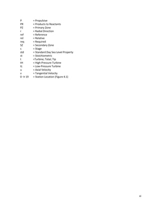
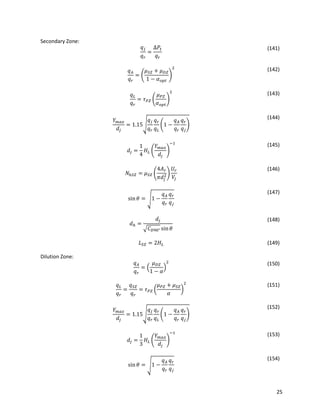
and the AEDsys design are describe in great detail. For reference, Figure 4.1 is a cross section of low
bypass turbofan engine with the station number locations.
Figure 4.1: Low Bypass Turbofan Station Numbering
4.1 Parametric Analysis
In order to compare the results of the given baseline turbojet engine to the newly developed low bypass
turbofan engine, a mathematical approach was initially considered. An analysis of a real engine required
a multitude of equations to be used. By applying the inputs of the turbojet with afterburner to a mixed-
flow low bypass turbofan with afterburner at each flight condition needed for the aircraft. Equations (1 –
45), listed below, can be used as an initial analysis for a mixed-flow low bypass turbofan with afterburner.
To simplify the process, the ONX program provided by AEDsys is used to do the parametric analysis
calculations. The results can be found in Appendix 12. After completing the analysis, a comparison
between both engines can be made. The fan pressure ratio and polytrophic efficiency of the fan were
initially assumed based on statistical data found in previous low bypass turbofan engines. Through
multiple iterations, the fan parameters can be finalized in order [2] to achieve the needed fuel
consumption and thrust.
Rc =
γc − 1
γc
cpc
(1)
Rt =
γt − 1
γt
cpt
(2)
RAB =
γAB − 1
γAB
cAB
(3)
a0 = √γcRcgcT0
(4)

22. 11
V0 = a0M0 (5)
τr = 1 +
γc − 1
2
M0
2 (6)
πr = τr
γc γc−1⁄ (7)
ηr = 1 for M0 ≤ 1 (8)
ηr = 1 − 0.075(M0 − 1)1.35
for M0 > 1 (9)
πd = πdmaxηr (10)
τλ =
cptTt4
cpcT0
(11)
τλAB =
cpABTt7
cpcT0
(12)
τc = πc
(γc−1) (γcec)⁄ (13)
τf = πf
(γc−1) (γcef)⁄ (14)
f =
τλ − τrτc
ηbhPR (cpcT0)⁄ − τλ
(15)
α =
ηm(1 + f)(τλ τr⁄ ){1 − [πf (πcπb)⁄ ](γt−1)ec γt⁄
} − (τc − 1)
τf − 1
(16)
τt = 1 −
1
ηm(1 + f)
τr
τλ
[τc − 1 + α(τf − 1)]
(17)
πt = τt
γt [(γt−1)et]⁄ (18)
𝑃𝑡16
𝑃𝑡6
=
𝜋 𝑓
𝜋 𝑐 𝜋 𝑏 𝜋 𝑡
(19)
𝑀16 = √
2
𝛾𝑐 − 1
{[
𝑃𝑡16
𝑃𝑡6
(1 +
𝛾𝑡 − 1
2
𝑀6
2
)
𝛾𝑡 (𝛾𝑡−1)⁄
]
(𝛾𝑐−1) 𝛾𝑐⁄
− 1}
(20)
𝛼′
=
𝛼
1 + 𝑓
(21)
𝑐 𝑝6𝐴 =
𝑐 𝑝𝑡 + 𝛼′
𝑐 𝑝𝑐
1 + 𝛼′
(22)

23. 12
𝑅6𝐴 =
𝑅𝑡 + 𝛼′
𝑅 𝑐
1 + 𝛼′
(23)
𝛾6𝐴 =
𝑐 𝑝6𝐴
𝑐 𝑝6𝐴 − 𝑅6𝐴
(24)
𝑇𝑡16
𝑇𝑡6
=
𝑇0 𝜏 𝑟 𝜏 𝑓
𝑇𝑡4 𝜏 𝑡
(25)
𝜏 𝑀 =
𝑐 𝑝𝑡
𝑐 𝑝6𝐴
1 + 𝛼′
(𝑐 𝑝𝑐 𝑐 𝑝𝑡)⁄ (𝑇𝑡16 𝑇𝑡6)⁄
1 + 𝛼′
(26)
𝜑(𝑀6, 𝛾6) =
𝑀6
2{1 + [(𝛾𝑡 − 1) 2⁄ ]𝑀6
2}
(1 + 𝛾𝑡 𝑀6
2
)2
(27)
𝜑(𝑀16, 𝛾16) =
𝑀16
2 {1 + [(𝛾𝑐 − 1) 2⁄ ]𝑀16
2 }
(1 + 𝛾𝑐 𝑀16
2
)2
(28)
𝛷 =
[
1 + 𝛼′
1
√𝜑(𝑀6, 𝛾6)
+ 𝛼′√
𝑅 𝑐 𝛾𝑡
𝑅𝑡 𝛾𝑐
𝑇𝑡16 𝑇𝑡6⁄
𝜑(𝑀16, 𝛾16)
]
2
𝑅6𝐴 𝛾𝑡
𝑅𝑡 𝛾6𝐴
𝜏 𝑀
(29)
𝑀6𝐴 = √
2𝛷
1 − 2𝛾6𝐴 𝛷 + √1 − 2(𝛾6𝐴 + 1)𝛷
(30)
𝐴16
𝐴6
=
𝛼′
√𝑇𝑡16 𝑇𝑡6⁄
𝑀16
𝑀6
√
𝛾𝑐 𝑅𝑡
𝛾𝑡 𝑅 𝑐
1 + [(𝛾𝑐 − 1) 2]⁄ 𝑀16
2
1 + [(𝛾𝑡 − 1) 2]⁄ 𝑀6
2
(31)
𝜋 𝑀 𝑖𝑑𝑒𝑎𝑙 =
(1 + 𝛼′
)√ 𝜏 𝑀
1 + 𝐴16 𝐴6⁄
𝑀𝐹𝑃(𝑀6, 𝛾𝑡, 𝑅𝑡)
𝑀𝐹𝑃(𝑀6𝐴, 𝛾6𝐴, 𝑅6𝐴)
(32)
𝜋 𝑀 = 𝜋 𝑀 𝑚𝑎𝑥 𝜋 𝑀 𝑖𝑑𝑒𝑎𝑙 (33)
𝑃𝑡9
𝑃9
=
𝑃0
𝑃9
𝜋 𝑟 𝜋 𝑑 𝜋 𝑐 𝜋 𝑏 𝜋 𝑡 𝜋 𝑀 𝜋 𝐴𝐵 𝜋 𝑛
(34)
Afterburner off:
𝑐 𝑝9 = 𝑐 𝑝6𝐴 𝑅9 = 𝑅6𝐴 𝛾9 = 𝛾6𝐴 𝑓𝐴𝐵 = 0

24. 13
𝑇9
𝑇0
=
𝑇𝑡4 𝜏 𝑡 𝜏 𝑀 𝑇0⁄
(𝑃𝑡9 𝑃9)⁄ (𝛾9−1) 𝛾9⁄
(35)
Afterburner on:
𝑐 𝑝9 = 𝑐 𝐴𝐵 𝑅9 = 𝑅 𝐴𝐵 𝛾9 = 𝛾 𝐴𝐵
𝑓𝐴𝐵 = (1 +
𝑓
1 + 𝛼
)
𝜏 𝜆𝐴𝐵 − (𝑐 𝑝6𝐴 𝑐 𝑝𝑡⁄ )𝜏 𝜆 𝜏 𝑡 𝜏 𝑀
𝜂 𝐴𝐵ℎ 𝑃𝑅 (𝑐 𝑝𝑐 𝑇0) − 𝜏 𝜆𝐴𝐵⁄ (36)
𝑇9
𝑇0
=
𝑇𝑡7 𝑇0⁄
(𝑃𝑡9 𝑃9)⁄ (𝛾9−1) 𝛾9⁄
(37)
Continue:
𝑀9 = √
2
𝛾9 − 1
[(
𝑃𝑡9
𝑃9
)
(𝛾9−1) 𝛾9⁄
− 1] (38)
𝑉9
𝑎0
= 𝑀9√
𝛾9 𝑅9 𝑇9
𝛾𝑐 𝑅 𝑐 𝑇0
(39)
𝑓𝑂 =
𝑓
1 + 𝛼
+ 𝑓𝐴𝐵
(40)
𝐹
𝑚̇ 0
=
𝑎0
𝑔𝑐
[(1 + 𝑓𝑂)
𝑉9
𝑎0
− 𝑀0 + (1 + 𝑓𝑂)
𝑅9
𝑅 𝑐
𝑇9 𝑇0⁄
𝑉9 𝑎0⁄
1 − 𝑃0 𝑃9⁄
𝛾𝑐
]
(41)
𝑆 =
𝑓𝑂
𝐹 𝑚̇ 0⁄
(42)
𝜂 𝑃 =
2𝑔𝑐 𝑉0(𝐹 𝑚̇ 0)⁄
𝑎0
2
[(1 + 𝑓𝑂)(𝑉9 𝑎0)⁄ 2
− 𝑀0
2
]
(43)
𝜂 𝑇 =
𝑎0
2
[(1 + 𝑓𝑂)(𝑉9 𝑎0)⁄ 2
− 𝑀0
2
]
2𝑔𝑐 𝑓𝑂ℎ 𝑃𝑅
(44)
𝜂 𝑂 = 𝜂 𝑃 𝜂 𝑇 (45)
4.2 AEDsys Software Analysis
When utilizing the AEDsys software provided, each individual stage must be calculated prior. By utilizing
the processes given by “Aircraft Engine Design” [1] book, the needed results can be found. Upon finding
these results, certain numbers can be placed in each stage of the AEDsys software. Once each stage is
filled in, the entire engine can be analyzed. The analysis will thus prove if the calculated results will provide
an engine suitable for the T-38 aircraft. Below are the given requirements and steps needed to accomplish
the task.

25. 14
4.2.1 Inlet
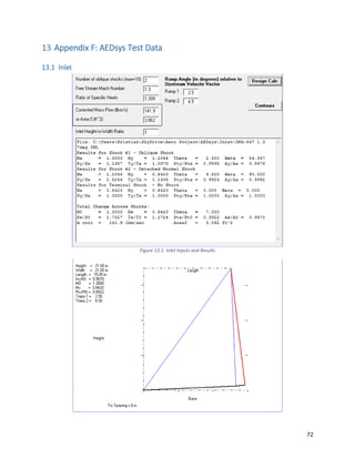
The INLET program of the AEDsys software is used to design a 2-D External Compression Inlet. Below in
Figure 4.2 an example of external compression inlet is given from Mattingly’s Aircraft Engine Design [2].
The inlet is designed for the desired maximum Mach velocity and flight condition. Before the inlet design
and calculations can be made the Inlet program asks for the following inputs: a chosen number of oblique
shocks, and their ramp angles (in degrees) relative to the Upstream Velocity Vector, the Free Stream Mach
Number, the Ratio of Specific Heats, the Corrected Mass Flow (lbm/s) or Area 0 (ft2
), and lastly the desired
Inlet Height-to-Width Ratio. Upon the completion of entering the inputs the user can press the Design
Calc button to return a sketch and dimensions of the design inlet. Additionally, the calculated performance
results across each oblique shock, an internal normal shock, and total change across the shocks is
returned.
Figure 4.2: External compression inlet
From the results a contour plot may be designed by pressing the Contours button. A window will emerge
asking the user to choose the desired x-axis and y-axis variables with the ability to select the variable
minimum and maximum values for each, the number of calculations to be made up to a max of 100, and
then a button to calculate the points for the plot contour data. Once these points are calculated the user
has a choice between having a standard black and white plot or a color plot to be made. Using the contour
plot, one can estimate the optimum values of either variable relative to the Inlet Total Pressures (Pts/Pt0)
described by the legend on the right side of the window. Refer to Appendix E for results of the INLET
program. Similarly refer to Appendix D: inlet inputs and requirements tables for Capture Area Estimations.

26. 15
The following equations, charts, and figures from the paper, “Preliminary Design of a 2D Supersonic Inlet
to Maximize Total Pressure Recover,” [3] are used as a reference to the Inlet program results:
Figure 4.3: Shock Pressure Recovery for Freestream Mach Number and Number of Oblique Shocks
Figure 4.4: Multi Shock Compression for Oswatisch Optimization
𝑀1 sin 𝜃1 = 𝑀2 sin 𝜃2 = ⋯ = 𝑀 𝑛−1 sin 𝜃 𝑛−1 (46)
Mach number and Turning Angle Calculations across each Oblique Shock (Ramp)
𝑀1
2
=
(𝛾 − 1)2
𝑀0
4
𝑠𝑖𝑛2
𝜃1 − 4(𝑀0
2
𝑠𝑖𝑛2
𝜃1 − 1)(𝛾𝑀0
2
𝑠𝑖𝑛2
𝜃1 + 1)
[2𝛾𝑀0
2
𝑠𝑖𝑛2 𝜃1 − (𝛾 + 1)][(𝛾 − 1)𝑀0
2
𝑠𝑖𝑛2 𝜃1 + 2] (47)

27. 16
tan 𝛿1 =
2𝑐𝑜𝑡𝜃1(𝑀0
2
𝑠𝑖𝑛2
𝜃1 − 1)
2 + 𝑀0
2
(𝛾 + 1 − 2𝑠𝑖𝑛2 𝜃1) (48)
𝑀2
2
=
(𝛾 − 1)2
𝑀1
4
𝑠𝑖𝑛2
𝜃2 − 4(𝑀1
2
𝑠𝑖𝑛2
𝜃2 − 1)(𝛾𝑀1
2
𝑠𝑖𝑛2
𝜃2 + 1)
[2𝛾𝑀1
2
𝑠𝑖𝑛2 𝜃2 − (𝛾 + 1)][(𝛾 − 1)𝑀1
2
𝑠𝑖𝑛2 𝜃2 + 2] (49)
tan 𝛿2 =
2𝑐𝑜𝑡𝜃2(𝑀1
2
𝑠𝑖𝑛2
𝜃2 − 1)
2 + 𝑀1
2
(𝛾 + 1 − 2𝑠𝑖𝑛2 𝜃2) (50)
Applying the optimum criteria from Eq. (4.46):
𝑀0 sin 𝜃1 = 𝑀1 sin 𝜃2 (51)
M2 is assumed to be equal to M3_up, and M3 _up will be a given input parameter, therefore M2
is known.
𝑀2 = 𝑀3_𝑢𝑝
(52)
Since M3_up is given, M3, the Mach number just after the normal shock, is calculated by the
normal shock equation:
𝑀3
2
=
(𝛾 − 1)𝑀3
2
_𝑢𝑝 + 2
2𝛾𝑀3
2
_𝑢𝑝 − (𝛾 − 1) (53)
In order to calculate M4, assume that M5 and hub-tip ratio h_t is given based on engine data.
Assuming the duct diameter is constant from 4 to 5, we have the following relation for the
airflow areas:
𝐴4
𝐴5
=
1
1 − ℎ_𝑡2 (54)
𝐴4
𝐴5
=
𝐴4
𝐴∗⁄
𝐴5
𝐴∗⁄ (55)
According to the Area-Mach number relation, we have:
(
𝐴5
𝐴∗
)
2
=
1
𝑀5
2 [
2
𝛾 − 1
(1 +
𝛾 − 1
2
𝑀5
2
)]
𝛾+1
𝛾−1
(56)
(
𝐴4
𝐴∗
)
2
=
1
𝑀4
2 [
2
𝛾 − 1
(1 +
𝛾 − 1
2
𝑀4
2
)]
𝛾+1
𝛾−1
(57)
With M5 known and using Eq. (54-58), the equation solving for M4 is derived.

28. 17
𝑀4 =
√
2
𝛾 + 1
𝛾+1
𝛾−1
(
𝐴5
𝐴∗)
2
−
2
𝛾 + 1
𝛾+1
𝛾−1
−1 (58)
For the 2 oblique shocks, the total pressure across each oblique shock is calculated as
the following:
𝑃𝑅𝑖 = [
(𝛾 + 1)𝑀𝑖−1
2
(sin 𝜃𝑖)2
(𝛾 − 1)𝑀𝑖−1
2 (sin 𝜃𝑖)2 + 2
]
𝛾
𝛾−1
[
(𝛾 + 1)
2𝛾𝑀𝑖−1
2 (sin 𝜃𝑖)2 − (𝛾 − 1)
]
1
𝛾−1
, 𝑖 = 1 − 2 (59)
The total pressure ratio across the normal shock is calculated by the following:
𝑃𝑅3 = [
(𝛾 + 1)𝑀3
2
_𝑢𝑝
(𝛾 − 1)𝑀3
2
𝑢𝑝
+ 2
]
𝛾
𝛾−1
[
(𝛾 − 1)
2𝛾𝑀3
2
𝑢𝑝
− (𝛾 − 1)
]
1
𝛾−1
(60)
From the subsonic diffuser, assume the total temperature is constant, then according to
the equation flow function, we have:
𝑃𝑅_𝑆𝑢𝑏 =
𝑃𝑡4
𝑃𝑡3
=
1
𝐴𝑅43
𝑊𝑓𝑓3
𝑊𝑓𝑓4 (61)
The flow function values Wff3 and Wff4 are determined by statics temperatures t3 and t4,
and the Mach numbers M3 and M4.
Based on Borda-Carnot loss equation, the following equation is derived with correction
factors:
𝑃𝑡4
𝑃𝑡3
= 1 − 𝐾 𝑀𝑡ℎ 𝐾𝑑 (1 −
1
𝐴𝑅43
)
2 𝛾
2 𝑀3
2
(1 +
𝛾 − 1
2 𝑀3
2
)
𝛾
𝛾−1 (62)
The coefficient KMth accounts for friction loss and Kd accounts for expansion loss. With
the values found, then the values of PR4 and AR43 are determined by solving Eq. (61) and
(62) simultaneously.
The total pressure recovery is then calculated as following:
𝑇𝑃𝑅 = ∏ 𝑃𝑅𝑖 × 𝑃𝑅_𝑠𝑢𝑏
3
𝑖=1
(63)

29. 18
Φ𝑖𝑛𝑙𝑒𝑡 =
(
𝐴0𝑖 𝑟𝑒𝑠
𝐴0 𝑟𝑒𝑞
− 1) {𝑀0 − (
2
𝛾 + 1 +
𝛾 − 1
𝛾 + 1 𝑀0
2
)
1
2
}
𝐹𝑔𝑐 (𝑚̇ 0 𝑎0)⁄
(64)
4.2.2 Fan & Compressor
One of the first steps in designing a gas turbine engine is to design the compressor. The turbine,
combustion chamber, and afterburner design are greatly determined by the outputs of the compressor.
Using the method describe in “Elements of Propulsion” [1], below is a list of the equations that were used
to calculate the initial values of each stage of the compressor. Each calculation had to be repeated for the
number of stages that were chosen for the compressor. The desired number of stages for a compressor
are determined by the designer preference, output required, and weight desired for the entire turbofan
engine. Certain inputs are initially assumed and later altered based on the designer’s preference in stage
loading, degree of reaction, stage efficiency, blade radius, blade solidity, and number of blades per stage.
These inputs include: M1, α1, α3, u2/u1, φcr, and φcs; to view typical initial guesses, see Table 11.2 located
in the Appendix D. The equations can also be used to determine the velocity triangles at each compressor
stage. The mass flow parameter can be calculated using the GASTAB program provided with the AEDSYS
software.
Air flow through an axial-flow compressor is naturally three-dimensional, which makes it extremely hard
to comprehend and analyze the flow. To simplify the design process, a two-dimensional flow field is used.
The sum of the two flow fields will give the total flow field. The two different coordinate systems are used
to describe the flow, Absolute (V = absolute velocity) is fixed to the compressor housing and the relative
(VR = relative velocity) is fixed to the rotating blades.
𝑇1 =
𝑇𝑡1
1 + (
𝛾 − 1
2 )𝑀1
2 (65)
𝑎1 = √ 𝛾𝑅𝑔𝑐 𝑇1
(66)
𝑉1 = 𝑀1 𝑎1 (67)
𝑢1 = 𝑉1 cos 𝛼1 (68)
𝜐1 = 𝑉1 sin 𝛼1 (69)
𝑃1 =
𝑃𝑡1
[1 + (
𝛾 − 1
2
) 𝑀1
2
]
𝛾
𝛾−1
(70)
MFP(M1)
𝐴1 =
𝑚̇ √ 𝑇𝑡1
𝑃𝑡1(cos 𝛼1)𝑀𝐹𝑃(𝑀1)
(71)

30. 19
𝜐1𝑅 = 𝜔𝑟 − 𝜐1 (72)
𝛽1 = tan−1
𝜐1𝑅
𝑢1
(73)
𝑉1𝑅 = √𝑢1
2
+ 𝜐1𝑅
2 (74)
𝑀1𝑅 =
𝑉1𝑅
𝑎1
(75)
𝑇𝑡1𝑅 = 𝑇1(1 +
𝛾 − 1
2
𝑀1𝑅
2
)
(76)
𝑃𝑡1𝑅 = 𝑃1(
𝑇𝑡1𝑅
𝑇1
)
𝛾
(𝛾−1) (77)
𝑃𝑡2𝑅 = 𝑃𝑡1𝑅(
𝑃𝑡2𝑅
𝑃𝑡1𝑅
)
(78)
𝑇𝑡2𝑅 = 𝑇𝑡1𝑅 (79)
𝑇𝑡2 = 𝑇𝑡1 + ∆𝑇𝑡 (80)
tan 𝛽2 =
1
1.1
[tan 𝛽2 −
𝑔𝑐 𝑐 𝑝
𝜔𝑟𝑢1
(𝑇𝑡2 − 𝑇𝑡1)
(81)
𝑢2 =
𝑢2
𝑢1
𝑢1
(82)
𝜐2𝑅 = 𝑢2 tan 𝛽2 (83)
𝑉2𝑅 = √𝑢2
2
+ 𝜐2𝑅
2 (84)
𝜐2 = 𝜔𝑟 − 𝜐2𝑅 (85)
𝛼2 = tan−1
𝜐2
𝑢2
(86)
𝑉2 = √𝑢2
2
+ 𝜐2
2 (87)
𝑇2 = 𝑇𝑡2 −
𝑉2
2
2𝑔𝑐 𝑐 𝑝
(88)
𝑃2 = 𝑃𝑡2𝑅(
𝑇2
𝑇𝑡2𝑅
)
𝛾
𝛾−1
(89)

31. 20
𝑎2 = √ 𝛾𝑅𝑔𝑐 𝑇2
(90)
𝑀2 =
𝑉2
𝑎2
(91)
𝑀2𝑅 =
𝑉2𝑅
𝑎2
(92)
𝑃𝑡2 = 𝑃2(
𝑇𝑡2
𝑇2
)
𝛾
𝛾−1 (93)
MFP(M2)
𝐴2 =
𝑚̇ √ 𝑇𝑡2
𝑃𝑡2(cos 𝛼2) 𝑀𝐹𝑃(𝑀2)
(94)
𝑇𝑡3 = 𝑇𝑡2 = 𝑇𝑡1 + ∆𝑇𝑡 (95)
𝑇3 =
𝑇𝑡3
1 + (
𝛾 − 1
2
)𝑀3
2
(96)
𝑃𝑡3 = 𝑃𝑡2(
𝑃𝑡3
𝑃3
)
(97)
𝑃3 = 𝑃𝑡3(
𝑇3
𝑇𝑡3
)
𝛾
𝛾−1
(98)
𝑎3 = √ 𝛾𝑅𝑔𝑐 𝑇3
(99)
𝑉3 = 𝑀3 𝑎3 (100)
𝑢3 = 𝑉3 cos 𝛼3 (101)
𝜐3 = 𝑉3 sin 𝛼3 (102)
𝐴3 =
𝑚̇ √ 𝑇𝑡3
𝑃𝑡3(cos 𝛼3) 𝑀𝐹𝑃(𝑀3) (103)
°𝑅 𝑐 =
𝑇2 − 𝑇1
𝑇3 − 𝑇1
(104)
𝐷𝑟 = 1 −
𝑉2𝑅
𝑉1𝑅
+
|𝜐1𝑅 − 𝜐2𝑅|
2𝜎𝑉2
(105)
𝐷𝑠 = 1 −
𝑉3
𝑉2
+
|𝜐2 − 𝜐3|
2𝜎𝑉2
(106)

32. 21
𝜂 𝑆 =
ln(𝑃𝑡3 𝑃𝑡1)⁄
𝛾−1
𝛾 − 1
(𝑇𝑡3 𝑇𝑡1) − 1⁄
(107)
𝑒 𝑐 =
𝛾 − 1
𝛾
ln(𝑃𝑡3 𝑃𝑡1)⁄
ln (𝑇𝑡3 𝑇𝑡1)⁄
(108)
𝜓 =
𝑔𝑐 𝑐 𝑝∆𝑇𝑡
(𝜔𝑟)2
(109)
Φ =
𝑢1
𝜔𝑟
(110)
After completing these calculations for each desired stage, the values can be placed in program COMPR
form the AEDsys. The COMPR program computes a more detailed analysis of each stage in the
compressor. All output data from the COMPR can be found in Appendix 13.2. Keep in mind that these
inputs will be altered to the designer’s needed specifications and include: (c/h)s, (c/h)r, σs, and σr. It is
important to know that the number of blades are typically calculated based on the tip solidity and that a
solidity of 1 should be chosen for an optimum stage. COMPR will help determine the number of blades
for the stator and rotor in each stage. The output data form COMPR was use to generate a 3 dimensional
CAD model with the help of SOLIDWORKS shown if Figure 4.5.
Figure 4.5: CAD of First Stage Low Pressure Fan Blade
4.2.3 Combustion Chamber
Once the high pressure compressor and turbine are completed, the combustion chamber (main burner)
analysis can begin. The resulting radii for the compressor final stage and turbine first stage will be needed
in order to obtain values for the combustion chamber layout. Typically, the outer radius of the turbine
first stage will be used as the outer radius of the main burner. The program MAINBRN from the AEDsys
software is used to finalize the results for the calculations made from equations (111 - 158) below. Before
starting the design method, one must take into considerations the requirements and ranges of a

33. 22
combustion chamber. To view the optimal ranges as well as the requirements, Table 11.4 can be viewed
in the Appendix.
In the design of the main burner, there are three typical diffusers that can be used in the MAINBRN
program. The three types of diffusers are: flat-wall, dump, and combined. For the combined diffuser,
typically two to three streams are used in a flat-wall that discharges into a dump. To view the operating
regimes of these three diffusers as well as the geometries, see the figures below. The diffuser is used to
slow down the air before entering the primary zone, this is to ensure complete combustion as well as
reduce the chances of flame-out. For initial design, the equations below will only take into consideration
the flat-wall. Although used for initial design, the combined diffuser typically provides better results but
the diffuser selection will be based on the designer.
Figure 4.6: Operating regimes
Figure 4.7: Geometry of flat-wall diffuser
Figure 4.8: Geometry of dump diffuser
Figure 4.9: Geometry of combined diffuser
After leaving the diffuser, the air is then mixed with fuel and ignited in the primary zone. Due to the
extreme temperatures, liner cooling will be used to maintain stability of the material in the main burner.
Upon leaving, the combusted gas will enter the secondary zone and dilution zone where the air will be

34. 23
cooled to a point that will allow the turbine to maintain stability. To begin the initial design, follow the
equations listed below.
Diffuser:
𝐴𝑅 =
𝐴3.2
𝐴3.1
(111)
𝜂 𝐷 =
𝜂 𝐷𝑚 𝐴𝑅2(1 − [𝐴3.1 𝐴 𝑚⁄ ]2) + 2(𝐴𝑅[𝐴3.1 𝐴 𝑚⁄ ] − 1)
𝐴𝑅2 − 1
(112)
(
𝛥𝑃𝑡
𝑞1
)
𝐷
= (1 −
1
𝐴𝑅2
)(1 − 𝜂 𝐷)
(113)
𝜋 𝐷 = 1 −
(∆𝑃𝑡 𝑞1⁄ ) 𝐷
1 + 2 𝛾𝑀3.1
2⁄
(114)
𝐴 𝑚 = 𝜂 𝐷𝑚(𝐴𝑅)𝐴3.1 (115)
𝐿 = 𝐻3.1 (
𝑟 𝑚3.1
𝑟 𝑚3.2
)
𝐴𝑅 − 1
2 tan 4.5𝑑𝑒𝑔
(116)
∆𝑥 = √𝐿2 − (𝑟3.1 − 𝑟3.2)2 (117)
Air Partitioning:
𝜑4 =
𝑚̇ 𝑓𝑀𝐵
𝑓𝑠𝑡 𝑚̇ 3.1
(118)
∆𝑇 𝑚𝑎𝑥 =
𝑇𝑡4 − 𝑇3.1
𝜑4
(119)
𝜑 𝑆𝑍 =
𝑇𝑔 − 𝑇3.1
∆𝑇 𝑚𝑎𝑥
(120)
𝜑 𝑃𝑍 =
𝜑 𝑆𝑍
𝜀 𝑃𝑍
(121)
𝜇 𝑃𝑍 =
𝜑4
𝜑 𝑃𝑍
(122)
𝜇 𝑆𝑍 =
𝜑4
𝜑 𝑆𝑍
−
𝜑4
𝜑 𝑃𝑍
(123)
𝑇𝑔 = 𝑇𝑡3.1 + 𝜑 𝑃𝑍 𝜀 𝑃𝑍∆𝑇 𝑚𝑎𝑥 (124)
𝛷 =
𝑇𝑔 − 𝑇 𝑚
𝑇𝑔 − 𝑇3.1
(125)

35. 24
For Film Cooling:
𝜇 𝑐 =
1
6
(
𝑇𝑔 − 𝑇 𝑚
𝑇 𝑚 − 𝑇3.1
)
(126)
For Transpiration or Effusion Cooling:
𝜇 𝑐 =
1
25
(
𝑇𝑔 − 𝑇 𝑚
𝑇 𝑚 − 𝑇3.1
)
(127)
𝜇 𝐷𝑍 = 1 − (𝜇 𝑃𝑍 + 𝜇 𝑆𝑍 + 𝜇 𝑐) (128)
Dome and Liner:
(
∆𝑃𝑡
𝑞 𝑟
)
𝑀𝐵
=
𝑃𝑡3.2 − 𝑃𝑡4
𝑃𝑡3.2 − 𝑃3.2
(129)
𝑚̇ 𝐴
𝑚̇ 𝑟
= 𝜇 𝑆𝑍 + 𝜇 𝐷𝑍
(130)
𝛼 𝑜𝑝𝑡 = 1 − (
𝑚̇ 𝐴
𝑚̇ 𝑟
)
2 3⁄
(
∆𝑃𝑡
𝑞 𝑟
)
𝑀𝐵
−1 3⁄ (131)
𝐻𝐿 = 𝛼 𝑜𝑝𝑡 𝐻𝑟 (132)
Total Pressure Loss:
𝜏 𝑃𝑍 =
𝑇𝑔
𝑇𝑡3.2
(133)
(
∆𝑃𝑡
𝑞 𝑟
)
𝑚𝑖𝑛
= (
𝜇 𝑃𝑍
𝛼 𝑜𝑝𝑡
)
2
𝜏 𝑃𝑍(2𝜏 𝑃𝑍 − 1)
(134)
Primary Zone:
𝑉𝑗 = 𝑈𝑟√(
∆𝑃𝑡
𝑞 𝑟
)
𝑀𝐵
(135)
𝐶 𝐷90° = {
0.64 𝑓𝑜𝑟 𝑝𝑙𝑎𝑖𝑛 ℎ𝑜𝑙𝑒𝑠
0.81 𝑓𝑜𝑟 𝑝𝑙𝑢𝑛𝑔𝑒𝑑 ℎ𝑜𝑙𝑒𝑠
(136)
𝑟𝑡 = √ 𝑟ℎ
2
+
𝑚̇ 𝑃𝑍 − 3𝑚̇ 𝑓𝑀𝐵
𝑁𝑛𝑜𝑧 𝜋𝐶 𝐷90° cos 𝛼 𝑠𝑤
(
𝐴 𝑟
𝑚̇ 𝑟
) (
∆𝑃𝑡
𝑞 𝑟
)
𝑀𝐵
−1 2⁄ (137)
𝑆′
=
2
3
tan 𝛼 𝑠𝑤 [
1 − (𝑟ℎ 𝑟𝑡⁄ )3
1 − (𝑟ℎ 𝑟𝑡⁄ )2
]
(138)
𝐴 𝑆𝑊 = 𝜋(𝑟𝑡
2
− 𝑟ℎ
2
) (139)
𝐿 𝑃𝑍 = 2𝑆′
𝑟𝑡 (140)

36. 25
Secondary Zone:
𝑞 𝑗
𝑞 𝑟
=
∆𝑃𝑡
𝑞 𝑟
(141)
𝑞 𝐴
𝑞 𝑟
= (
𝜇 𝑆𝑍 + 𝜇 𝐷𝑍
1 − 𝛼 𝑜𝑝𝑡
)
2 (142)
𝑞 𝐿
𝑞 𝑟
= 𝜏 𝑃𝑍 (
𝜇 𝑃𝑍
𝛼 𝑜𝑝𝑡
)
2 (143)
𝑌 𝑚𝑎𝑥
𝑑𝑗
= 1.15√
𝑞𝑗
𝑞 𝑟
𝑞 𝑟
𝑞 𝐿
(1 −
𝑞 𝐴
𝑞 𝑟
𝑞 𝑟
𝑞 𝑗
)
(144)
𝑑𝑗 =
1
4
𝐻𝐿 (
𝑌 𝑚𝑎𝑥
𝑑𝑗
)
−1 (145)
𝑁ℎ𝑆𝑍 = 𝜇 𝑆𝑍 (
4𝐴 𝑟
𝜋𝑑𝑗
2)
𝑈𝑟
𝑉𝑗
(146)
sin 𝜃 = √1 −
𝑞 𝐴
𝑞 𝑟
𝑞 𝑟
𝑞 𝑗
(147)
𝑑ℎ =
𝑑𝑗
√𝐶 𝐷90° sin 𝜃
(148)
𝐿 𝑆𝑍 = 2𝐻𝐿 (149)
Dilution Zone:
𝑞 𝐴
𝑞 𝑟
= (
𝜇 𝐷𝑍
1 − 𝛼
)
2 (150)
𝑞 𝐿
𝑞 𝑟
=
𝑞 𝑆𝑍
𝑞 𝑟
= 𝜏 𝑃𝑍 (
𝜇 𝑃𝑍 + 𝜇 𝑆𝑍
𝛼
)
2 (151)
𝑌 𝑚𝑎𝑥
𝑑𝑗
= 1.15√
𝑞𝑗
𝑞 𝑟
𝑞 𝑟
𝑞 𝐿
(1 −
𝑞 𝐴
𝑞 𝑟
𝑞 𝑟
𝑞 𝑗
)
(152)
𝑑𝑗 =
1
3
𝐻𝐿 (
𝑌 𝑚𝑎𝑥
𝑑𝑗
)
−1 (153)
sin 𝜃 = √1 −
𝑞 𝐴
𝑞 𝑟
𝑞 𝑟
𝑞 𝑗
(154)

37. 26
𝑑ℎ =
𝑑𝑗
√𝐶 𝐷90° sin 𝜃
(155)
𝑁ℎ𝐷𝑍 = 𝜇 𝐷𝑍 (
4𝐴 𝑟
𝜋𝑑𝑗
2)
𝑈𝑟
𝑉𝑗
(156)
𝐿 𝐷𝑍 = 1.5𝐻𝐿 (157)
Total Length:
𝐿 𝐿 = 𝐿 𝑃𝑍 + 𝐿 𝑆𝑍 + 𝐿 𝐷𝑍 (158)
4.2.4 Turbine
Upon completing the initial calculations for the compressor, the turbine calculations can be started. Based
on the number of high pressure and low pressure stages of both the fan and compressor will determine
the number of stages in the turbine. The high pressure turbine(s) will power the high pressure compressor
stages, the low pressure turbine(s) will power both the low pressure compressor and fan stages. The
decision on the number of stages for both high and low pressure turbines will be based upon weight,
designer preference, stage loading, and power needed to drive the compressor. Once the designer
achieves desired results, the turbine calculations will be completed. Below is a list of equations (159 - 192)
for calculating the mean-radius stage for stator and rotor flow with losses. The equations can also be used
to determine the velocity triangles at each turbine stage. Certain inputs are initially assumed and later
altered based on the designer’s preference in stage loading, degree of reaction, stage efficiency, blade
radius, blade solidity, and number of blades per stage. These inputs include: M2, α1, α3, u3/u2, φt stator, and
φt rotor; to view typical initial guesses, see Table 11.5 located in the Appendix. It is important to keep in
mind that M2 must be supersonic at the first turbine stage in order to obtained choked flow but should
not cause M3 to be greater than 0.9. It is also important to note that a desirable multistage design would
have the total temperature difference distributed evenly among each stage. Within each stage, the total
temperature at station two will equal that of station one (i.e. Tt1 = Tt2). It can also be seen that the stage
loading should remain between 1.4 and 2 for modern aircraft engines. For simplicity of design, α1 will
remain the same throughout each stage of the turbine.
𝑇1 =
𝑇𝑡1
1 + [(𝛾 − 1)/2]𝑀1
2
(159)
𝑉1 = √
2𝑔𝑐 𝑐 𝑝 𝑇𝑡1
1 + 2 [(𝛾 − 1)𝑀1
2]⁄
(160)
𝑢1 = 𝑉1 cos 𝛼1 (161)
𝑣1 = 𝑉1 sin 𝛼1 (162)
𝑇2 =
𝑇𝑡2
1 + [(𝛾 − 1) 2⁄ ]𝑀2
2
(163)

38. 27
𝑉2 = √
2𝑔𝑐 𝑐 𝑝 𝑇𝑡2
1 + 2 [(𝛾 − 1)𝑀2
2]⁄
(164)
𝜓 =
𝑔𝑐 𝑐 𝑝(𝑇𝑡1 − 𝑇𝑡3)
(𝜔𝑟)2
(165)
𝛼2 = sin−1
(𝜓
𝜔𝑟
𝑉2
) − (
𝑢3
𝑢2
tan 𝛼3) √1 + (
𝑢3
𝑢2
tan 𝛼3)
2
− (𝜓
𝜔𝑟
𝑉2
)
2
1 + (
𝑢3
𝑢2
tan 𝛼3)
2
(166)
𝑢2 = 𝑉2 cos 𝛼2 (167)
𝑣2 = 𝑉2 sin 𝛼2 (168)
𝛷 =
𝑢2
𝜔𝑟
(169)
𝑉3 =
𝑢3
𝑢2
cos 𝛼2
cos 𝛼3
(170)
𝑢3 = 𝑉3 cos 𝛼3 (171)
𝑣3 = 𝑉3 sin 𝛼3 (172)
°𝑅𝑡 = 1 −
1
2𝜓
(
𝑉2
𝜔𝑟
)
2
[1 − (
𝑢3 cos 𝛼2
𝑢2 cos 𝛼3
)
2
]
(173)
𝑇3 = 𝑇2 − °𝑅𝑡(𝑇𝑡1 − 𝑇𝑡3) (174)
𝑀3 = 𝑀2
𝑉3
𝑉2
√
𝑇2
𝑇3
(175)
𝑀2𝑅 = 𝑀2√cos2 𝛼2 + (sin 𝛼2 −
𝜔𝑟
𝑉2
)
2
(176)
𝑀3𝑅 = 𝑀3√cos2 𝛼3 + (sin 𝛼3 −
𝜔𝑟
𝑉3
)
2
(177)
𝑇𝑡3𝑅 = 𝑇𝑡2𝑅 = 𝑇𝑡3 +
𝑉3
2
2𝑔𝑐 𝑐 𝑝
[cos2
𝛼3 + (sin 𝛼3 +
𝜔𝑟
𝑉3
)
2
− 1]
(178)

39. 28
𝜏 𝑠 =
𝑇𝑡3
𝑇𝑡1
(179)
𝑍𝑠 𝑐 𝑥
𝑠
= (2 cos2
𝛼2) (tan 𝛼1 +
𝑢2
𝑢1
tan 𝛼2) (
𝑢1
𝑢2
)
2 (180)
𝛽2 = tan−1
𝑣2 − 𝜔𝑟
𝑢2
(181)
𝛽3 = tan−1
𝑣3 + 𝜔𝑟
𝑢3
(182)
𝑍 𝑟 𝑐 𝑥
𝑠
= (2 cos2
𝛽3) (tan 𝛽2 +
𝑢3
𝑢2
tan 𝛽3)(
𝑢2
𝑢3
)
2 (183)
𝑃1 = 𝑃𝑡1 (
𝑇1
𝑇𝑡1
)
𝛾 (𝛾−1)⁄ (184)
𝑃𝑡2 =
𝑃𝑡1
1 + 𝜑 𝑡 𝑠𝑡𝑎𝑡𝑜𝑟[1 − (𝑇2 𝑇𝑡2⁄ ) 𝛾 (𝛾−1)⁄ ]
(185)
𝑃2 = 𝑃𝑡2 (
𝑇2
𝑇𝑡2
)
𝛾 (𝛾−1)⁄ (186)
𝑃𝑡2𝑅 = 𝑃2 (
𝑇𝑡2𝑅
𝑇2
)
𝛾 (𝛾−1)⁄ (187)
𝑃𝑡3𝑅 =
𝑃𝑡2𝑅
1 + 𝜑 𝑡 𝑟𝑜𝑡𝑜𝑟[1 − (𝑇3 𝑇𝑡3𝑅⁄ ) 𝛾 (𝛾−1)⁄ ]
d
(188)
𝑃3 = 𝑃𝑡3𝑅 (
𝑇3
𝑇𝑡3𝑅
)
𝛾 (𝛾−1)⁄ (189)
𝑃𝑡3 = 𝑃3 (
𝑇𝑡3
𝑇3
)
𝛾 (𝛾−1)⁄ (190)
𝜋 𝑠 =
𝑃𝑡3
𝑃𝑡1
(191)
𝜂 𝑠 =
1 − 𝜏 𝑠
1 − 𝜋 𝑠
(𝛾−1) 𝛾⁄
(192)
After completing the calculations for each desired stage; the flow annulus area, radii, and number of
blades can be calculated for each stator and rotor. Below is a list of equations (193 - 211) that allow for
completion of the calculation process. Upon completing the calculations, the values found can be placed

40. 29
in the AEDSYS software using the TURBN program. Before beginning the calculations, it should be known
that the Zweifel coefficient shall remain close to 1 for an optimum stage. Along with this, the chord/height
ratio shall remain between 0.3 and 1. As stated before, initial inputs will be assumed and typical assumed
inputs can be seen in the Appendix. These inputs will be altered to the designer’s needed specifications
and include: (c/h)s, (c/h)r, Zs, Zr, σs, and σr. The assumed solidities will be made for the hub, mean, and tip
of the blades. It is important to know that the number of blades are typically calculated based on the tip
solidity. The mass flow parameter can be calculated using the GASTAB program provided with the AEDSYS
software.
Station 1 and 2R:
𝐴1 =
𝑚̇ √ 𝑇𝑡1
𝑃𝑡1 𝑀𝐹𝑃(𝑀1)(cos 𝛼1)
(193)
ℎ1 =
𝐴1
2𝜋𝑟 𝑚
= 𝑟𝑡1 − 𝑟ℎ1
(194)
𝑣1ℎ = 𝑣1𝑚 = 𝑣1𝑡 = 0 (195)
Station 2 and 3R:
𝐴2 =
𝑚̇ √ 𝑇𝑡2
𝑃𝑡2 𝑀𝐹𝑃(𝑀2)(cos 𝛼2)
(196)
ℎ2 =
𝐴2
2𝜋𝑟 𝑚
= 𝑟𝑡2 − 𝑟ℎ2
(197)
𝑣2ℎ = 𝑣2𝑚
𝑟 𝑚
𝑟2ℎ
(198)
𝛼2ℎ = tan−1
𝑣2ℎ
𝑢2
(199)
𝑣2𝑡 = 𝑣2𝑚
𝑟 𝑚
𝑟2𝑡
(200)
𝛼2𝑡 = tan−1
𝑣2𝑡
𝑢2
(201)
𝑐 =
𝑐
ℎ
ℎ1 + ℎ2
2
(202)
𝑍𝑠,𝑟 (
𝑐 𝑥
𝑠
)
𝑚,ℎ,𝑡
= (2 cos2
𝛼2𝑚,2ℎ,2𝑡)(tan 𝛼2𝑚,2ℎ,2𝑡 +
𝑢2
𝑢1
tan 𝛼2𝑚,2ℎ,2𝑡)(
𝑢1
𝑢2
)
2 (203)
(
𝑐 𝑥
𝑠
)
𝑚,ℎ,𝑡
=
𝑍𝑠,𝑟 (
𝑐 𝑥
𝑠 )
𝑚,ℎ,𝑡
𝑍𝑠,𝑟
(204)
𝛾1𝑚,1ℎ,1𝑡 = 𝛼1𝑚,1ℎ,1𝑡 = 0 (205)

41. 30
𝛾2𝑚,2ℎ,2𝑡 =
𝛾1𝑚,1ℎ,1𝑡 + 8√ 𝜎 𝑚,ℎ,𝑡 𝛼2𝑚,2ℎ,2𝑡
8√ 𝜎 𝑚,ℎ,𝑡 − 1
(206)
𝜃2𝑚,2ℎ,2𝑡 =
𝛾2𝑚,2ℎ,2𝑡 − 𝛾1𝑚,1ℎ,1𝑡
2
(207)
𝜎 𝑚,ℎ,𝑡 =
(𝑐 𝑥 𝑠⁄ ) 𝑚,ℎ,𝑡
cos 𝜃 𝑚,ℎ,𝑡
(208)
𝑠 𝑚,ℎ,𝑡 =
𝜎 𝑚,ℎ,𝑡
𝑐
(209)
𝑐 𝑥 = 𝑠 𝑚,ℎ,𝑡 𝜎 𝑚,ℎ,𝑡 cos 𝜃2𝑚,2ℎ,2𝑡 (210)
𝑁𝑏 = 2 (
𝜋𝑟2𝑚,2ℎ,2𝑡 𝜎 𝑚,ℎ,𝑡
𝑐
) (211)
As seen above, equations (193 - 211) can be used to find the number of blades for the mean, hub, and tip
of each station in the turbine. Typically, if the number of blades is any decimal then it will be rounded up
to the nearest whole number. This will be the total number of blades for each station of each turbine
stage. The values obtained can now be placed in the TURBN program.
Once the values were found for the turbine section, a computer aided drawing was made to represent
the first stage rotor blade. The model, using SOLIDWORKS, can be viewed below in Figure 4.10 to obtain
an idea of what will be expected in the final design process. It can be seen that the turbine blade is much
smaller than the compressor blades. The reason for this is that the turbine blades are more numerous for
both stator and rotor to obtain the needed power. Due to the relatively weaker programming power of
the student edition of SOLIDWORKS and insufficient time, the cooling qualities of the CAD model were
not added. Figure 4.11 can be seen below the CAD model to obtain an understanding of the cooling used
in the turbine.
Figure 4.10: CAD of the High Pressure Turbine Blade

42. 31
Figure 4.11: Turbine Transpiration and Full-Coverage Film Cooling
4.2.5 Afterburner
After the main turbofan engine components have been completed, the design of the afterburner can
begin. The output data of the TURBN and the ONX programs can be used for the input data to the
AFTRBRN program. The design of an afterburner generally follows the design of the combustion chamber.
The following inputs are need for the AFTRBRN program: total pressure, total temperature, Mach number,
gas flow, and outer radius. It is important to note, that the outer radius of the afterburner typical does
not exceed the maximum outer radius of the engine. The geometry of the afterburner can be seen in
Figure 4.12. The afterburner fuel flow at station 6.1 can be found with the ONX program, as well as the
total pressure and temperature a station 7. A crucial design aspect of the afterburner is the time at
blowout (tBO). The tBO must be obtained from the AEDsys software program KINTEX. The follow
requirements for KINTEX are the pressure, temperature, composition of the approach gas stream, and
afterburner fuel flow rate. Once all of the pervious information is enter into TURBN, the number of spray
/ vee-gutter rings can be determined. The position of the spray / vee-gutter rings can be seen in Figure
4.13 and Figure 4.14. To make sure that the afterburner functions properly, the number of spray / vee-
gutter rings should be less than 15. To meet the desired performance, 10 spray / vee-gutter rings were
chosen. Figure 13.46 shows the layout of the completed afterburner.

43. 32
Figure 4.12: Geometry of Afterburner Figure 4.13: Flow Patterns in the Afterburner
Figure 4.14: Principal Features
4.2.6 Nozzle
The NOZZLE program from the AEDsys software is used for designing a One-Dimension/Two-Dimensional
Circular Convergent-Divergent Nozzle. Due to customer requirements and a more accurate representation
of a real nozzle, only a two-dimensional convergent-divergent nozzle was designed for the project. Initially
the inputs required by the program are as follows: mass flow rate, total pressure at station 8, total
temperature at station 8, ration of specific heats, gas constant, static pressure at station 0 or freestream,
the area ratio of area at 9 divided by the area at 8 (A9/A8), the convergent angle (degrees), the divergent
angle (degrees), and the diameter at station 7 (inches). The values can be found from the results via ONX
and AED Engine Cycle Deck Component Interfaces at each flight condition. The only disclaimer is when
using the results from the component interfaces; stages 7, 8, and 9 are considered wet. In order to
compensate for the entrance of the nozzle, conditional values are assumed when the engine is dry.
Additionally, nozzle’s convergent-divergent angles are optimized for maximum amount gross thrust actual
with the diameter at 7 being constant. Once the inputs are entered, the design results can be calculated.
A color contour plot of Divergent Angle vs A9/A8, a sketch of the nozzle’s dimensions, and performance
values are returned. The contour plot shows the optimal divergent angle relative to gross thrust constant,
Cfg. Below in Figure (4.15) and Equations (212 - 224) are used by the NOZZLE program for the output
calculations. For examples of the inputs into the program and the results produced, refer to Appendix E:
Test Data. A general guide to the values for which the CD Max, the CV, and the CA of the nozzle configurations
can be seen in Figures 11.2, 11.3, and 11.4 of Appendix D.

44. 33
Figure 4.15: Nozzle geometric parameters
𝐶𝑓𝑔 =̇ 𝐹𝑔 𝑎𝑐𝑡𝑢𝑎𝑙 𝐹𝑔 𝑖𝑑𝑒𝑎𝑙⁄ (212)
𝐶 𝐷 =̇ 𝑚̇ 8 𝑚̇ 8𝑖⁄ (213)
𝐶 𝐷 =
𝑚̇ 8
𝑚̇ 8𝑖
=
𝜌8 𝑉8 𝐴8
𝜌8 𝑉8 𝐴8𝑒
=
𝐴8
𝐴8𝑒
=
𝑃𝑡8
𝑃𝑡7
(214)
𝐶 𝑉 =̇ 𝑉9 𝑉9𝑖⁄ (215)
𝐶𝐴 =̇
1
𝑚̇
∫ cos 𝛼𝑗 𝑑𝑚̇
(216)
𝐶𝑓𝑔 𝑝𝑒𝑎𝑘 = 𝐶 𝑉 𝐶𝐴 (217)
𝐴
𝐴∗|
9𝑖
=
𝐴9
𝐶 𝐷 𝐴8
(218)
𝑉9𝑖 = √ 𝑅 𝑔 𝑐
𝑇𝑡8√
2𝛾
𝛾 − 1
{1 − (
𝑃9𝑖
𝑃𝑡9𝑖
)
(𝛾−1) 𝛾⁄
} (219)

45. 34
𝐶𝑓𝑔 =
𝐶𝑓𝑔 𝑝𝑒𝑎𝑘 𝑚̇ 7 𝑉9𝑖 𝑔𝑐⁄ + (𝑃9𝑖 − 𝑃0)𝐴9
𝑚̇ 7 𝑉𝑠 𝑔𝑐⁄
(220)
𝐹𝑔 = 𝐶𝑓𝑔 𝑝𝑒𝑎𝑘 𝑚̇ 7 𝑉9𝑖 𝑔𝑐⁄ + (𝑃9𝑖 − 𝑃0)𝐴9 (221)
𝐶 𝑉 =
𝑉9
𝑉9𝑖
= √
1 − (𝑃9 𝑃𝑡9⁄ )(𝛾−1) 𝛾⁄
1 − (𝑃9𝑖 𝑃𝑡8⁄ )(𝛾−1) 𝛾⁄
(222)
𝑃9
𝑃𝑡9
= {1 − 𝐶 𝑉
2
[1 − (
𝑃9𝑖
𝑃𝑡8
)
(𝛾−1) 𝛾⁄
]}
𝛾 (𝛾−1)⁄
(223)
𝜋 𝑛 =
𝑃𝑡9
𝑃𝑡8
= 𝐶 𝐷
𝐴 𝐴∗⁄ |9
𝐴9 𝐴8⁄
(224)
4.3 Weight Calculation Method
Due to the fact that the DKA-867 is in the preliminary stage of design, a preliminary weight estimation
was made for both the engine with and without a tailpipe. For a more in depth look as to what the exact
weight of the engine will be based on dimensioning and material choice, a CAD model will need to be
made. The CAD model will allow for a material selection for each individualized component of the engine.
Once labeled and completed, the weight of each component may be found. Although, a CAD model will
only give a valid comparison to an actual low-bypass turbofan engine. The only way to truly know the
actual weight of the engine is to create a prototype model that uses equivalent density materials or the
same materials stated below in the materials section of this report. For the case of the DKA-867, the
preliminary weight calculation can be made via equation (225) found below. This will be used to find the
weight of the engine with the afterburning section. To find the weight without afterburner, comparisons
of afterburners with similar dimensions of the one used in the DKA-867 low-bypass turbofan with
afterburner were used. Using an average of the afterburner weights found, the weight was then
subtracted from the weight found using the equation below. It can be seen that both the thrust and Mach
number used in the equation are the maximum allotted by the engine.
𝑊 = 0.063𝑇1.1
𝑀0.25
𝑒(−0.81 𝐵𝑃𝑅) (225)
4.4 Mission Analysis
The analysis of each mission needed for the Northrop Grumman T-38 Talon was determined using the
AEDsys software provided by “Aircraft Engine Design Second Edition” [2]. Upon completing the ONX
parametric analysis provided, a document will be saved with the results. Using these results, a mission
analysis can be done. To begin the analysis, the completed parametric analysis must be uploaded to the
AEDsys main program software. Once uploaded, the aircraft and engine type must be chosen based on
the needs of the designer. This will allow for a more realistic output when selecting the needed mission.
These can be selected by going to the ‘Aircraft Drag’ and ‘Engine’ tabs found on the task bar. To state how
many engines will be used in flight, the ‘Cycle Deck’ button can be opened under the ‘Engine’ tab. Next,
the ‘Mission’ button should be clicked, which will open a second screen that is used to determine a given
operation.

46. 35
Initially, the box displaying the aircraft performance and sizing can be filled out. This will allow for the
engine test to be run with the aircraft for which it is designed for. The thrust found from the NOZZLE
program output, wing area, and design takeoff weight will be filled in to update the aircraft model. Once
filled in, the ‘Empty Weight Model’ button can be pressed to estimate the empty weight of the aircraft.
Along with the atmospheric conditions updated, the mission choice can now be created.
The ‘Number of Mission Legs’ box will now be filled in to complete the inputs before the program can be
ran. Certain legs can either be added or subtracted from the box in order to determine the overall mission
required. For each leg created, an altered name can be used to display a more in depth understanding.
Within each leg of the mission, certain aspects can be altered. A few examples of these are: Mach number,
altitude, temperature, time, and distance. It is important to keep in mind exactly what the purpose of the
aircraft is used for when determining the mission legs needed. For the case of the T-38 Talon; a subsonic
cruise, supersonic burst, and loiter are a few of the key components used in the analysis. To view the
mission legs and results found for the T-38 using the DKA-867 low-bypass turbofan engine with
afterburner at each leg, Appendix 13 can be viewed.
Once the input data is filled in, the ‘Calculate’ button can be clicked to view the results. Each leg will then
provide a list of results ranging from thrust output to TSFC. These results can also be viewed by clicking
‘Summary’ upon the completion of the calculations. The summary data provided gives a brief overview of
each segment previously mentioned. Although not entirely accurate, the mission analysis of the AEDsys
main program will provide for an acceptable preliminary design. It can be seen that the landing weight of
the aircraft must be slightly larger than the empty weight calculated previously in order to prove the
validity of the results.
4.5 Results
Once the calculations were completed for each station and the mission requirements, the results had to
be studied. It can be seen in the tables below that each individual requirement set forth by AIAA was met.
By obtaining these results, it can be seen that the DKA-867 will be an excellent replacement for the J85-
GE-5A engine in current use.

47. 36
4.5.1 Compliance Matrix
Table 4.1: Compliance Matrix
General characteristics
Wing area (ft2
) 170
Max. take-off weight (lbm) 12000
Takeoff-Thrust (lbf) 8014
Design Afterburning Thrust (lbf) 3446
Performance
Maximum speed Mach 1.3
Cruise speed Mach 0.85
Mission Fuel Burn (lbs) 3488
Cruise TSFC (lbm/h/lbf) 1.002
Takeoff TSFC (lbm/hr/lbf) 1.673
Engine Weight w/o tailpipe (lbs) 407.07
Engine Weight w/ tailpipe (lbs) 517.07
Engine Length w/o tailpipe (in.) 49.12
Engine Length w/ tailpipe (in.) 102.02
Fan Diameter (in.) 20

48. 37
4.5.2 Engine Summary Data
Table 4.2: Engine Summary Data
Summary Data
Design MN 0.85
Design Altitude (ft) 35000
Design Fan Mass Flow (lbm/s) 51
Design Gross Thrust (lbf) 2050
Design Bypass Ratio 0.22
Design Net Thrust (lbf) 1597
Design Afterburning Net Thrust (lbf) 3446
Design TSFC (lbm/h/lbf) 1.002
Design Overall Pressure Ratio 6.947
Design T4.1 (R) 2000
Design Engine Pressure Ratio 2.232
Design Fan / LPC Pressure Ratio 1.850
Design Chargeable Cooling Flow #1 5%
Design Chargeable Cooling Flow #2 5%
Design Adiabatic Efficiency for HP Turbine 0.9058
Design Adiabatic Efficiency for LP Turbine 0.9123
Design Polytropic Efficiency for Fan/LP Compressor 0.89
Design Polytropic Efficiency for HP Compressor 0.90
Design HP Shaft RPM 18,812
Design LP Shaft RPM 11,077
Table 4.3: Fan / LP Compressor Flow Station Data
Flow Station Data
IGV
Fan / LP Compressor
Bypass
Stage 1 Stage 2 Stage 3
Inflow (lbm/s) 51 51 51 51 9.20
Corrected
Inflow (lbm/s)
49.40 49.40 49.40 49.40 5.31
Inflow
Total Pressure (psi)
14.70 14.70 18.33 22.49 27.22
Inflow
Total Temperature (R)
486.70 486.70 522.00 542.20 592.60
Inflow Fuel-air-Ratio N/A N/A N/A N/A N/A
Inflow Mach # 0.5 0.4 0.386 0.373 0.343
Inflow Area (in^2) 314.16 269.93 230.90 199.96 58.89
Pressure Loss/Rise
Across Component
1 1.247 1.227 1.210 1

49. 38
Table 4.4: HP Compressor Flow Station Data
IGV
HP Compressor Combustion
ChamberStage 1 Stage 2 Stage 3 Stage 4 Stage 5
Inflow (lbm/s) 41.80 41.80 41.80 41.80 41.80 41.80 36.48
Corrected
Inflow (lbm/s)
24.12 24.12 24.12 24.12 24.12 24.12 28.28
Inflow
Total Pressure (psi)
27.22 27.22 37.32 49.62 64.44 82 102.5
Inflow
Total Temperature (R)
592.60 592.6 654.2 715.9 777.5 839.1 900.8
Inflow Fuel-air-Ratio N/A N/A N/A N/A N/A N/A 0.0355
Inflow Mach # 0.35 0.5 0.475 0.453 0.434 0.417 0.386
Inflow Area (in^2) 130.07 133.66 106.38 86.69 71.92 60.58 25.595
Pressure Loss/Rise
Across Component
1 1.371 1.330 1.299 1.272 1.250 0.930
Table 4.5: Turbine & Nozzle Flow Data
HP Turbine LP Turbine EGV Afterburner Nozzle
Inflow (lbm/s) 40.62 42.71 42.71 50.89 53.13
Corrected Inflow (lbm/s) 12.11 26.62 36.58 34.409 49.040
Inflow Total Pressure (psi) 94.97 42.83 30.37 32.8 31.522
Inflow Total Temperature (R) 1924 1711 1625.5 1492 2500
Inflow Fuel-air-Ratio N/A N/A N/A 0.0236 N/A
Inflow Mach # 0.4 0.474 0.4546 0.416 0.324
Inflow Area (in^2) 60.28 115.81 165.39 177.12 307.872
Pressure Loss/Rise
Across Component
0.451 0.709 0.998 0.998 0.999
Table 4.6: Additional Information
Additional Information
Design HP Shaft Off-take Power (hp) 5016.859
Design LP Shaft Off-take Power (hp) 2105.101
Design Customer Bleed Flow 1%

50. 39
4.5.3 Required Detailed Stage and Component Information
Table 4.7: Fan / Low Pressure Compressor Detailed Data
Compressor
Fan / Low Pressure
Stage 1 Stage 2 Stage 3
Rotor Stator Rotor Stator Rotor Stator
Lieblein Diffusion Factor 0.3865 0.4851 0.3892 0.4819 0.4103 0.4900
De Haller Number 0.669 0.652 0.674 0.672 0.6632 0.6825
Stage Loading 0.4799 0.4115 0.3782
Flow Coefficient 0.5432 0.503 0.4822
Hub-to-Tip Ratio 0.375 0.4329 0.5000 0.5385 0.5806 0.6012
Number of Blades 19 22 25 28 31 33
Solidity 1.1 1.1 1.1
Pitch (in.) 2.436 2.125 1.9427 1.7709 1.6300 1.5245
Chord (in.) 2.680 2.388 2.137 1.948 1.793 1.677
Aspect Ratio 3.571 N/A 2.538 N/A 2.4320 N/A
Taper Ratio 0.9999 0.9999 0.9999
Tip Speed (rad/s) 1160
Stagger Angle (deg) N/A 34.485 N/A 41.160 N/A 44.495
Blade metal angles (deg) 50.57 18.40 53.73 28.59 55.38 33.61
Degree of Reaction 0.7328 0.7098 0.6866
Mach Numbers 0.4 0.604 0.386 0.565 0.373 0.538

51. 40
Table 4.8: High Pressure Compressor Detailed Data
Compressor
High Pressure
Stage 1 Stage 2 Stage 3 Stage 4 Stage 5
Rotor Stator Rotor Stator Rotor Stator Rotor Stator Rotor Stator
Lieblein Diffusion
Factor
0.3982 0.4818 0.4311 0.4954 0.4335 4936 0.4345 0.4914 0.4483 0.4947
De Haller Number 0.6554 0.6671 0.6768 0.6828 0.6789 0.6841 0.6837 0.6870 0.6891 0.6899
Stage Loading 0.3444 0.3019 0.2986 0.2914 0.2838
Flow Coefficient 0.3957 0.3705 0.3684 0.3640 0.3592
Hub-to-Tip Ratio 0.5788 0.6284 0.6863 0.7105 0.7397 0.7613 0.7831 0.8008 0.8280 0.8303
Number of Blades 26 31 36 40 45 50 55 61 66 72
Solidity 1.000 1.000 1.000 1.000 1.000
Pitch (in.) 1.585 1.371 1.199 1.080 0.973 0.881 0.800 0.729 0.688 0.618
Chord (in.) 1.585 1.371 1.199 1.080 0.973 0.881 0.800 0.729 0.688 0.618
Aspect Ratio 2.9823 N/A 2.5353 N/A 2.3333 N/A 2.0120 N/A 1.8289 N/A
Taper Ratio 1.000 1.000 1.000 1.000 1.000
Tip Speed (rad/s) 1970
Stagger Angle (deg) N/A 44.84 N/A 50.335 N/A 50.765 N/A 51.675 N/A 52.625
Blade metal angles
(deg)
56.66 33.02 59.42 41.25 59.64 41.89 60.12 43.23 60.63 44.62
Degree of Reaction 0.6597 0.6211 0.6052 0.5936 0.5785
Mach Numbers 0.500 0.732 0.475 0.680 0.453 0.648 0.434 0.619 0.417 0.593
Table 4.9: Turbine Detailed Data
Turbine
High Pressure Low Pressure
Stator Rotor Stator Rotor
Zweifel Coefficient 1.00 1.00 0.65 1.50
Taper Ratio 0.999 0.999
Stage Work 1.993 2.304
Stage Pressure Ratio 0.451 0.709
Degree of Reaction 0.383 0.305
Aspect Ratio N/A 2.495 N/A 3.333
AN^2 (in2
-rpm2
) 4.124 x 1010
1.844 x 1010
Number of Blades 42 93 86 53
Chord (in) 1.091 0.979 0.985 1.363
Blade Metal Angles (deg) 53.69 50.63 38.52 41.15
Mach numbers 1.2 0.747 0.9 0.643
Tip speed 1970 rad/s 1160 rad/s
Flow Coefficient 0.721 1.456
Stage Work Split 71.78% 28.22%
Pitch (in) 1.130 2.247 2.090 1.783
Cooling Flow Details
Transpiration and Full-
Coverage Film Cooling
Film Cooling

52. 41
4.5.4 Velocity Triangles
To help understand the flow through the compressor and the turbine, velocity triangles are used to
describe the flow. Tangential velocity, absolute velocity, and relative velocity are what make up the three
sides of the velocity triangle. The diagram shows the absolute velocities entering and leaving the guide
vanes, stator, and rotor. In additions, the entering and leaving of the relative velocity (subscript R) and
the tangential velocity in association to the rotor. This can be seen in Figure 4.16 & 4.17. The axial velocity
component is assumed to be constant in the velocity triangle diagram. The following sections show the
results of the velocity triangle for each stage in the compressor and in the turbine.
4.5.4.1 Fan/Compressor
Figure 4.16: Compressor Velocity Triangles

53. 42
Table 4.10: Fan/Low Pressure Compressor
Station
1 1R 2R 2 3
Hub Mean Tip Mean Mean Hub Mean Tip Hub Mean Tip
α (deg)
48.87 32.00 23.25 - - 67.39 56.45 46.09 43.14 32.00 25.11
43.14 32.00 25.11 - - 63.63 55.28 47.28 40.38 32.00 26.28
40.38 32.00 26.28 - - 61.95 54.64 48.44 39.13 32.00 26.89
β (deg)
- 50.57 18.40 - -
- 53.73 28.59 - -
- 55.38 33.61 - -
u (ft/s)
361.1 361.1 361.1 361.1 361.1
361.1 361.1 361.1 361.1 361.1
361.1 361.1 361.1 361.1 361.1
v (ft/s)
413.5 225.6 155.1 439.1 120.1 866.9 544.6 375.1 338.4 225.6 169.2
338.4 225.6 169.2 492.2 196.8 728.3 521.0 392.4 307.1 225.6 178.3
307.1 225.6 178.3 523.1 240.0 677.6 508.8 407.3 293.8 225.6 183.1
V (ft/s)
549.0 425.8 393.0 568.5 380.5 939.1 653.4 520.7 494.9 425.8 398.8
494.9 425.8 398.8 610.4 411.2 812.9 633.9 533.2 474.0 425.8 402.7
474.0 425.8 402.7 635.6 433.5 767.8 623.9 544.3 465.5 425.8 404.9

54. 43
Table 4.11: High Pressure Compressor
Station
1 1R 2R 2 3
Hub Mean Tip Mean Mean Hub Mean Tip Hub Mean Tip
α (deg)
53.94 45.20 38.49 - - 66.95 61.96 55.94 51.05 45.20 40.33
51.05 45.20 40.33 - - 65.42 61.24 57.25 49.83 45.20 41.21
49.83 45.20 41.21 - - 64.44 61.18 57.83 48.90 45.20 41.92
48.90 45.20 41.92 - - 63.66 61.05 58.26 48.20 45.20 42.48
48.20 45.20 42.48 - - 63.21 60.91 58.70 47.74 45.20 42.86
β (deg)
- 56.66 33.02 - -
- 59.42 41.25 - -
- 59.64 41.89 - -
- 60.12 43.23 - -
- 60.63 44.62 - -
u (ft/s)
410.3 410.3 410.3 410.3 410.3
410.3 410.3 410.3 410.3 410.3
410.3 410.3 410.3 410.3 410.3
410.3 410.3 410.3 410.3 410.3
410.3 410.3 410.3 410.3 410.3
v (ft/s)
563.4 413.1 326.2 623.7 266.7 964.3 770.2 606.8 507.6 413.1 348.3
507.6 413.1 348.3 694.2 359.8 896.8 747.5 637.7 486.0 413.1 359.3
486.0 413.1 359.3 700.4 367.9 857.9 745.6 652.2 470.2 413.1 368.4
470.2 413.1 368.4 714.1 385.7 828.5 741.6 663.2 458.8 413.1 375.7
458.8 413.1 375.7 729.0 404.8 812.5 737.3 674.9 451.5 413.1 380.8
V (ft/s)
696.9 582.2 524.1 746.6 489.3 1048.0 872.7 732.5 652.7 582.2 538.2
652.7 582.2 538.2 806.3 545.7 986.2 852.7 758.3 636.0 582.2 545.3
636.0 582.2 545.3 811.7 551.1 950.9 851.0 770.5 624.0 582.2 551.4
624.0 582.2 551.4 823.6 563.1 924.5 847.5 779.9 615.5 582.2 556.3
615.5 582.2 556.3 836.5 576.4 910.2 843.8 789.8 610.1 582.2 559.7

55. 44
4.5.4.2 Turbine
Figure 4.17: Turbine Velocity Triangle
Table 4.12: High Pressure Turbine
Station
1 2 2R 3R 3
Hub Mean Tip Hub Mean Tip Mean Mean Hub Mean Tip
α (deg) 0.00 0.00 0.00 74.21 70.00 66.01 - - 0.96 0.76 0.63
β (deg) - - 53.69 50.63 -
u (ft/s) 789 789 789 764 764 764 764 878 878 878 878
v (ft/s) 0 0 0 2700 2098 1716 1039 1071 15 12 10
V (ft/s) 789 789 789 2806 2233 1878 1290 1385 878 878 878
Table 4.13: Low Pressure Turbine
Station
1 2 2R 3R 3
Hub Mean Tip Hub Mean Tip Mean Mean Hub Mean Tip
α (deg) 0.00 0.00 0.00 64.33 56.00 49.03 - - 9.21 6.33 4.82
β (deg) - - 38.52 41.15 -
u (ft/s) 879 879 879 908 908 908 908 817 817 817 817
v (ft/s) 0 0 0 1889 1346 1046 723 714 133 91 69
V (ft/s) 879 879 879 2096 1624 1385 1160 1085 828 822 820

56. 45
5 Material Selections
Below is a list of materials that will be used in the design of the DKA-867 engine. The materials have been
found via the “Aircraft Engine Design Second Edition” [2] in the Reference section. Each has a brief
description of the capabilities along with the properties and components associated as they relate to
aircraft engines. Most of the materials have been recently developed and have proved to excel in the
components listed within the sections. It is highly advised for the engine developer to use these materials
when finalizing the design of the DKA-867.
5.1 Aluminum 2124 Alloy (ρ = 5.29 slug/ft3
)
This is one of a series of premium aluminum alloys that were developed as a result of studies into the
micro mechanisms of fracture in high-strength aluminum compositions. Normally, the alloy is produced
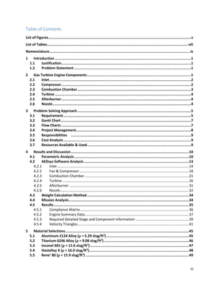
in a plate with a thickness ranging up to six inches. It can be seen in Figure 5.1 below the traditional yield
and ultimate tensile strength data for Aluminum 2124. The figure will allow for a non-conservative design
to be considered because of the fact that the part could undergo permanent deformation during the
exposure time.
Figure 5.1: Effect of Temperature and Exposure Time on Tensile Properties
It is actually preferable to base designs on creep and creep-rupture data. The values for these can be
determined by using Figure 5.2. For common practice, an allowance of less than 1% creep during the life
of the part. As seen in the figure, Al 2124 is seldom used above 400˚F. From the figure, it should be noted
that reductions will be made to results because of the cyclic stress, uncertainties in load calculations,
property variations, and safety margins. Based on the properties seen in the figures and recently stated,
the inlet and nacelle will be using Al 2124.

57. 46
Figure 5.2: Creep and Creep-rupture curves at temperatures from 75 to 600˚F for 2124-T851 plate
5.2 Titanium 6246 Alloy (ρ = 9.08 slug/ft3
)
This alloy was designed to combine long-time, elevated-temperature strength characteristics with
markedly improved short-time strength properties at both room and elevated temperatures. It is intended
for use in forging for intermediate-temperature-range sections of gas turbine engines, particularly in
stator and rotor airfoil components of the fan and compressor.
Ti-6246 is recommended for gas turbine applications up to 750˚F. Figure 5.3 below can be seen to compare
the allowable stress based on the needed temperature applications based on 1% creep for 1000 hours. It
can also be seen that Ti-6246 allows for regulated cyclic stress. It also has a poor fracture toughness and
is very susceptible to minor damage. Therefore, it is recommended to use a damage-tolerant processed
version of Ti-6246.
Figure 5.3: Axial Fatigue Properties of α-β forged materials in two heat-treated conditions

58. 47
5.3 Inconel 601 (ρ = 15.6 slug/ft3
)
This is a general-purpose alloy for applications requiring resistance to both heat and corrosion at
temperatures up to about 2100˚F. It has been used in burner liners, diffuser assemblies, containment
rings, exhaust liners, and burner igniters. The data shown in Figure 5.4 below can be used to compare the
stresses based on a 1% creep rate. In contrast to the titanium alloy listed above, Inconel 601 retains much
of its room temperature strength well beyond 1000˚F. Figure 5.5, seen below, also displays that it has
more than adequate fatigue strength when considering vibrations. Due to these properties, it is suggested
that most components of the combustion chamber and afterburner use Inconel 601.
Figure 5.4: Minimum creep rate at various temperatures and stresses
Figure 5.5: Fatigue properties of annealed sheet

59. 48
5.4 Hastelloy X (ρ = 16.0 slug/ft3
)
This is a nickel-base superalloy with good oxidation resistance at temperatures up to 2200˚F. It has been
used in jet engine exhaust nozzles, afterburner components, and structural parts in the burner and turbine
components. By referring to Figure 5.6 below, the stresses can be found at certain temperatures based
on the amount of creep allowable for the component.
Figure 5.6: Creep-deformation curves for plate and bar at temperatures of 1200-1800˚F
Because Hastelloy X is generally used in situations where only low-cycle fatigue caused by pressure or
thermal cycles matters, its fatigue characteristics are presented in terms of strain range rather than stress
range. It can be seen in Figure 5.7 below how the material will react in cycles of use.
Figure 5.7: Fatigue life of plate at various temperatures in air and impure helium at atmospheric pressure
The modulus of elasticity given in Figure 5.8 below can also be used to obtain the thermal stress
calculation involved. Note that in the 1200-1600˚F range, the modulus of elasticity is approximately 20

60. 49
million psi. Consequently, the stress corresponding to a 1% strain range equates approximately to 200,000
psi. This makes it evident that such materials can tolerate only a small fraction of a percent strain.
Figure 5.8: Effect of elevated temperature on modulus of elasticity
5.5 Rene’ 80 (ρ = 15.9 slug/ft3
)
This is a cast, precipitation-hardenable, nickel-base superalloy. It has excellent creep-rupture strength up
to 1900˚F, combined with good elevated temperature ductility and superior hot corrosion resistance. The
main use of Rene’ 80 is in investment-vacuum-cast turbine stator and rotor airfoils, which are coated for
any jet engine application. Using the 1% creep deformation at the 1000-hour criterion, Figure 5.9 below
reveals that Rene 80’ has a remarkably high tensile stress capability.
Figure 5.9: Creep Strain and creep-rupture at 1400, 1600, and 1800˚F for fully treated cast alloy
Alternating stress conditions are often important in cooled turbine rotor airfoils, which are usually
cantilevered and subject to the aerodynamic buffeting that produces vibratory loads. It is especially

61. 50
important to avoid resonance between a regular upstream disturbance and a natural frequency of the
rotor airfoils. Thermal stresses can cause low-cycle fatigue failure if the limits given in Figure 5.10 are
reached. This means that cooled airfoils must be designed with the greatest care so that no local areas of
large thermal stress are created at any time during the normal engine operation. In particular, it can be
readily seen that a thin airfoil “skin” with a large temperature difference between coolant and mainstream
will not last long.
Figure 5.10: Axial Low Cycle Fatigue behavior at 1200-1800˚F

62. 51
6 Conclusion
Upon completion of the DKA-867 components, it was found that the engine had achieved each objective
set out by AIAA. To begin, the thrust of the newly designed low-bypass turbofan is able to achieve the
needed thrusts for takeoff, loiter, cruise, and supersonic burst at each given flight condition. The thrusts
acquired is also higher than that defined by the baseline turbojet engine. Fuel consumption was also
lowered for each individual flight condition. The maximum defined fuel consumption was lowered well
beyond the point needed for both wet and dry conditions. This allows for a highly efficient engine to be
used on the T-38 Talon. With this comes a lowered cost of flight. The next two requirements set out by
AIAA was to stay within certain dimensions and weight for the engine without the afterburning section.
The dimensions for both the length of engine less afterburner and fan diameter were kept within the
specifications. In fact, the length of the engine is smaller than that of the baseline turbojet engine. Due to
the smaller length, the engine weight has also been lowered compared to the baseline turbojet engine.
It can be seen that the DKA-867 afterburning low-bypass turbofan engine will be more efficient for any
flight condition of the T-38. Therefore, the DKA-867 will offer an excellent substitute for the already in use
J85-GE-5A afterburning turbojet engine. Since the low-bypass turbofan engine is shorter than the
turbojet, an easy swap can be made. An inlet for the DKA-867 has been made based on the specifications
required by AIAA. Although the engine can be easily added to the T-38, the alternate design of the inlet
will cause for a new nacelle design which will need to be replaced on the T-38 as well. Upgrades have also
been made to the material choice in each component of the DKA-867. The new material choice will also
cause an increase in engine cost. The engine will be able to have less maintenance hours due to the
increased stress and creep tolerances. Along with cooling to be used in the turbine blades, combustion
chamber, and afterburner, the engine will be able to last many more hours than the baseline turbojet
engine.
To finalize the design of the DKA-867 afterburning low-bypass turbofan engine results, a complete
computational fluid dynamic, finite element analysis, and physical testing of a prototype engine must be
made. Due to time restraints and being outside the scope of this project, such results were not found. By
using each individual test, the validity of the results using the AEDsys software can be found. Upon
completion of the tests previously mentioned, FAA regulations must be taken into consideration. When
calculating the design of each component of the DKA-867, the regulations have been taken into
consideration. The design calculations may not always prove to be as precise as actual testing. Therefore,
a list of the regulations for FAA can be found by following the websites listed in the References section of
this report. After completion of each test and obtaining authorization from FAA, the engine will then be
ready for flight.

63. 52
7 References
[1] J. D. Mattingly, Elements of Propulsion: Gas Turbines and Rockets, 1st Edition ed., J. A. Schetz, Ed.,
Reston, Virginia: AmericanInstituteof Aeronauticsand Astronautics,Inc., 2006.
[2] J. D. Mattingly, Aircraft Engine Design, 2nd Edition ed., J. S. Przemieniecki, Ed., Reston , VA: American
Institute of Aeronautics and Astronautics , 2002.
[3] H. R. &. D. Mavris, "Preliminary Design of a 2D SUpersonic Inlet to Maximize Total Pressure Recovery".
[4] J. L. Kerrebrock, Aircraft Engines and Gas Turbines, Massachusetts: The Alpine Press Inc. , 1977.
[5] C. W. Smith, Aircraft Gas Turbines, New York : John Wiley & Sons , 1956.
[6] FAA, "14 CFR Parts Applicable to Engines & Propellers," 22 March 2016. [Online]. Available:
https://www.faa.gov/aircraft/air_cert/design_approvals/engine_prop/engine_prop_regs/regs/ .
[Accessed 10 April 2016].

64. 53
8 Appendix A: Acknowledgements
We would like to thank multiple people in aiding us complete this project in an orderly and timely manner.
To begin, our advisor and mentor Dr. Adeel Khalid has been with us every step of the way. We would like
to thank him for taking time out of his schedule in order to help us succeed. He has spent time reviewing
the calculations and pointing us in the correct direction when it seemed there was none. His expertise in
engine design has been of great use when questions were posed. Along with Dr. Khalid, a series of videos
posted by Agent Jay-Z have been of great help in understanding the component design. With his videos,
many of the unknowns were able to be known. He currently works in a turbine engine repair shop and
develops movies of the incoming engines. By dissecting each component, we have been able to visually
understand the geometry. Finally, the staff at Starbucks off of highway 120 has been of great courtesy.
They have consistently allowed us to use their space in aid of completing our project. Along with this, they
have offered free coffee and questioning of our project. Without them being open, we would not have
been able to meet at sometimes in-opportune hours of the morning and night.

65. 54
9 Appendix B: Contact Information
David Byrd
Email: 57tbyrd@gmail.com
Phone: (678) 447-4729
Kristian Lien
Email: Kristian0662@gmail.com
Phone: (678) 777-3761
Austin Sims
Email: austinsims@bellsouth.net
Phone: (678) 296-5514

66. 55
10 Appendix C: Reflections
David Byrd:
This project has been the most challenging yet interesting task of my college career. I have always had a
love for engines and trying to make them more powerful. When AIAA posed a competition to design a
low-bypass turbofan engine using a baseline turbojet engine, I knew this was the project for me.
Fortunately, I found two other people with the same passion for air, fuel, and power. The three of us set
out to design the best low bypass engine we could as well as furthering our understanding of gas turbine
engine.
Upon starting the project, I decided that I would take on the responsibility of designing the compressor
and the afterburner. Little did I know how complex and vital the compressor was to the entire engine.
With the use of “Aircraft Engine Design Second Edition” [2] and “Elements of Propulsions: Gas Turbines
and Rockets” [1] books, I was able to increase my knowledge of the in-depth calculations for each stage
of the compressor. Using the process found in both books, I generated an Excel spreadsheet for each stage
of the compressor. This task turned into a considerable greater undertaking. Even though the Excel
spreadsheet did not work the way anticipated, it did increase my understanding of the relationship with
the values in the compressor. I took most of the values found in the Excel spreadsheet and input the into
COMPR program. The output data allowed me to double check my initial calculations and provided other
critical data for the compressor. After main iterations of the Excel spreadsheet and the COMPR program,
the compressor was finally completed.
One of the major disadvantages of designing the afterburner, was the lack of useful resources. “Aircraft
Engine Design Second Edition” [2] used a combination of ONX, GASTAB, AFTRBRN program to design the
afterburner. I initial started an Excel Spreadsheet, but reverted to the process describe in “Aircraft Engine
Design Second Edition” [2] book due to absence of information. However, the process in the book was
not the easiest to follow, but did produce excellent results. This Project has been a great challenge to me
while sheading knowledge of the complexity of a gas turbine engine. I would like to thank Dr. Adeel Khalid
for his time teaching and a growing my love of the aerospace engineering.
Kristian Lien:
Upon beginning the engine design project, I knew it would be a great challenge. It soon became one of
the hardest things I had done in school but also my greatest success. Upon taking the Aircraft Propulsion
class, I knew that my calling would be to design engines for a living. To challenge that goal, my group and
I decided to design a propulsive system for our Aeronautics Senior Design Project. Luckily, AIAA had posed
a competition to design a low-bypass turbofan engine using a baseline turbojet engine. This helped in the
ease of knowing what to expect for results as well as comparison purposes. In beginning the project, each
component had to be designated to each group member.
I had decided to design the turbine as well as the combustion chamber. Initially, I knew that the design of
both would be quite perplexing. To obtain more knowledge about each individual system, much research
and reading was done. By using both the “Aircraft Engine Design Second Edition” [2] and “Elements of
Propulsions: Gas Turbines and Rockets” [1] books, much new knowledge was obtained on either subject.
To begin, the turbine had to be developed. Using the equations found in each book, an Excel spreadsheet
was created. The results of the spreadsheet created little success but helped with an understanding of
how each input value could determine the resulting flow through the turbine. After weeks of

67. 56
manipulation, the TURBN program was used to finalize the design. It took many iterations using the
program to achieve the needed results for each stage but proved to be easier than the spreadsheet. Upon
obtaining values of the turbine size, the combustion chamber then needed to be designed. As seen in the
turbine, an excel spreadsheet was created to visualize and understand the complexity of the combustion
chamber. After many revisions, the MAINBRN program was used to finalize the design of the combustion
chamber. The manipulation of the diffuser and primary zone seemed to pose the greatest difficulty.
Through many iterations, a desired size, number of secondary and dilution zone holes, and temperatures
were obtained. Once completing the designs, a time for reflection on accomplishments was needed.
It was stated that a huge learning curve was needed for both the understanding of component design and
program use. Luckily, the books my group and I had used aided in both. It took countless hours of reading
chapters to fully understand the preliminary design of the turbine and combustion chamber. It took even
longer to appreciate how much each individual component affects the others. As stated previously, many
iterations were made to obtain desired goals. Occasionally, when the components neared completion, it
was found that other components in the engine needed to be reassessed. This caused a new design
needed for both combustion chamber and turbine. The overall design posed a great challenge but allowed
for my dream to become an engine designer to reach a new height. Understanding the complexity of each
engine stage allowed for a greater sense of accomplishment as an individual. With the help of our
advisor/mentor Dr. Adeel Khalid and the books written by Jack D. Mattingly, a higher appreciation of
propulsive systems was accomplished.
Austin Sims:
The decision to take on this project is something I do not regret. In my mechanical and aeronautical
engineering studies, my proficiency relative to thermodynamics and heat transfer has been one of my
weaknesses. Knowing this, I chose to see this as an opportunity to not only challenge me but to better
myself as engineer. One thing I have learned in my studies is that with enough work and determination I
can do just about anything. Sure enough once getting into the project my previous knowledge learned
and experiences with preliminary engine design in my classes helped guide me along the way.
The engine components I chose to design for this project included the 2-Ramp External Compression Inlet
with a Diffuser and the Convergent-Divergent Nozzle. Initially I knew that a great deal of work and effort
went in to the development of these two elements. What I learned very quickly is that it’s one thing to
design the sections individually, but it’s another to design them so that they are optimally in tune with the
entire engine. This can be seen considering one of my main references used for this project is an entire
paper on the optimization of a 2-D ramped external compression inlet. For the purposes and general scope
of this project the designs of my components include a fixed geometry for the inlet and the optimized
convergent-divergent angles of the nozzle for only the aircraft’s main flight conditions. In cases like the F-
14 and the Concorde their inlet and nozzle geometries vary relative to the aircraft’s different flight
conditions midflight. Ultimately there is an unlimited number of combinations in which the geometries
can be arranged for every possible flight condition. Recognizing the true scope of the project as a
preliminary engine design, much of my information and influence for design came from the use of two of
my textbooks by Jack D. Mattingly: “Aircraft Engine Design, Second Edition” and “Elements of Propulsion:
Gas Turbines and Rockets.” Using these resources helped me to organize a better plan of attack and more
efficiently determine the best possible results and performance of the engine components while
minimizing their vast complexities that could be investigated.

68. 57
In correlation with the text resources, the use of the AEDsys software and its INLET and NOZZLE programs
helped to expedite the process of calculating the design performance and component sizing of each
component. Additionally, the computations based on a given mission leg could be completed in order to
enhance the comprehensive performance of each component. The fundamental results found for the inlet
were the total pressure recovery, the eventual velocity at the fan face, and the capture area sizing suitable
for obtaining the mass flow rate required by the engine. Similarly, the significant products of the nozzle
include the gross thrust actual produced at exit, the exit velocity of the air flow, and pressure matching at
the nozzles exit. Considering these aspects of the design, the losses and flow separation are supposed to
be limited.
After experiencing the intricacies in the research, design, and development required by this project I
learned a great deal about myself. At first it seemed as if taking on this project would be virtually
impossible given the groups initial knowledge of the subject and time limitations of a heavy class load. In
the end tenacity and not accepting nothing less than success prevailed. I will be able use this experience
in the future as a baseline of what I should expect myself being able to accomplish. As student at the end
of my college career this has helped me to boost my confidence and resolve when faced with adversity.
Furthermore, the knowledge gained from my studies, my mentor/advisor Dr. Adeel Khalid, and this
project will be a strong foundation for me as I embark onto my professional career and future endeavors.

69. 58
11 Appendix D: Initial Values and Requirements
11.1 Inlet
Table 11.1: Table of Initial Value for Inlet
Initial Values
Selected Shock System Required Selected Resulting
M0 ηR As/A0i A0 (ft2
) A0i (ft2
) As (ft2
) A1 (ft2
) As (ft2
) A0i (ft2
)
Fgc
ṁ 0a0
φinlet
1.0 1.0000 1.0000 2.874 3.012 3.012 4.000 3.203 3.203 3.500 0.0000
1.1 0.9989 0.9995 2.896 3.046 3.045 4.000 3.203 3.205 3.522 0.0025
1.2 0.9928 0.9990 2.944 3.109 3.106 4.000 3.203 3.206 3.542 0.0041
1.3 0.9972 0.9453 3.062 3.246 3.068 4.000 6.203 3.388 3.560 0.0073
1.4 0.9896 0.9290 3.179 3.382 3.142 4.000 3.203 3.447 3.576 0.0076
1.5 0.9947 0.8635 3.372 3.640 3.124 4.000 3.203 3.732 3.590 0.0111
Table 11.2: Table of Requirements for Inlet
Requirements
Inlet Requirements Based on Engine
Performance Cycle Analysis Calculations
Inlet Area Modified for Safety
Margin and Boundary Layer Bleed
M0 ηR spec A0 spec (ft2
) A0 spec + 4% (ft2
) A0t spec (ft^2)
1.0 1.0000 2.874 2.989 3.012
1.1 0.9966 2.889 3.005 3.039
1.2 0.9915 2.940 3.058 3.105
1.3 0.9852 3.025 3.146 3.207
1.4 0.9782 3.142 3.268 3.343
1.5 0.9706 3.290 3.422 3.514
11.2 Fan/Compressor
Table 11.3: Initial Values and Requirements for Fan/Compressor
Initial Values Requirements
Low Pressure/Fan High Pressure Low Pressure/Fan High Pressure
M1 = M3 60˚F ≤ ΔTt per stage ≤ 100˚F 60˚F ≤ ΔTt per stage ≤ 90˚F
α1 = α1 = 40 deg 1.5 ≤ πc for one stage ≤ 2.0 0.90 ≤ Hub/tip at exit ≤ 0.92
u2/u1 = 1.1 2.0 ≤ πc for two stage ≤ 3.5 1300 ft
/s ≤ Vrim exit ≤ 1500 ft
/s
Φcr = 0.09 3.5 ≤ πc for three stage ≤ 4.5 1700 R ≤ Max Texit ≤ 1800 R
Φcs = 0.03 0.50 ≤ DF ≤ 0.55
σ = 1.0 1400ft
/s ≤ Vtip ≤ 1500 ft
/s
c/h = 0.5

70. 59
11.3 Combustion Chamber
Table 11.4: Initial Values and Requirements for Combustion Chamber
Initial Values Requirements
ηDm = 0.9 0.2 ≤ φ ≤ 1.0
θ = 5 deg 0.6 ≤ S' ≤ 1
ε = 1 35 deg ≤ αSW ≤ 50 deg
Tm = 2500 R 3000 R ≤ Tg ≤ 3420 R
rh = 0.5 in φPZ ≥ 0.8
αSW = 45 deg εPZ ≈ 0.7
ri ≥ 0.5 in.
11.4 Turbine
Table 11.5: Initial Values and Requirements for Turbine
Initial Values Requirements
High Pressure Low Pressure High Pressure Low Pressure
M2 = 1.1 M2 = 0.9
4x1010
in2
-rpm2
≤ AN2
≤
4x1010
in2
-rpm2 N/A
α1 = 0 deg 1.4 ≤ Ψ ≤ 2.0 Ψ ≤ 2.4
u3/u2 = 0.9 0.4 ≤ M3 ≤ 0.5
φt stator = 0.06 0 deg ≤ α3 ≤ 40 deg
φt rotor = 0.15 0.3 ≤ c/h ≤ 1.0
Z = 1.0 Best performance : 60 deg ≤ α2 ≤ 70 deg
c/h = 1.0 Mean radius (rm) stays consitient
σ = 1.0

71. 60
11.5 Afterburner
Figure 11.1: Principal Features and Flow Patterns of the Afterburner

72. 61
11.6 Nozzle
Figure 11.2: Nozzle Discharge Coefficient: b) Convergent and C-D Nozzle CD max

73. 62
Figure 11.3: C-D Nozzle Velocity Coefficient

74. 63
Figure 11.4: C-D Nozzle Angularity Coefficient

75. 64
12 Appendix E: ONX Parametric Analysis
12.1 Mach 0 and Sea Level
Figure 12.1: ONX Parametric Analysis Results at M=0 and Sea Level

76. 65
Figure 12.2: Preliminary Engine Performance Analysis at M=0 and Sea Level

77. 66
12.2 Mach 0.5 and 15,000 feet
Figure 12.3: ONX Parametric Results at M=0.5 and 15,000 feet

78. 67
Figure 12.4: Preliminary Engine Performance Analysis at M=0.5 and 15,000 feet

79. 68
12.3 Mach 0.85 and 35,000 feet
Figure 12.5: ONX Parametric Analysis Results M=0.85 and 35,000 feet

80. 69
Figure 12.6: Preliminary Engine Performance Analysis at M=0.85 and 35,000 feet

81. 70
12.4 Mach 1.3 and 40,000 feet
Figure 12.7: ONX Parametric Analysis Results at M=1.3 and 40,000 feet

82. 71
Figure 12.8: Preliminary Engine Performance Analysis at M=1.3 and 40,000 feet

83. 72
13 Appendix F: AEDsys Test Data
13.1 Inlet
Figure 13.1: Inlet Inputs and Results

84. 73
Figure 13.2: Inlet Side View
Figure 13.3: Inlet Angle Contours
13.2 Fan/Compressor
13.2.1 Inlet Guide Vanes
13.2.1.1 Low Pressure
Figure 13.4: Low Pressure IGV Results

85. 74
Figure 13.5: Low Pressure IGV Blade Profile
13.2.1.2 High Pressure
Figure 13.6: High Pressure IGV Results
Figure 13.7: High Pressure IGV Blade Profile

86. 75
13.2.2 Fan/Low Pressure Compressor
Figure 13.8: Fan/Low Pressure Compressor Layout
13.2.2.1 Stage One
Figure 13.9: Low Pressure Stage 1 Results

87. 76
Figure 13.10: Low Pressure Stage 1 Blade Profile
13.2.2.2 Stage Two
Figure 13.11: Low Pressure Stage 2 Results

88. 77
Figure 13.12: Low Pressure Stage 2 Blade Profiles
13.2.2.3 Stage Three
Figure 13.13: Low Pressure Stage 3 Results

89. 78
Figure 13.14: Low Pressure Stage 3 Blade Layout
13.2.3 High Pressure Compressor
Figure 13.15: High Pressure Compressor Layout

90. 79
13.2.3.1 Stage One
Figure 13.16: High Pressure Stage 1 Results
Figure 13.17: High Pressure Stage 1 Blade Layout

91. 80
13.2.3.2 Stage Two
Figure 13.18: High Pressure Stage 2 Results
Figure 13.19: High Pressure Stage 2 Blade Profile

92. 81
13.2.3.3 Stage Three
Figure 13.20: High Pressure Stage 3 Results
Figure 13.21: High Pressure Stage 3 Blade Profile

93. 82
13.2.3.4 Stage Four
Figure 13.22: High Pressure Stage 4 Results
Figure 13.23: High Pressure Stage 4 Blade Profile

94. 83
13.2.3.5 Stage Five
Figure 13.24: High Pressure Stage 5 Results
Figure 13.25: High Pressure Stage 5 Blade Profile

95. 84
13.3 Combustion Chamber
Figure 13.26: Data Entry for Combustion Chamber
Figure 13.27: Air Partitioning for Combustion Chamber

96. 85
Figure 13.28: Diffuser for Combustion Chamber
Figure 13.29: Primary Zone for Combustion Chamber

97. 86
Figure 13.30: Secondary Zone for Combustion Chamber
Figure 13.31: Dilution Zone for Combustion Chamber

98. 87
Figure 13.32: Combustion Chamber Front View
Figure 13.33: Combustion Chamber Side View

99. 88
Figure 13.34: Combustion Chamber Plan View
13.4 Turbine
13.4.1 High Pressure Turbine
Figure 13.35: High Pressure Results

100. 89
Figure 13.36: High Pressure Layout
Figure 13.37: High Pressure Blade Layout
13.4.2 Low Pressure Turbine
Figure 13.38: Low Pressure Results

101. 90
Figure 13.39: Low Pressure Layout Figure 13.40: Low Pressure Blade Layout
13.4.3 Exit Guide Vanes
Figure 13.41: Exit Guide Vane Results
Figure 13.42: Exit Guide Vane Results

102. 91
13.5 Afterburner
Figure 13.43: Data Entry
Figure 13.44: Data Entry
Figure 13.45: Flameholders

103. 92
Figure 13.46: Side View of Afterburner
13.6 Nozzle
13.6.1 Mach 0
Figure 13.47: Nozzle Input and Results at Mach 0

104. 93
Figure 13.48: Divergent Angle Contours at Mach 0
Figure 13.49: Nozzle Side View at Mach 0
13.6.2 Mach 0.5
Figure 13.50: Nozzle Input and Results at Mach 0.5
Figure 13.51: Divergent Angle Contours at Mach 0.5
Figure 13.52: Nozzle Side View at Mach 0.5

105. 94
13.6.3 Mach 0.85
Figure 13.53: Nozzle Input and Results at Mach 0.85
Figure 13.54: Divergent Angle Contours at Mach 0.85
Figure 13.55: Nozzle Side View at Mach 0.85
13.6.4 Mach 1.3
Figure 13.56: Nozzle Input and Results at Mach 1.3

106. 95
Figure 13.57: Divergent Angle Contour at Mach 1.3
Figure 13.58: Nozzle Side View at Mach 1.3
13.7 Mission Analysis Results
Figure 13.59: Warm-Up Leg

107. 96
Figure 13.60: Takeoff Accelerate
Figure 13.61: Takeoff Rotation

108. 97
Figure 13.62: Horizontal Acceleration
Figure 13.63: First Climb and Acceleration

109. 98
Figure 13.64: Second Climb and Acceleration
Figure 13.65: Third Climb and Acceleration

110. 99
Figure 13.66: Subsonic Cruise
Figure 13.67: Climb and Accelerate to Supersonic Cruise

111. 100
Figure 13.68: Supersonic Cruise
Figure 13.69: Descend to Subsonic Cruise

112. 101
Figure 13.70: Subsonic Cruise
Figure 13.71: Descend to Loiter

113. 102
Figure 13.72: Loiter
Figure 13.73: Descend to Land

114. 103
Figure 13.74: Results of Mission