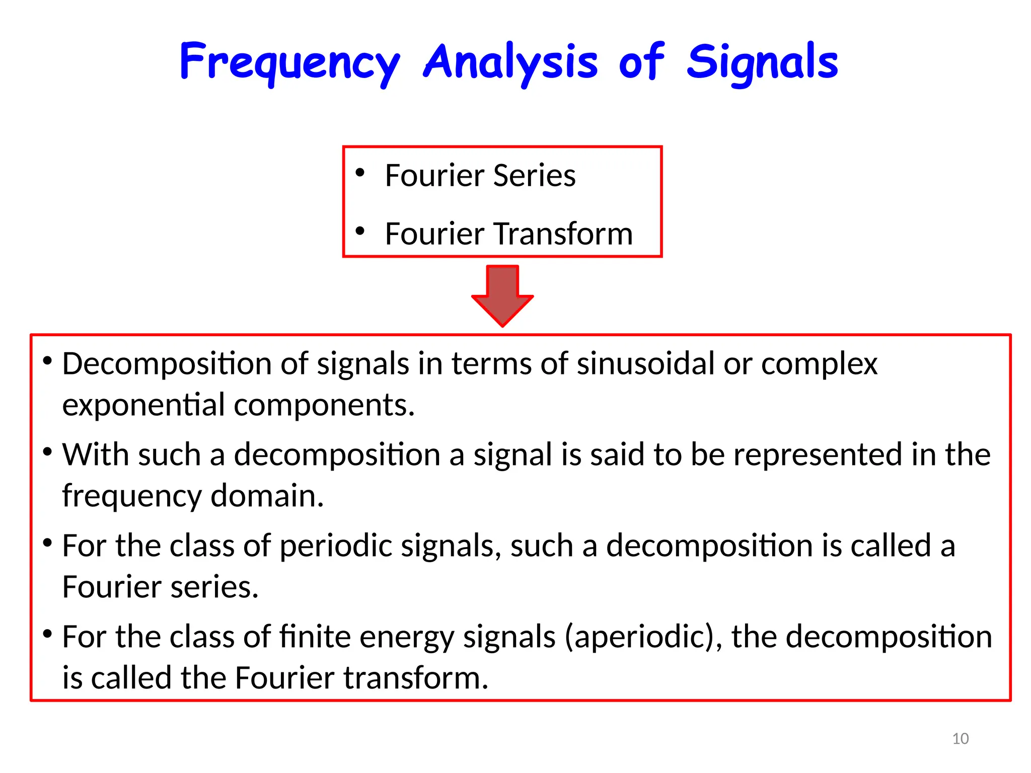
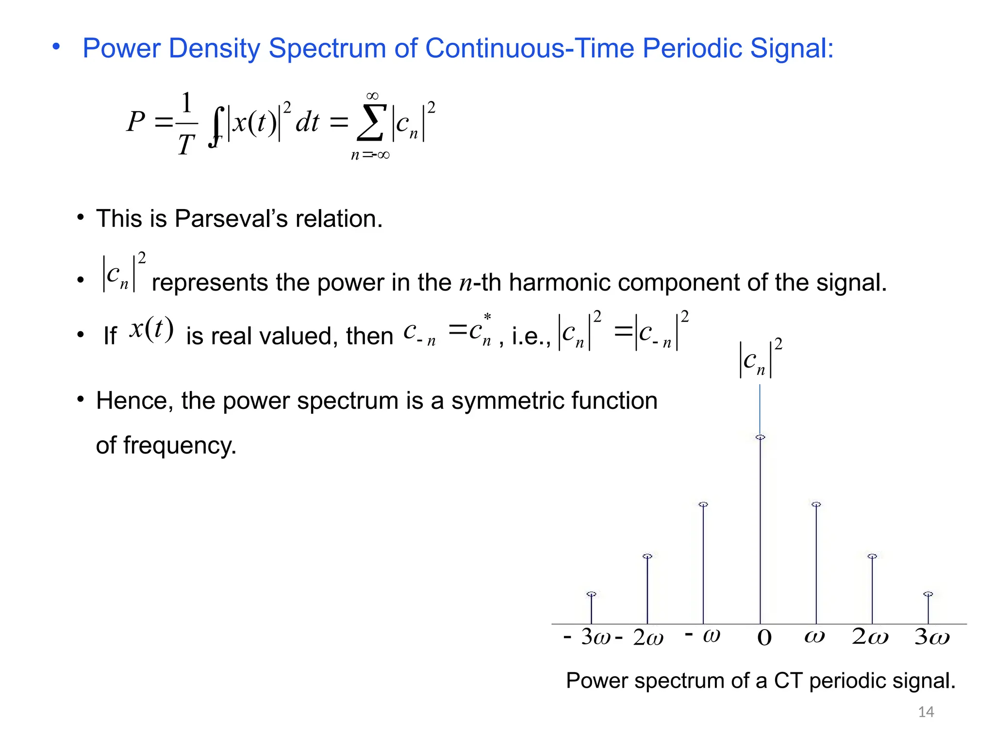
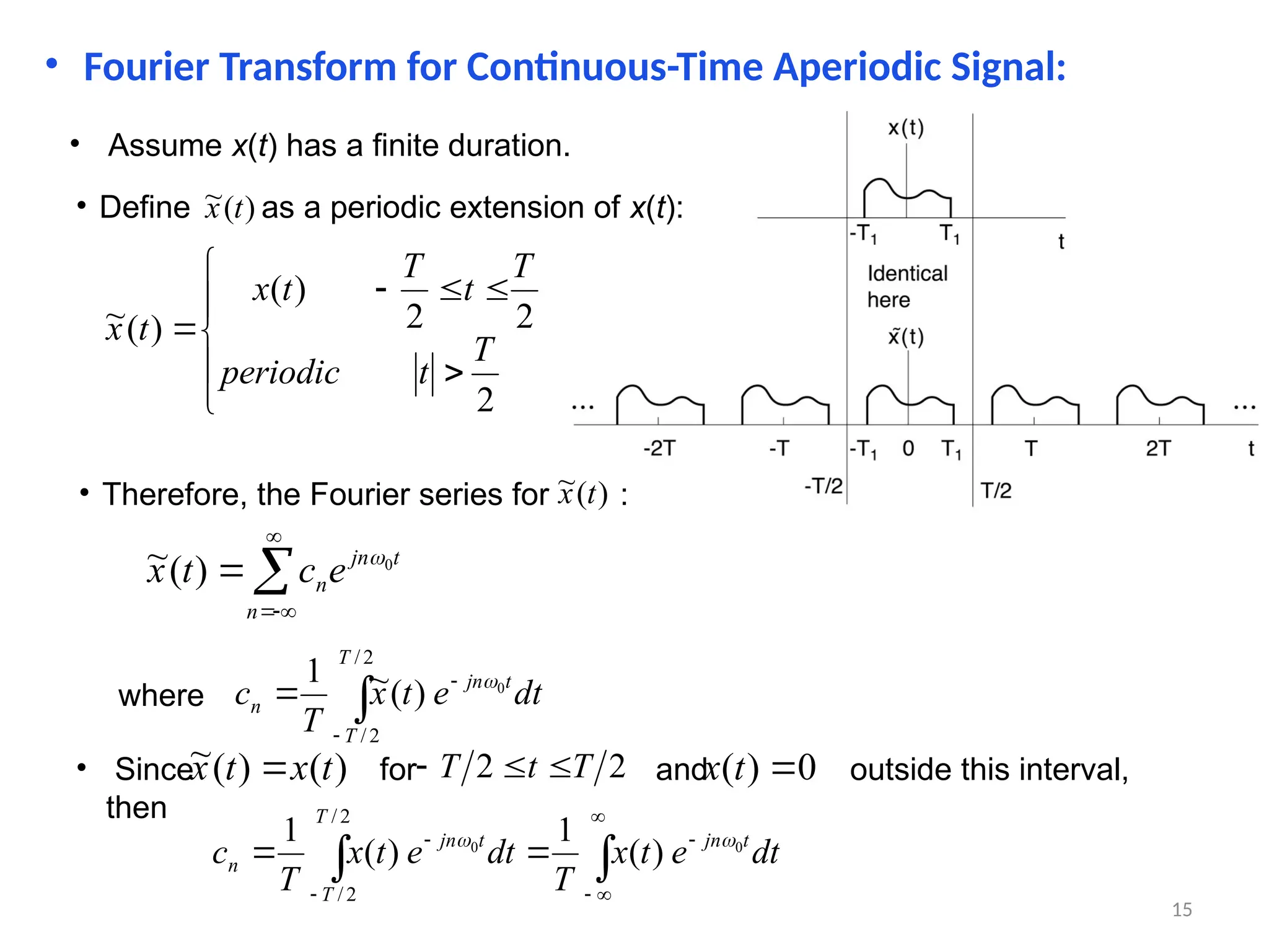
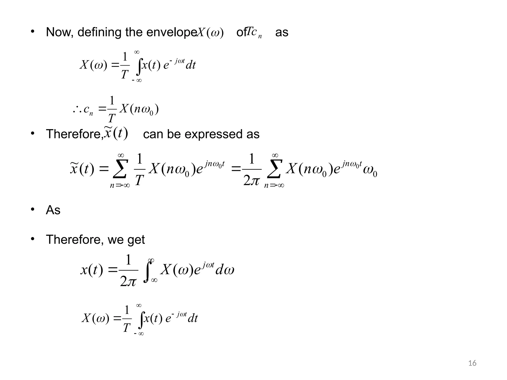
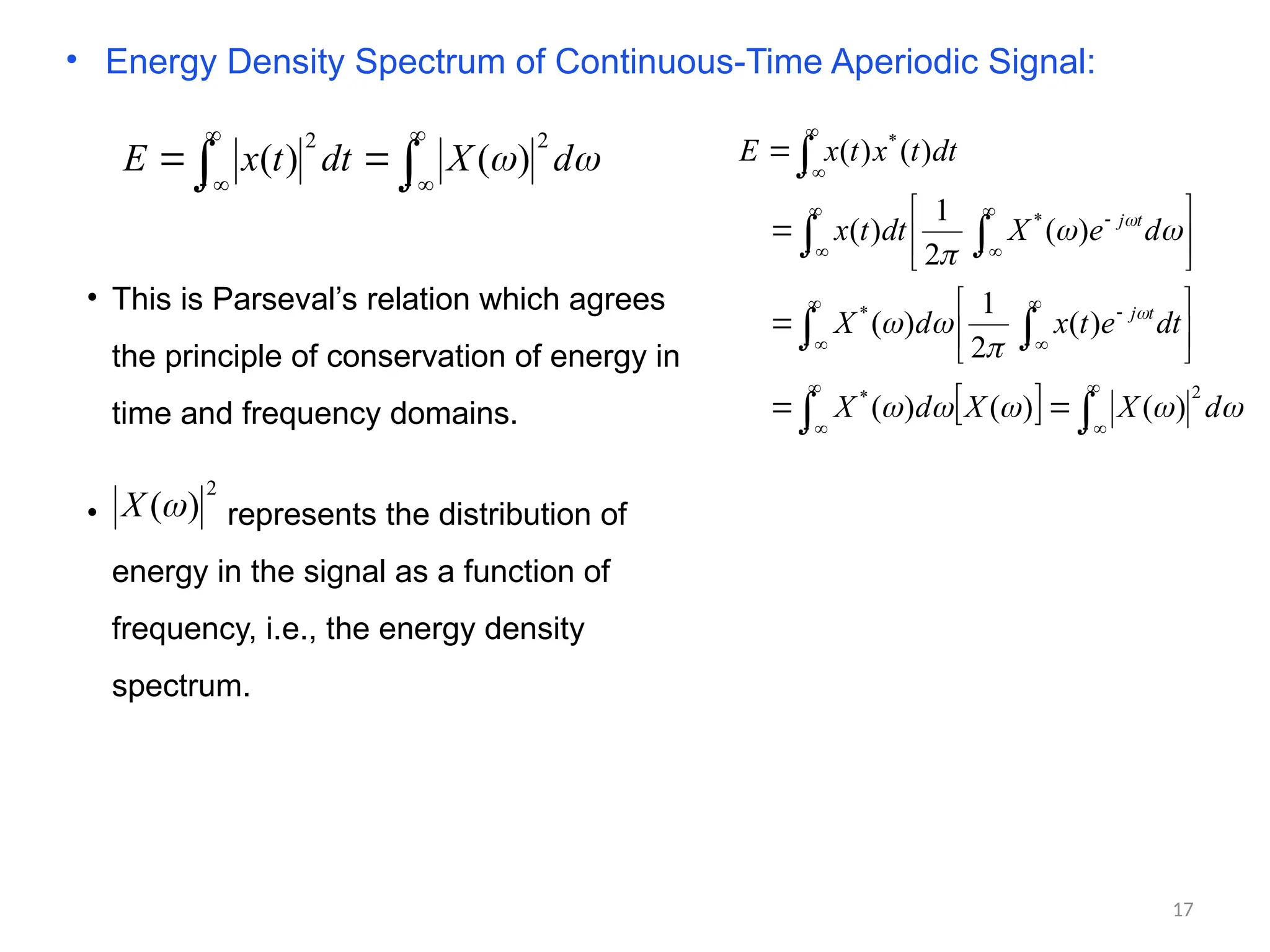
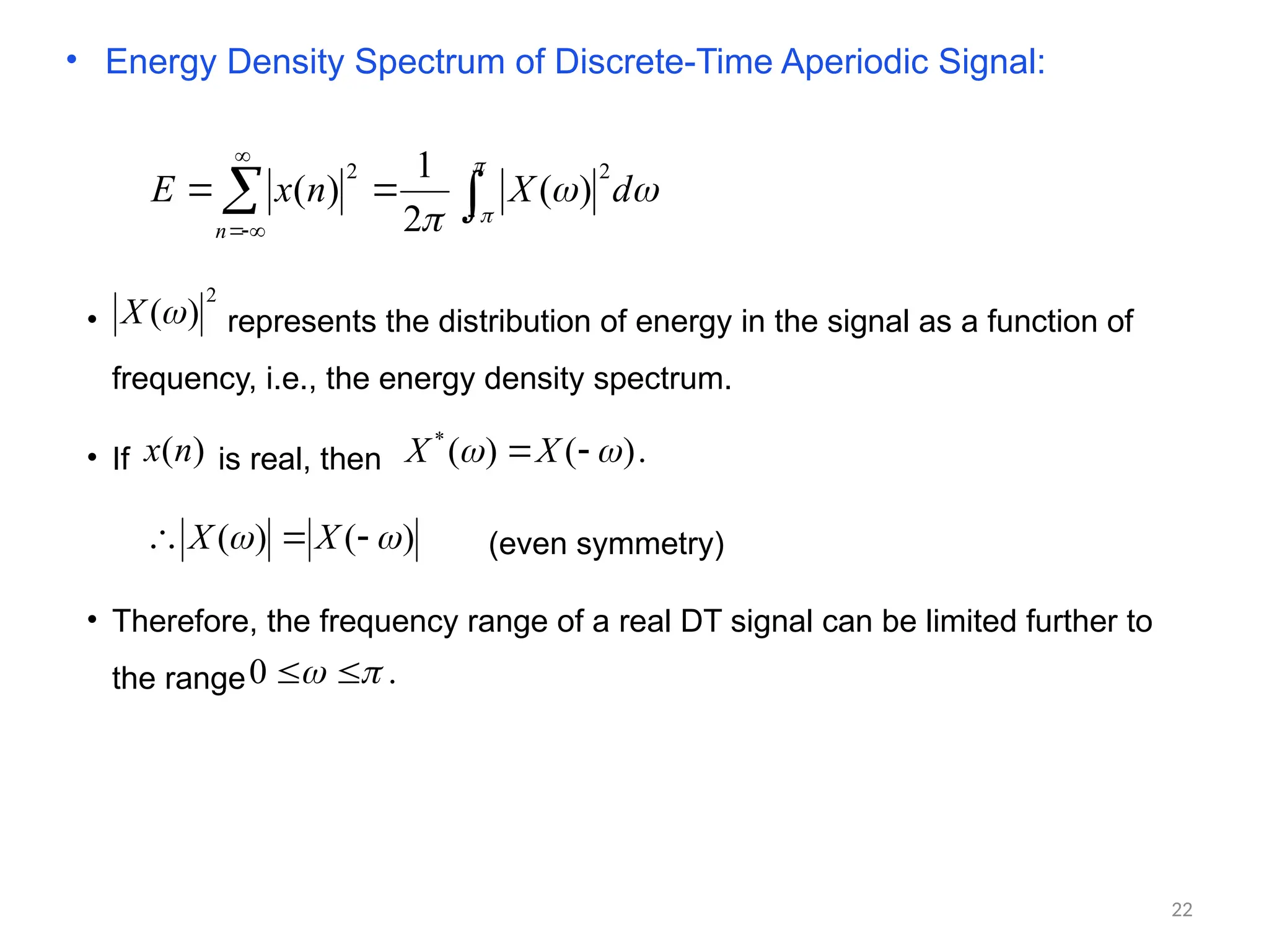
The document provides an overview of Fourier analysis in the context of signals and linear time-invariant (LTI) systems, detailing properties, mathematical representations, and applications. It discusses the response of LTI systems to various signals, highlighting the importance of convolution and the characterization of systems by their impulse responses. Additionally, it explains Fourier series and Fourier transforms for both continuous and discrete-time signals, including energy density spectra and the conservation of energy in time and frequency domains.

1. Fourier Analysis of Signals
and
Systems
Dr. Babul Islam
Dept. of Applied Physics and Electronic
Engineering
University of Rajshahi
1

2. Outline
• Response of LTI system in time domain
• Properties of LTI systems
• Fourier analysis of signals
• Frequency response of LTI system
2

3. • A system satisfying both the linearity and the time-
invariance properties.
• LTI systems are mathematically easy to analyze and
characterize, and consequently, easy to design.
• Highly useful signal processing algorithms have been
developed utilizing this class of systems over the last
several decades.
• They possess superposition theorem.
Linear Time-Invariant (LTI) Systems
3

4. • Linear System:
+ T
)
(
1 n
x
)
(
2 n
x
1
a
2
a
 
]
[
]
[
)
( 2
2
1
1 n
x
a
n
x
a
n
y 
T
   
]
[
]
[
)
( 2
2
1
1 n
x
a
n
x
a
n
y T
T 


+
)
(
1 n
x
)
(
2 n
x
1
a
2
a
T
T
System, T is linear if and only if
i.e., T satisfies the superposition principle.
)
(
)
( n
y
n
y 

4

5. • Time-Invariant System:
A system T is time invariant if and only if
)
(n
x T )
(n
y
implies that
)
( k
n
x  T )
(
)
,
( k
n
y
k
n
y 

Example: (a)
)
1
(
)
(
)
(
)
1
(
)
(
)
,
(
)
1
(
)
(
)
(














k
n
x
k
n
x
k
n
y
k
n
x
k
n
x
k
n
y
n
x
n
x
n
y
Since )
(
)
,
( k
n
y
k
n
y 
 , the system is time-invariant.
(b)
]
[
)
(
)
(
]
[
)
,
(
]
[
)
(
k
n
x
k
n
k
n
y
k
n
nx
k
n
y
n
nx
n
y







Since )
(
)
,
( k
n
y
k
n
y 
 , the system is time-variant. 5

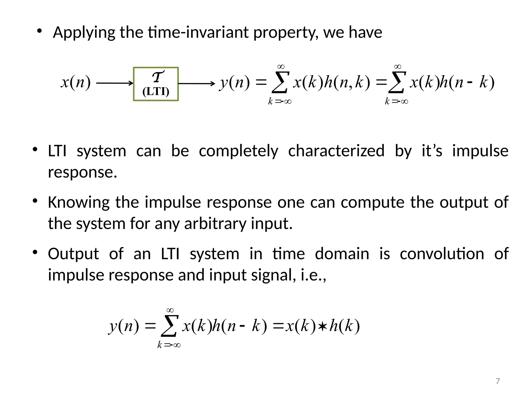
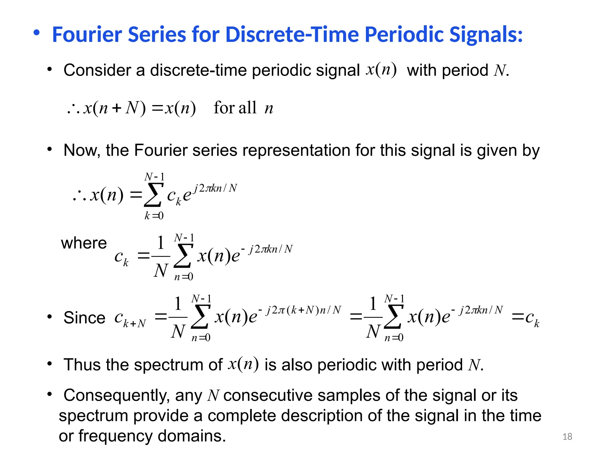
6. • Any input signal x(n) can be represented as follows:






k
k
n
k
x
n
x )
(
)
(
)
( 
• Consider an LTI system T.
1






0
for
,
0
0
for
,
1
]
[
n
n
n

0 n
1 2
-1
-2 …
…
Graphical representation of unit impulse.
)
( k
n 
 T )
,
( k
n
h
)
(n
 T )
(n
h
• Now, the response of T to the unit impulse is
)
(n
x T   )
,
(
)
(
]
[
)
( k
n
h
k
x
n
x
n
y
k





T
• Applying linearity properties, we have
6

7. • LTI system can be completely characterized by it’s impulse
response.
• Knowing the impulse response one can compute the output of
the system for any arbitrary input.
• Output of an LTI system in time domain is convolution of
impulse response and input signal, i.e.,
)
(
)
(
)
(
)
(
)
( k
h
k
x
k
n
h
k
x
n
y
k



 



)
(n
x T
(LTI)
)
(
)
(
)
,
(
)
(
)
( k
n
h
k
x
k
n
h
k
x
n
y
k
k


 







• Applying the time-invariant property, we have
7

8. Properties of LTI systems
(Properties of convolution)
• Convolution is commutative
x[n]  h[n] = h[n]  x[n]
• Convolution is distributive
x[n]  (h1[n] + h2[n]) = x[n]  h1[n] + x[n]  h2[n]
8

9. • Convolution is Associative:
y[n] = h1[n]  [ h2[n]  x[n] ] = [ h1[n]  h2[n] ]  x[n]
h2
x[n] y[n]
h1h2
x[n] y[n]
h1
=
9

10. Frequency Analysis of Signals
• Fourier Series
• Fourier Transform
• Decomposition of signals in terms of sinusoidal or complex
exponential components.
• With such a decomposition a signal is said to be represented in the
frequency domain.
• For the class of periodic signals, such a decomposition is called a
Fourier series.
• For the class of finite energy signals (aperiodic), the decomposition
is called the Fourier transform.
10

11. Consider a continuous-time sinusoidal signal,
)
cos(
)
( 
 
 t
A
t
y
This signal is completely characterized by three parameters:
A = Amplitude of the sinusoid
 = Angular frequency in radians/sec = 2f
 = Phase in radians
• Fourier Series for Continuous-Time Periodic Signals:
A
Acos
t
)
cos(
)
( 
 
 t
A
t
y
0
11

12. Complex representation of sinusoidal signals:
 ,
2
)
cos(
)
( )
(
)
( 




 





 t
j
t
j
e
e
A
t
A
t
y 


sin
cos j
e j




Fourier series of any periodic signal is given by:
 







1 1
0
0
0 cos
sin
)
(
n n
n
n t
n
b
t
n
a
a
t
x 

Fourier series of any periodic signal can also be expressed as:





n
t
jn
ne
c
t
x 0
)
( 
where






T
n
T
n
T
tdt
n
t
x
T
b
tdt
n
t
x
T
a
dt
t
x
T
a
0
0
0
cos
)
(
2
sin
)
(
2
)
(
1


where 


T
t
jn
n dt
e
t
x
T
c 0
)
(
1 
12

13. Example:






T
n
T
tdt
n
t
x
T
a
dt
t
x
T
a
0
0
0
0
sin
)
(
2
0
)
(
1













 


11,
7,
,
3
for
,
4
9,
5,
,
1
for
,
4
2
sin
4
cos
)
(
2
0
n
n
n
n
n
n
tdt
n
t
x
T
b
T
n





0
2
T
2
T

T
T
 t

)
(t
x
1
 1











 
t
t
t
t
x 



5
cos
5
1
3
cos
3
1
cos
4
)
(
13

14. • Power Density Spectrum of Continuous-Time Periodic Signal:







n
n
T
c
dt
t
x
T
P
2
2
)
(
1
• This is Parseval’s relation.
• represents the power in the n-th harmonic component of the signal.
2
n
c
2
n
c
 
2 
3



2


3
 0
Power spectrum of a CT periodic signal.
• If is real valued, then , i.e.,
)
(t
x *
n
n c
c 

2
2
n
n c
c 

• Hence, the power spectrum is a symmetric function
of frequency.
14

15. 









2
2
2
)
(
)
(
~
T
t
periodic
T
t
T
t
x
t
x
• Define as a periodic extension of x(t):
)
(
~ t
x





n
t
jn
ne
c
t
x 0
)
(
~ 




2
/
2
/
0
)
(
~
1
T
T
t
jn
n dt
e
t
x
T
c 









 dt
e
t
x
T
dt
e
t
x
T
c t
jn
T
T
t
jn
n
0
0
)
(
1
)
(
1
2
/
2
/


• Fourier Transform for Continuous-Time Aperiodic Signal:
• Assume x(t) has a finite duration.
• Therefore, the Fourier series for :
)
(
~ t
x
where
• Since for and outside this interval,
then
)
(
)
(
~ t
x
t
x  2
2 T
t
T 

 0
)
( 
t
x
15

16. 




 dt
e
t
x
T
X t
j
 )
(
1
)
(
• Now, defining the envelope of as
)
(
X n
Tc
)
(
1
0

n
X
T
cn 











n
t
jn
n
t
jn
e
n
X
e
n
X
T
t
x 0
0
0
0
0
)
(
2
1
)
(
1
)
(
~ 


 

• Therefore, can be expressed as
)
(
~ t
x
• As
• Therefore, we get




 



d
e
X
t
x t
j
)
(
2
1
)
(





 dt
e
t
x
T
X t
j
 )
(
1
)
(
16

17. • Energy Density Spectrum of Continuous-Time Aperiodic Signal:









 
 d
X
dt
t
x
E
2
2
)
(
)
(
  

 
 






















































d
X
X
d
X
dt
e
t
x
d
X
d
e
X
dt
t
x
dt
t
x
t
x
E
t
j
t
j
2
*
*
*
*
)
(
)
(
)
(
)
(
2
1
)
(
)
(
2
1
)
(
)
(
)
(
• This is Parseval’s relation which agrees
the principle of conservation of energy in
time and frequency domains.
• represents the distribution of
energy in the signal as a function of
frequency, i.e., the energy density
spectrum.
2
)
(
X
17

18. • Fourier Series for Discrete-Time Periodic Signals:
• Consider a discrete-time periodic signal with period N.
)
(n
x
n
n
x
N
n
x all
for
)
(
)
( 


• Now, the Fourier series representation for this signal is given by





1
0
/
2
)
(
N
k
N
kn
j
ke
c
n
x 
where





1
0
/
2
)
(
1 N
n
N
kn
j
k e
n
x
N
c 
• Since k
N
n
N
kn
j
N
n
N
n
N
k
j
N
k c
e
n
x
N
e
n
x
N
c 

 









1
0
/
2
1
0
/
)
(
2
)
(
1
)
(
1 

• Thus the spectrum of is also periodic with period N.
)
(n
x
• Consequently, any N consecutive samples of the signal or its
spectrum provide a complete description of the signal in the time
or frequency domains. 18

19. • Power Density Spectrum of Discrete-Time Periodic Signal:









k
k
n
c
n
x
N
P
2
0
2
)
(
1
19

20. • Fourier Transform for Discrete-Time Aperiodic Signals:
• The Fourier transform of a discrete-time aperiodic signal is given by







n
n
j
e
n
x
X 
 )
(
)
(
• Two basic differences between the Fourier transforms of a DT and
CT aperiodic signals.
• First, for a CT signal, the spectrum has a frequency range of
In contrast, the frequency range for a DT signal is unique over the
range since
 .
, 


   ,
2
,
0
i.e.,
,
, 



)
(
)
(
)
(
)
(
)
(
)
2
(
2
)
2
(
)
2
(










X
e
n
x
e
e
n
x
e
n
x
e
n
x
k
X
n
n
j
n
kn
j
n
j
n
n
k
j
n
n
k
j





























20

21. • Second, since the signal is discrete in time, the Fourier transform
involves a summation of terms instead of an integral as in the case
of CT signals.
• Now can be expressed in terms of as follows:
)
(n
x )
(
X
















 












n
m
n
m
m
x
d
e
n
x
d
e
e
n
x
d
e
X
n
m
j
n
m
j
n
n
j
m
j
,
0
),
(
2
)
(
)
(
)
(
)
( 
























d
e
X
n
x n
j
)
(
2
1
)
(
21

22. • Energy Density Spectrum of Discrete-Time Aperiodic Signal:





d
X
n
x
E
n

 





2
2
)
(
2
1
)
(
• represents the distribution of energy in the signal as a function of
frequency, i.e., the energy density spectrum.
2
)
(
X
• If is real, then
)
(n
x .
)
(
)
(
*

 
X
X
)
(
)
( 
 

 X
X (even symmetry)
• Therefore, the frequency range of a real DT signal can be limited further to
the range .
0 
 

22

23. 23
Frequency Response of an LTI System
• For continuous-time LTI system
• For discrete-time LTI system
]
[n
h
n
j
e    n
j
e
H 

 
n
cos     
 




 H
n
H cos
)
(t
h
t
j
e 
  t
j
e
H 

   
 


 H
t
H 

cos
 
t
cos 

24. Conclusion
• The response of LTI systems in time domain has been examined.
• The properties of convolution has been studied.
• The response of LTI systems in frequency domain has been analyzed.
• Frequency analysis of signals has been introduced.
24