All solutions appear to converge to the equilibrium solution C > œ !. For some differential equations, all solutions diverge from the equilibrium solution. The direction field and slopes of the solutions help determine whether solutions converge or diverge. Initial conditions determine whether a solution increases or decreases over time.

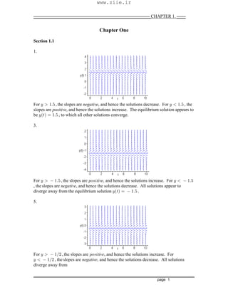
1. —————————————————————————— ——CHAPTER 1.
________________________________________________________________________
page 1
Chapter One
Section 1.1
1.
For , the slopes areC  "Þ& negative, and hence the solutions decrease. For , theC  "Þ&
slopes are , and hence the solutions increase. The equilibrium solution appears topositive
be , to which all other solutions converge.C > œ "Þ&a b
3.
For , the slopes areC   "Þ& :9=3tive, and hence the solutions increase. For C   "Þ&
, the slopes are , and hence the solutions decrease. All solutions appear tonegative
diverge away from the equilibrium solution .C > œ  "Þ&a b
5.
For , the slopes areC   "Î# :9=3tive, and hence the solutions increase. For
C   "Î# , the slopes are , and hence the solutions decrease. All solutionsnegative
diverge away from
www.ziie.ir

2. —————————————————————————— ——CHAPTER 1.
________________________________________________________________________
page 2
the equilibrium solution .C > œ  "Î#a b
6.
For , the slopes areC   # :9=3tive, and hence the solutions increase. For ,C   #
the slopes are , and hence the solutions decrease. All solutions diverge awaynegative
from
the equilibrium solution .C > œ  #a b
8. For solutions to approach the equilibrium solution , we must haveall C > œ #Î$a b
C  ! C  #Î$ C  ! C  #Î$w w
for , and for . The required rates are satisfied by the
differential equation .C œ #  $Cw
9. For solutions than to diverge from , must be another increasingC > œ # C œ # C >a b a b
function for , and a function for . The simplest differentialC  # C  #decreasing
equation
whose solutions satisfy these criteria is .C œ C  #w
10. For solutions than to diverge from , we must haveother C > œ "Î$ C œ "Î$ C  !a b w
for , and for . The required rates are satisfied by the differentialC  "Î$ C  ! C  "Î$w
equation .C œ $C  "w
12.
Note that for and . The two equilibrium solutions are andC œ ! C œ ! C œ & C > œ !w
a b
C > œ & C  ! C  &a b . Based on the direction field, for ; thus solutions with initialw
values than diverge from the solution . For , the slopes aregreater & C > œ & !  C  &a b
negative between, and hence solutions with initial values and all decrease toward the! &
www.ziie.ir

3. —————————————————————————— ——CHAPTER 1.
________________________________________________________________________
page 3
solution . For , the slopes are all ; thus solutions with initialC > œ ! C  !a b positive
values
less than approach the solution .! C > œ !a b
14.
Observe that for and . The two equilibrium solutions areC œ ! C œ ! C œ # C > œ !w
a b
and . Based on the direction field, for ; thus solutions with initialC > œ # C  ! C  #a b w
values than diverge from . For , the slopes are alsogreater # C > œ # !  C  #a b
positive between, and hence solutions with initial values and all increase toward the! #
solution
C > œ # C  !a b . For , the slopes are all ; thus solutions with initialnegative
values than diverge from the solution .less ! C > œ !a b
16. Let be the total amount of the drug in the patient's body ata b a b a b+ Q > in milligrams
any
given time . The drug is administered into the body at a rate of> 2<= &!!a b constant
71Î2<Þ
The rate at which the drug the bloodstream is given by Hence theleaves !Þ%Q > Þa b
accumulation rate of the drug is described by the differential equation
.Q
.>
œ &!!  !Þ% Q 71Î2< Þa b
a b,
Based on the direction field, the amount of drug in the bloodstream approaches the
equilibrium level of "#&! 71 A3>238 + 0/A 29?<= Þa b
18. Following the discussion in the text, the differential equation isa b+
www.ziie.ir

4. —————————————————————————— ——CHAPTER 1.
________________________________________________________________________
page 4
7 œ 71  @
.@
.>
# #
or equivalently,
.@
.> 7
œ 1  @ Þ
# #
a b, ¸ ! ÞAfter a long time, Hence the object attains a given by.@
.> terminal velocity
@ œ Þ
71
_ Ê #
a b- @ œ 71 œ !Þ!%!) 51Î=/- ÞUsing the relation , the required is# #_
#
drag coefficient
a b.
19.
All solutions appear to approach a linear asymptote . It is easy toa bA3>2 =69:/ /;?+6 >9 "
verify that is a solution.C > œ >  $a b
20.
www.ziie.ir

5. —————————————————————————— ——CHAPTER 1.
________________________________________________________________________
page 5
All solutions approach the equilibrium solution C > œ ! Þa b
23.
All solutions appear to from the sinusoid ,diverge C > œ  =38Ð>  Ñ  "a b $
# %È
1
which is also a solution corresponding to the initial value .C ! œ  &Î#a b
25.
All solutions appear to converge to . First, the rate of change is small. TheC > œ !a b
slopes
eventually increase very rapidly in .magnitude
26.
www.ziie.ir

6. —————————————————————————— ——CHAPTER 1.
________________________________________________________________________
page 6
The direction field is rather complicated. Nevertheless, the collection of points at which
the slope field is , is given by the implicit equation The graph ofzero C  'C œ #> Þ$ #
these points is shown below:
The of these curves are at , . It follows that for solutions withy-intercepts C œ ! „ 'È
initial values , all solutions increase without bound. For solutions with initialC  'È
values in the range , the slopes remain , andC   ' !  C  'È Èand negative
hence
these solutions decrease without bound. Solutions with initial conditions in the range
 '  C  !È initially increase. Once the solutions reach the critical value, given by
the equation , the slopes become negative and negative. TheseC  'C œ #>$ #
remain
solutions eventually decrease without bound.
www.ziie.ir

7. —————————————————————————— ——CHAPTER 1.
________________________________________________________________________
page 7
Section 1.2
1 The differential equation can be rewritten asa b+
.C
&  C
œ .> Þ
Integrating both sides of this equation results in , or equivalently, 68 &  C œ >  -k k "
&  C œ - / C ! œ C>
. Applying the initial condition results in the specification ofa b !
the constant as . Hence the solution is- œ &  C C > œ &  C  & / Þ! !a b a b >
All solutions appear to converge to the equilibrium solution C > œ & Þa b
1 Rewrite the differential equation asa b- Þ
.C
"!  #C
œ .> Þ
Integrating both sides of this equation results in , or 68 "!  #C œ >  -"
# "k k
equivalently,
&  C œ - / C ! œ C#>
. Applying the initial condition results in the specification ofa b !
the constant as . Hence the solution is- œ &  C C > œ &  C  & / Þ! !a b a b #>
All solutions appear to converge to the equilibrium solution , but at a rateC > œ &a b faster
than in Problem 1a Þ
2 The differential equation can be rewritten asa b+ Þ
www.ziie.ir

8. —————————————————————————— ——CHAPTER 1.
________________________________________________________________________
page 8
.C
C  &
œ .> Þ
Integrating both sides of this equation results in , or equivalently,68 C  & œ >  -k k "
C  & œ - / C ! œ C>
. Applying the initial condition results in the specification ofa b !
the constant as . Hence the solution is- œ C  & C > œ &  C  & / Þ! !a b a b >
All solutions appear to diverge from the equilibrium solution .C > œ &a b
2 Rewrite the differential equation asa b, Þ
.C
#C  &
œ .> Þ
Integrating both sides of this equation results in , or equivalently,"
# "68 #C  & œ >  -k k
#C  & œ - / C ! œ C#>
. Applying the initial condition results in the specification ofa b !
the constant as . Hence the solution is- œ #C  & C > œ #Þ&  C  #Þ& / Þ! !a b a b #>
All solutions appear to diverge from the equilibrium solution .C > œ #Þ&a b
2 . The differential equation can be rewritten asa b-
.C
#C  "!
œ .> Þ
Integrating both sides of this equation results in , or equivalently,"
# "68 #C  "! œ >  -k k
C  & œ - / C ! œ C#>
. Applying the initial condition results in the specification ofa b !
the constant as . Hence the solution is- œ C  & C > œ &  C  & / Þ! !a b a b #>
www.ziie.ir

9. —————————————————————————— ——CHAPTER 1.
________________________________________________________________________
page 9
All solutions appear to diverge from the equilibrium solution .C > œ &a b
3 . Rewrite the differential equation asa b+
.C
,  +C
œ .> ,
which is valid for . Integrating both sides results in , orC Á , Î+ 68 ,  +C œ >  -
"
"
+ k k
equivalently, . Hence the general solution is,  +C œ - / C > œ ,  - / Î+ Þ+> +>
a b a b
Note that if , then , and is an equilibrium solution.C œ ,Î+ .CÎ.> œ ! C > œ ,Î+a b
a b,
As increases, the equilibrium solution gets closer to , from above.a b a b3 + C > œ !
Furthermore, the convergence rate of all solutions, that is, , also increases.+
As increases, then the equilibrium solutiona b33 , C > œ ,Î+a b also becomes larger. In
this case, the convergence rate remains the same.
If and both increase ,a b a b333 + , but constant,Î+ œ then the equilibrium solution
C > œ ,Î+a b remains the same, but the convergence rate of all solutions increases.
5 . Consider the simpler equation . As in the previous solutions, re-a b+ .C Î.> œ  +C" "
write the equation as
.C
C
œ  + .> Þ
"
"
Integrating both sides results in C > œ - / Þ"a b +>
a b a b a b, Þ C > œ C >  5Now set , and substitute into the original differential equation. We"
find that
www.ziie.ir

10. —————————————————————————— ——CHAPTER 1.
________________________________________________________________________
page 10
 +C  ! œ  + C  5  ," "a b .
That is, , and hence . +5  , œ ! 5 œ ,Î+
a b a b- C > œ - /  ,Î+ Þ. The general solution of the differential equation is This is+>
exactly the form given by Eq. in the text. Invoking an initial condition ,a b a b"( C ! œ C!
the solution may also be expressed as C > œ ,Î+  C  ,Î+ / Þa b a b!
+>
6 . The general solution is , that is, .a b a b a b a b+ : > œ *!!  - / : > œ *!!  :  *!! /> >Î# Î#
!
With , the specific solution becomes . This solution is a: œ )&! : > œ *!!  &!/!
Î#
a b >
decreasing exponential, and hence the time of extinction is equal to the number of
months
it takes, say , for the population to reach . Solving , we find that> *!!  &!/ œ !0
Î#
zero >0
> œ # 68 *!!Î&! œ &Þ()0 a b .months
a b a b a b, : > œ *!!  :  *!! /The solution, , is a exponential as long as!
Î#>
decreasing
:  *!! *!!  :  *!! / œ !! !
Î#
. Hence has only root, given bya b >0
one
> œ # 68 Þ
*!!
*!!  :
0
!
Œ 
a b a b- ,. The answer in part is a general equation relating time of extinction to the value
of
the initial population. Setting , the equation may be written as> œ "#0 months
*!!
*!!  :
œ /
!
'
,
which has solution . Since is the initial population, the appropriate: œ )*(Þ('*" :! !
answer is .: œ )*)! mice
7 . The general solution is . Based on the discussion in the text, time isa b a b+ : > œ : / >!
<>
measured in . Assuming , the hypothesis can be expressed asmonths month days" œ $!
: / œ #: < œ 68 #! !
"<†
. Solving for the rate constant, , with units ofa b per month .
a b, R œ RÎ$!. days months . The hypothesis is stated mathematically as : / œ #:! !
<N/30
.
It follows that , and hence the rate constant is given by<RÎ$! œ 68 # < œ $! 68 # ÎR Þa b a b
The units are understood to be .per month
9 . Assuming , with the positive direction taken as ,a b+ no air resistance downward
Newton's
Second Law can be expressed as
7 œ 71
.@
.>
in which is the measured in appropriate units. The equation can1 gravitational constant
be
www.ziie.ir

11. —————————————————————————— ——CHAPTER 1.
________________________________________________________________________
page 11
written as , with solution The object is released with an.@Î.> œ 1 @ > œ 1>  @ Þa b !
initial
velocity .@!
a b, 2. Suppose that the object is released from a height of above the ground. Usingunits
the
fact that , in which is the of the object, we obtain@ œ .BÎ.> B downward displacement
the
differential equation for the displacement as With the origin placed at.BÎ.> œ 1>  @ Þ!
the point of release, direct integration results in . Based on theB > œ 1> Î#  @ >a b #
!
chosen
coordinate system, the object reaches the ground when . Let be the timeB > œ 2 > œ Xa b
that it takes the object to reach the ground. Then . Using the1X Î#  @ X œ 2#
!
quadratic
formula to solve for ,X
X œ Þ
 @ „ @  #12
1
! !
È
The answer corresponds to the time it takes for the object to fall to the ground.positive
The
negative answer represents a previous instant at which the object could have been
launched
upward , only to ultimately fall downward with speed ,a bwith the same impact speed @!
from a height of above the ground.2 units
a b a b a b- > œ X @ > + Þ. The impact speed is calculated by substituting into in part That is,
@ X œ @  #12a b È ! .
10 , . The general solution of the differential equation is Given thata b a b+ U > œ - / Þb <>
U ! œ "!! - œ "!!a b , the value of the constant is given by . Hence the amount ofmg
thorium-234 present at any time is given by . Furthermore, based on theU > œ "!! /a b <>
hypothesis, setting results in Solving for the rate constant, we> œ " )#Þ!% œ "!! / Þ<
find that or .< œ  68 )#Þ!%Î"!! œ Þ"*(*' < œ Þ!#)#)a b /week /day
a b- X. Let be the time that it takes the isotope to decay to of its originalone-half
amount.
From part , it follows that , in which . Taking thea b+ &! œ "!! / < œ Þ"*(*'<X
/week
natural logarithm of both sides, we find that orX œ $Þ&!"% X œ #%Þ&"weeks s ..+C
11. The general solution of the differential equation is ,.UÎ.> œ  < U U > œ U /a b !
<>
in which is the initial amount of the substance. Let be the time that it takesU œ U !! a b 7
the substance to decay to of its original amount , . Setting in theone-half U > œ! 7
solution,
we have . Taking the natural logarithm of both sides, it follows that!Þ& U œ U /! !
<7
 < œ 68 !Þ& < œ 68 # Þ7 7a b or
www.ziie.ir

12. —————————————————————————— ——CHAPTER 1.
________________________________________________________________________
page 12
12. The differential equation governing the amount of radium-226 is ,.UÎ.> œ  < U
with solution Using the result in Problem 11, and the fact that theU > œ U ! / Þa b a b <>
half-life , the decay rate is given by . The7 œ "'#! < œ 68 # Î"'#!years per yeara b
amount of radium-226, after years, is therefore Let be> U > œ U ! / Þ Xa b a b !Þ!!!%#()'>
the time that it takes the isotope to decay to of its original amount. Then setting$Î%
> œ X,
and , we obtain Solving for the decayU X œ U ! U ! œ U ! / Þa b a b a b a b$ $
% %
!Þ!!!%#()'X
time, it follows that or !Þ!!!%#()' X œ 68 $Î% X œ '(#Þ$'a b years .
13. The solution of the differential equation, with , isU ! œ !a b
U > œ GZ "  / Þa b a b ÎGV>
As , the exponential term vanishes, and hence the limiting value is .> p _ U œ GZP
14 . The rate of the chemical is . At anya b a b+ Ð!Þ!"Ñ $!!accumulation grams per hour
given time , the of the chemical in the pond is> U > Î"!concentration grams per gallona b '
.
Consequently, the chemical the pond at a rate of .leaves grams per houra b a b$ ‚ "! U >%
Hence, the rate of change of the chemical is given by
.U
.>
œ $  !Þ!!!$ U >a b gm/hr .
Since the pond is initially free of the chemical, .U ! œ !a b
a b, . The differential equation can be rewritten as
.U
"!!!!  U
œ !Þ!!!$ .> Þ
Integrating both sides of the equation results in . 68 "!!!!  U œ !Þ!!!$>  Gk k
Taking
the natural logarithm of both sides gives . Since , the"!!!!  U œ - / U ! œ !!Þ!!!$>
a b
value of the constant is . Hence the amount of chemical in the pond at any- œ "!!!!
time
is . Note that . SettingU > œ "!!!! "  / "a b a b!Þ!!!$>
grams year hoursœ )('!
> œ )('! U )('! œ *#((Þ((, the amount of chemical present after is ,one year gramsa b
that is, .*Þ#(((( kilograms
a b- . With the rate now equal to , the governing equation becomesaccumulation zero
.UÎ.> œ  !Þ!!!$ U >a b Resetting the time variable, we now assign the newgm/hr .
initial value as .U ! œ *#((Þ((a b grams
a b a b a b. - U > œ *#((Þ(( / Þ. The solution of the differential equation in Part is !Þ!!!$>
Hence, one year the source is removed, the amount of chemical in the pond isafter
U )('! œ '(!Þ"a b .grams
www.ziie.ir

13. —————————————————————————— ——CHAPTER 1.
________________________________________________________________________
page 13
a b/ >. Letting be the amount of time after the source is removed, we obtain the equation
"! œ *#((Þ(( / Þ  !Þ!!!$ > œ!Þ!!!$>
Taking the natural logarithm of both sides,
œ 68 "!Î*#((Þ(( > œ ##ß ((' œ #Þ'a b or .hours years
a b0
15 . It is assumed that dye is no longer entering the pool. In fact, the rate at which thea b+
dye the pool isleaves kg/min gm per hour#!! † ; > Î'!!!! œ #!! '!Î"!!! ; > Î'!c d a bc da b a b
.
Hence the equation that governs the amount of dye in the pool is
.;
.>
œ  !Þ# ; a bgm/hr .
The initial amount of dye in the pool is .; ! œ &!!!a b grams
a b, . The solution of the governing differential equation, with the specified initial value,
is ; > œ &!!! / Þa b !Þ# >
a b- > œ %. The amount of dye in the pool after four hours is obtained by setting . That is,
; % œ &!!! / œ ##%'Þ'% '!ß !!!a b !Þ)
. Since size of the pool is , thegrams gallons
concentration grams/gallonof the dye is .!Þ!$(%
a b. X. Let be the time that it takes to reduce the concentration level of the dye to
!Þ!# "ß #!!. At that time, the amount of dye in the pool is . Usinggrams/gallon grams
the answer in part , we have . Taking the natural logarithm ofa b, &!!! / œ "#!!!Þ# X
both sides of the equation results in the required time .X œ (Þ"% hours
a b/ !Þ# œ #!!Î"!!!. Note that . Consider the differential equation
.; <
.> "!!!
œ  ; .
Here the parameter corresponds to the , measured in .< flow rate gallons per minute
Using the same initial value, the solution is given by In order; > œ &!!! / Þa b < >Î"!!!
to determine the appropriate flow rate, set and . (Recall that of> œ % ; œ "#!! "#!! gm
www.ziie.ir

14. —————————————————————————— ——CHAPTER 1.
________________________________________________________________________
page 14
dye has a concentration of ). We obtain the equation!Þ!# "#!! œ &!!! / Þgm/gal < Î#&!
Taking the natural logarithm of both sides of the equation results in the required flow rate
< œ $&( .gallons per minute
www.ziie.ir

15. —————————————————————————— ——CHAPTER 1.
________________________________________________________________________
page 15
Section 1.3
1. The differential equation is second order, since the highest derivative in the equation
is of order . The equation is , since the left hand side is a linear function oftwo linear C
and
its derivatives.
3. The differential equation is , since the highest derivative of the functionfourth order C
is of order . The equation is also , since the terms containing the dependentfour linear
variable is linear in and its derivatives.C
4. The differential equation is , since the only derivative is of order . Thefirst order one
dependent variable is , hence the equation is .squared nonlinear
5. The differential equation is . Furthermore, the equation is ,second order nonlinear
since the dependent variable is an argument of the , which is a linearC sine function not
function.
7. . HenceC > œ / Ê C > œ C > œ / C  C œ ! Þ" "" " "a b a b a b> w ww > ww
Also, and . ThusC > œ -9=2 > Ê C > œ =382 > C > œ -9=2 > C  C œ ! Þ# " # #a b a b a bw ww ww
#
9. . Substituting into the differential equation, we haveC > œ $>  > Ê C > œ $  #>a b a b# w
> $  #>  $>  > œ $>  #>  $>  > œ >a b a b# # # #
. Hence the given function is a solution.
10. and Clearly, isC > œ >Î$ Ê C > œ "Î$ C > œ C > œ C > œ ! Þ C >" "" " " "a b a b a b a b a b a bw ww www wwww
a solution. Likewise, , ,C > œ /  >Î$ Ê C > œ  /  "Î$ C > œ /# # #a b a b a b> w > ww >
C > œ  / C > œ /www > wwww >
# #a b a b, . Substituting into the left hand side of the equation, we
find that . Hence both/  %  /  $ /  >Î$ œ /  %/  $/  > œ >> > > > > >
a b a b
functions are solutions of the differential equation.
11. and . Substituting into the leftC > œ > Ê C > œ > Î# C > œ  > Î%"
"Î# "Î# $Î#
" "a b a b a bw ww
hand side of the equation, we have
#>  > Î%  $> > Î#  > œ  > Î#  $ > Î#  >
œ !
#ˆ ‰ ˆ ‰$Î# "Î# "Î# "Î# "Î# "Î#
Likewise, and . Substituting into the leftC > œ > Ê C > œ  > C > œ # >#
" # $
# #a b a b a bw ww
hand side of the differential equation, we have #> # >  $>  >  > œ % > #
a b a b$ # " "
 $ >  > œ !" "
. Hence both functions are solutions of the differential equation.
12. and . Substituting into the left handC > œ > Ê C > œ  #> C > œ ' >"
#
" "
$ %
a b a b a bw ww
side of the differential equation, we have > ' >  &>  #>  % > œ ' > #
a b a b% $ # #
 "! >  % > œ ! C > œ > 68 > Ê C > œ >  #> 68 ># #
#
 $ $
#. Likewise, anda b a b2 w
C > œ  & >  ' > 68 >ww
#
% %
a b . Substituting into the left hand side of the equation, we have
>  & >  ' > 68 >  &> >  #> 68 >  % > 68 > œ  & >  ' > 68 > #
a b a b a b% % $ $   2 2 2
www.ziie.ir

16. —————————————————————————— ——CHAPTER 1.
________________________________________________________________________
page 16
 & >  "! > 68 >  % > 68 > œ ! Þ  2 2 2
Hence both functions are solutions of the
differential equation.
13. andC > œ -9= > 68 -9= >  > =38 > Ê C > œ  =38 > 68 -9= >  > -9= >a b a b a b a bw
C > œ  -9= > 68 -9= >  > =38 >  =/- >ww
a b a b . Substituting into the left hand side of the
differential equation, we have a b a ba b -9= > 68 -9= >  > =38 >  =/- >  -9= > 68 -9= > 
 > =38 > œ  -9= > 68 -9= >  > =38 >  =/- >  -9= > 68 -9= >  > =38 > œ =/- >a b a b .
Hence the function is a solution of the differential equation.C >a b
15. Let . Then , and substitution into the differential equationC > œ / C > œ < /a b a b<> ww # <>
results in . Since , we obtain the algebraic equation< /  # / œ ! / Á ! <  # œ !Þ# <> <> <> #
The roots of this equation are < œ „ 3 # Þ"ß#
È
17. and . Substituting into the differentialC > œ / Ê C > œ < / C > œ < /a b a b a b<> w <> ww # <>
equation, we have . Since , we obtain the algebraic< /  </  ' / œ ! / Á !# <> <> <> <>
equation , that is, . The roots are , .<  <  ' œ ! <  # <  $ œ ! < œ  $ ##
a ba b "ß#
18. Let . Then , and . SubstitutingC > œ / C > œ </ C > œ < / C > œ < /a b a b a b a b<> w <> ww # <> www $ <>
the derivatives into the differential equation, we have . Since< /  $< /  #</ œ !$ <> # <> <>
/ Á ! <  $<  #< œ ! Þ<> $ #
, we obtain the algebraic equation By inspection, it follows
that . Clearly, the roots are , and< <  " <  # œ ! < œ ! < œ " < œ # Þa ba b " # $
20. and . Substituting the derivativesC > œ > Ê C > œ < > C > œ < <  " >a b a b a b a b< w < ww <" #
into the differential equation, we have . After> < <  " >  %> < >  % > œ !# < < <
c d a ba b # "
some algebra, it follows that . For , we obtain the< <  " >  %< >  % > œ ! > Á !a b < < <
algebraic equation The roots of this equation are and<  &<  % œ ! Þ < œ " < œ % Þ#
" #
21. The order of the partial differential equation is , since the highest derivative, intwo
fact each one of the derivatives, is of . The equation is , since the leftsecond order linear
hand side is a linear function of the partial derivatives.
23. The partial differential equation is , since the highest derivative, and infourth order
fact each of the derivatives, is of order . The equation is , since the left handfour linear
side is a linear function of the partial derivatives.
24. The partial differential equation is , since the highest derivative of thesecond order
function is of order . The equation is , due to the product on? Bß C ? † ?a b two nonlinear B
the left hand side of the equation.
25. and? Bß C œ -9= B -9=2 C Ê œ  -9= B -9=2 C œ -9= B -9=2 C Þ"a b ` ? ` ?
`B `C
# #
" "
# #
It is evident that Likewise, given , the second` ? ` ?
`B `C
# ## #
" "
# # œ ! Þ ? Bß C œ 68 B  C#a b a b
derivatives are
www.ziie.ir

17. —————————————————————————— ——CHAPTER 1.
________________________________________________________________________
page 17
` ? # %B
`B B  C
œ 
B  C
` ? # %C
`C B  C
œ 
B  C
# #
# # # # #
# #
# # # # #
2
2
a b
a b
#
#
Adding the partial derivatives,
` ? ` ? # %B # %C
`B `C B  C B  C
 œ   
B  C B  C
œ 
% %
B  C B  C
œ !
# # # #
# # # # # ## # # #
# # # #
2 2
a b a b
a b
# #
# #
#
a bB  C
.
Hence is also a solution of the differential equation.? Bß C#a b
27. Let . Then the second derivatives are? Bß > œ =38 B =38 +>"a b - -
` ?
`B
œ  =38 B =38 +>
` ?
`>
œ  + =38 B =38 +>
#
#
#
#
#
# #
"
"
- - -
- - -
It is easy to see that . Likewise, given , we have+ œ ? Bß > œ =38 B  +>#
#
` ? ` ?
`B `>
# #
# #
" "
a b a b
` ?
`B
œ  =38 B  +>
` ?
`>
œ  + =38 B  +>
#
#
#
#
#
#
#
a b
a b
Clearly, is also a solution of the partial differential equation.? Bß >#a b
28. Given the function , the partial derivatives are? Bß > œ Î> /a b È1 B Î% ># #
!
? œ  
Î> / Î> B /
# > % >
? œ  
> /
#>
B /
% > >
BB
B Î% > # B Î% >
# % #
>
B Î% >
#
# B Î% >
# #
È È
È È
È
1 1
! !
1 1
!
# # # #
# # # #
! !
! !
It follows that .!#
? œ ? œ BB >
# >B /
% > >
È ˆ ‰
È
1 !
!
# # B Î% ># #
# #
!
Hence is a solution of the partial differential equation.? Bß >a b
www.ziie.ir

18. —————————————————————————— ——CHAPTER 1.
________________________________________________________________________
page 18
29 .a b+
a b, Þ The path of the particle is a circle, therefore are intrinsic to thepolar coordinates
problem. The variable is radial distance and the angle is measured from the vertical.< )
Newton's Second Law states that In the direction, the equation of! F aœ 7 Þ tangential
motion may be expressed as , in which the , that is,! J œ 7 +) ) tangential acceleration
the linear acceleration the path is is in the directionalong positive+ œ P . Î.> Þ Ð +) )
# #
)
of increasing . Since the only force acting in the tangential direction is the component) Ñ
of weight, the equation of motion is
 71 =38 œ 7P Þ
.
.>
)
)#
#
ÐNote that the equation of motion in the radial direction will include the tension in the
rod .Ñ
a b- . Rearranging the terms results in the differential equation
. 1
.> P
 =38 œ ! Þ
#
#
)
)
www.ziie.ir

19. —————————————————————————— ——CHAPTER 2.
________________________________________________________________________
page 18
Chapter Two
Section 2.1
1a b+ Þ
a b, Þ Based on the direction field, all solutions seem to converge to a specific increasing
function.
a b a b a b- Þ > œ / C > œ >Î$  "Î*  /  - / ÞThe integrating factor is , and hence. $> #> $>
It follows that all solutions converge to the function C > œ >Î$  "Î* Þ"a b
2a b+ Þ
a b, . All slopes eventually become positive, hence all solutions will increase without
bound.
a b a b a b- Þ > œ / C > œ > / Î$  - / ÞThe integrating factor is , and hence It is. #> $ #> #>
evident that all solutions increase at an exponential rate.
3a b+
www.ziie.ir

20. —————————————————————————— ——CHAPTER 2.
________________________________________________________________________
page 19
a b a b, C > œ " Þ. All solutions seem to converge to the function !
a b a b a b- Þ > œ / C > œ > / Î#  "  - / ÞThe integrating factor is , and hence It is. #> # > >
clear that all solutions converge to the specific solution .C > œ "!a b
4 .a b+
a b, . Based on the direction field, the solutions eventually become oscillatory.
a b a b- Þ > œ >The integrating factor is , and hence the general solution is.
C > œ  =38 #> 
$-9= #> $ -
%> # >
a b a b
a b
in which is an arbitrary constant. As becomes large, all solutions converge to the- >
function C > œ $=38 #> Î# Þ"a b a b
5 .a b+
www.ziie.ir

21. —————————————————————————— ——CHAPTER 2.
________________________________________________________________________
page 20
a b, . All slopes eventually become positive, hence all solutions will increase without
bound.
a b a b a b'- Þ > œ /B:  #.> œ / ÞThe integrating factor is The differential equation. #>
can
be written as , that is, Integration of both/ C  #/ C œ $/ / C œ $/ Þ#> w #> > #> >w
a b
sides of the equation results in the general solution It follows thatC > œ  $/  - / Þa b > #>
all solutions will increase exponentially.
6a b+
a b a b, Þ C > œ ! ÞAll solutions seem to converge to the function !
a b a b- Þ > œ >The integrating factor is , and hence the general solution is. #
C > œ   
-9= > =38 #> -
> > >
a b
a b a b
# #
in which is an arbitrary constant. As becomes large, all solutions converge to the- >
function C > œ ! Þ!a b
7 .a b+
www.ziie.ir

22. —————————————————————————— ——CHAPTER 2.
________________________________________________________________________
page 21
a b a b, Þ C > œ ! ÞAll solutions seem to converge to the function !
a b a b a b a b- Þ > œ /B: > C > œ > /  - / ÞThe integrating factor is , and hence It is. # # > ># #
clear that all solutions converge to the function .C > œ !!a b
8a b+
a b a b, Þ C > œ ! ÞAll solutions seem to converge to the function !
a b a b a b c da b- Þ > œ C > œ >+8 >  G Î ÞSince , the general solution is. a b a b"  > "  ># ## #"
It follows that all solutions converge to the function .C > œ !!a b
9a b+ Þ
www.ziie.ir

23. —————————————————————————— ——CHAPTER 2.
________________________________________________________________________
page 22
a b, . All slopes eventually become positive, hence all solutions will increase without
bound.
a b a b ˆ ‰'- Þ > œ /B: .> œ /The integrating factor is . The differential equation can. "
#
>Î#
be written as , that is, Integration/ C  / CÎ# œ $> / Î# œ $> / Î#Þ>Î# w >Î# >Î# >Î#ˆ ‰/ CÎ#>Î# w
of both sides of the equation results in the general solution AllC > œ $>  '  - / Þa b >Î#
solutions approach the specific solution C > œ $>  ' Þ!a b
10 .a b+
a b, C  !. For , the slopes are all positive, and hence the corresponding solutions
increase
without bound. For , almost all solutions have negative slopes, and hence solutionsC  !
tend to decrease without bound.
a b- Þ >First divide both sides of the equation by . From the resulting , thestandard form
integrating factor is . The differential equation can be.a b ˆ ‰'> œ /B: .> œ "Î> "
>
written as , that is, Integration leads to the generalC Î>  CÎ> œ > / CÎ> œ > / Þw # > >w
a b
solution For , solutionsC > œ  >/  - > Þ - Á !a b >
diverge, as implied by the direction
field. For the case , the specific solution is- œ ! C > œ  >/a b >
, which evidently
approaches as .zero > p _
11 .a b+
a b, Þ The solutions appear to be oscillatory.
www.ziie.ir

24. —————————————————————————— ——CHAPTER 2.
________________________________________________________________________
page 23
a b a b a b a b a b- Þ > œ / C > œ =38 #>  # -9= #>  - / ÞThe integrating factor is , and hence. > >
It is evident that all solutions converge to the specific solution C > œ =38 #>  #!a b a b
-9= #>a b .
12a b+ Þ
a b, . All solutions eventually have positive slopes, and hence increase without bound.
a b a b- Þ > œ /The integrating factor is . The differential equation can be. #>
written as , that is, Integration of both/ C  / CÎ# œ $> Î# / CÎ# œ $> Î#Þ>Î# w >Î# # >Î# #w
ˆ ‰
sides of the equation results in the general solution ItC > œ $>  "#>  #%  - / Þa b # >Î#
follows that all solutions converge to the specific solution .C > œ $>  "#>  #%!a b #
14. The integrating factor is . After multiplying both sides by , the. .a b a b> œ / >#>
equation can be written as Integrating both sides of the equation resultsˆ ‰/ C œ > Þ2> w
in the general solution Invoking the specified condition, weC > œ > / Î#  - / Þa b # #> #>
require that . Hence , and the solution to the initial value/ Î#  - / œ ! - œ  "Î## #
problem is C > œ >  " / Î# Þa b a b# #>
16. The integrating factor is . Multiplying both sides by ,. .a b a bˆ ‰'> œ /B: .> œ > >#
>
#
the equation can be written as Integrating both sides of the equationa b a b> C œ -9= > Þ# w
results in the general solution Substituting and settingC > œ =38 > Î>  - > Þ > œa b a b # #
1
the value equal to zero gives . Hence the specific solution is- œ ! C >a b œ =38 > Î> Þa b #
17. The integrating factor is , and the differential equation can be written as.a b> œ /#>
Integrating, we obtain Invoking the specified initialˆ ‰ a b/ C œ " Þ / C > œ >  - Þ 2 2> >w
condition results in the solution C > œ >  # / Þa b a b #>
19. After writing the equation in standard orm0 , we find that the integrating factor is
. .a b a bˆ ‰'> œ /B: .> œ > >%
>
%
. Multiplying both sides by , the equation can be written as
ˆ ‰ a b a b> C œ > / Þ > C > œ  >  " /  - Þ% > % >w
Integrating both sides results in Letting
> œ  " and setting the value equal to zero gives Hence the specific solution of- œ ! Þ
the initial value problem is C > œ  >  > / Þa b ˆ ‰$ % >
21 .a b+
www.ziie.ir

25. —————————————————————————— ——CHAPTER 2.
________________________________________________________________________
page 24
The solutions appear to diverge from an apparent oscillatory solution. From the
direction
field, the critical value of the initial condition seems to be . For , the+ œ  " +   "!
solutions increase without bound. For , solutions decrease without bound.+   "
a b, Þ The integrating factor is . The general solution of the differential.a b> œ / Î#>
equation is . The solution is sinusoidal as longC > œ )=38 >  %-9= > Î&  - /a b a ba b a b >Î#
as . The- œ ! initial value of this sinusoidal solution is
+ œ! a ba b a b)=38 !  %-9= ! Î& œ  %Î& Þ
a b a b- Þ ,See part .
22a b+ Þ
All solutions appear to eventually initiallyincrease without bound. The solutions
increase
or decrease, depending on the initial value . The critical value seems to be+ + œ  " Þ!
a b, Þ The integrating factor is , and the general solution of the differential.a b> œ / Î#>
equation is Invoking the initial condition , theC > œ  $/  - / Þ C ! œ +a b a b>Î$ >Î#
solution
may also be expressed as Differentiating, follows thatC > œ  $/  +  $ / Þa b a b>Î$ >Î#
C ! œ  "  +  $ Î# œ +  " Î# Þw
a b a b a b The critical value is evidently + œ  " Þ!
www.ziie.ir

26. —————————————————————————— ——CHAPTER 2.
________________________________________________________________________
page 25
a b- + œ  ". For , the solution is! C > œ  $/  # / >a b a b>Î$ >Î#
, which for large is
dominated by the term containing / Þ>Î#
is .C > œ )=38 >  %-9= > Î&  - /a b a ba b a b >Î#
23a b+ Þ
As , solutions increase without bound if , and solutions decrease> p ! C " œ +  Þ%a b
without bound if C " œ +  Þ% Þa b
a b a b ˆ ‰', > œ /B: .> œ > / Þ. The integrating factor is The general solution of the. >"
>
>
differential equation is . Invoking the specified value ,C > œ > /  - / Î> C " œ +a b a b> >
we have . That is, . Hence the solution can also be expressed as"  - œ + / - œ + /  "
C > œ > /  + /  " / Î>a b a b> >
. For small values of , the second term is dominant.>
Setting , critical value of the parameter is+ /  " œ ! + œ "Î/ Þ!
a b- +  "Î/ +  "Î/. For , solutions increase without bound. For , solutions decrease
without bound. When , the solution is+ œ "Î/ C > œ > / ! > p !a b >
, which approaches as
.
24 .a b+
As , solutions increase without bound if , and solutions decrease> p ! C " œ +  Þ%a b
without bound if C " œ +  Þ% Þa b
www.ziie.ir

27. —————————————————————————— ——CHAPTER 2.
________________________________________________________________________
page 26
a b a b a b a b, C œ + C > œ +  -9= > Î>. Given the initial condition, , the solution is Î# Î%1 1#
Þ
Since , solutions increase without bound if , and solutionslim
>Ä
#
!
-9= > œ " +  %Î1
decrease without bound if Hence the critical value is+  %Î Þ1#
+ œ %Î œ !Þ%&#)%(ÞÞÞ! 1#
.
a b a b a b a b- Þ + œ %Î C > œ "  -9= > Î> C > œ "Î#For , the solution is , and . Hence the1#
>Ä
lim
!
solution is bounded.
25. The integrating factor is Therefore general solution is.a b ˆ ‰'> œ /B: .> œ / Þ"
#
>Î#
C > œ %-9= >  )=38 > Î&  - / Þa b c da b a b  Î#>
Invoking the initial condition, the specific
solution is . Differentiating, it follows thatC > œ %-9= >  )=38 >  * / Î&a b c da b a b >Î#
C > œ  %=38 >  )-9= >  %Þ& / Î&
C > œ  %-9= >  )=38 >  #Þ#& / Î&
w >
ww >
a b a b a b ‘
a b a b a b ‘
 Î#
 Î#
Setting , the first solution is , which gives the location of theC > œ ! > œ "Þ$'%$w
a b " first
stationary point. Since . TheC >  !ww
a b" , the first stationary point in a local maximum
coordinates of the point are .a b"Þ$'%$ ß Þ)#!!)
26. The integrating factor is , and the differential equation.a b ˆ ‰'> œ /B: .> œ /#
$
># Î$
can
be written as The general solution isa b a b/ C œ /  > / Î# Þ C > œ# Î$ # Î$ # Î$> > >w
Ð#"  '>ÑÎ) 
 Ð#"  '>ÑÎ)   #"Î)- / C > œ C /# Î$ # Î$
!
> >
. Imposing the initial condition, we have .a b a b
Since the solution is smooth, the desired intersection will be a point of tangency. Taking
the derivative, Setting , the solutionC > œ  $Î%  #C  #"Î% / Î$ Þ C > œ !w > w
a b a b a b!
# Î$
is Substituting into the solution, the respective at the> œ 68 #"  )C Î* Þ" !
$
# c da b value
stationary point is . Setting this result equal toC > œ  68 $  68 #"  )Ca b a b" !
$ * *
# % ) zero,
we obtain the required initial value C œ #"  * / Î) œ  "Þ'%$ Þ!
%Î$
a b
27. The integrating factor is , and the differential equation can be written as.a b> œ />Î4
a b a b/ C œ $ /  # / -9= #> Þ> > >wÎ Î Î4 4 4
The general solution is
C > œ "#  )-9= #>  '%=38 #> Î'&  - / Þa b c da b a b  Î> 4
Invoking the initial condition, , the specific solution isC ! œ !a b
C > œ "#  )-9= #>  '%=38 #>  ()) / Î'& Þa b a b a b ‘ Î> 4
As , the exponential term will decay, and the solution will oscillate about an> p _
average
value amplitudeof , with an of"# )Î '& ÞÈ
www.ziie.ir

28. —————————————————————————— ——CHAPTER 2.
________________________________________________________________________
page 27
29. The integrating factor is , and the differential equation can be written.a b> œ /$ Î#>
as The general solution isa b a b/ C œ $> /  # / Þ C > œ  #>  %Î$  % / $ Î# $ Î#  Î#> > > >w
 - / Þ C > œ  #>  %Î$  % /  C  "'Î$ / Þ$ Î# $ Î#
!
> > >
Imposing the initial condition, a b a b
As , the term containing will the solution. Its> p _ /$ Î#>
dominate sign will determine
the divergence properties. Hence the critical value of the initial condition is
C œ Þ!  "'Î$
The corresponding solution, , will also decrease withoutC > œ  #>  %Î$  % /a b >
bound.
Note on Problems 31-34 :
Let be , and consider the function , in which1 > C > œ C >  1 > C > p _a b a b a b a b a bgiven " "
as . Differentiating, . Letting be a> p _ C > œ C >  1 > +w w w
a b a b a b" constant, it follows
that C >  +C > œ C >  +C >  1 >  +1 > Þw w w
a b a b a b a b a b a b" " Note that the hypothesis on the
function will be satisfied, if . That is, HenceC > C >  +C > œ ! C > œ - / Þ" " ""a b a b a b a bw +>
C > œ - /  1 > C  +C œ 1 >  +1 > Þa b a b a b a b+> w w
, which is a solution of the equation
For convenience, choose .+ œ "
31. Here , and we consider the linear equation The integrating1 > œ $ C  C œ $ Þa b w
factor is , and the differential equation can be written as The.a b a b> œ / / C œ $/ Þ> > >w
general solution is C > œ $  - / Þa b >
33. Consider the linear equation The integrating1 > œ $  > Þ C  C œ  "  $  > Þa b w
factor is , and the differential equation can be written as.a b a b a b> œ / / C œ #  > / Þ> > >w
The general solution is C > œ $  >  - / Þa b >
34. Consider the linear equation The integrating1 > œ %  > Þ C  C œ %  #>  > Þa b # w #
factor is , and the equation can be written as.a b a b a b> œ / / C œ %  #>  > / Þ> > # >w
The general solution is C > œ %  >  - / Þa b # >
www.ziie.ir

29. —————————————————————————— ——CHAPTER 2.
________________________________________________________________________
page 28
Section 2.2
2. For , the differential equation may be written asB Á  " C .C œ .B Þc da bB Î "  B# $
Integrating both sides, with respect to the appropriate variables, we obtain the relation
C Î# œ 68  - Þ C B œ „ 68  - Þ# " #
$ $k k k k"  B "  B$ $That is, a b É
3. The differential equation may be written as Integrating bothC .C œ  =38 B .B Þ#
sides of the equation, with respect to the appropriate variables, we obtain the relation
 C œ -9= B  - Þ G  -9= B C œ " G"
That is, , in which is an arbitrary constant.a b
Solving for the dependent variable, explicitly, .C B œ "Î G  -9= Ba b a b
5. Write the differential equation as , or-9= #C .C œ -9= B .B =/- #C .C œ -9= B .BÞ# # # #
Integrating both sides of the equation, with respect to the appropriate variables, we obtain
the relation >+8 #C œ =38 B -9= B  B  - Þ
7. The differential equation may be written as Integratinga b a bC  / .C œ B  / .B ÞC B
both sides of the equation, with respect to the appropriate variables, we obtain the
relation
C  # / œ B  # /  - Þ# C # B
8. Write the differential equation as Integrating both sides of thea b"  C#
.C œ B .B Þ#
equation, we obtain the relation , that is,C  C Î$ œ B Î$  - $C  C œ B  GÞ$ $ $ $
9 . The differential equation is separable, with Integrationa b a b+ C .C œ "  #B .B Þ#
yields Substituting and , we find that C œ B  B  - Þ B œ ! C œ  "Î' - œ ' Þ" #
Hence the specific solution is . The isC œ B  B  '" #
explicit form
C B œ "Î Þa b a bB  B  '#
a b,
a b a ba b- B  B  ' œ B  # B  $. Note that . Hence the solution becomes#
singular at
B œ  # B œ $ Þand
10a b a b È+ Þ C B œ  #B  #B  % Þ#
www.ziie.ir

30. —————————————————————————— ——CHAPTER 2.
________________________________________________________________________
page 29
10a b, Þ
11 Rewrite the differential equation as Integrating both sidesa b+ Þ B / .B œ  C .C ÞB
of the equation results in Invoking the initial condition, weB /  / œ  C Î#  - ÞB B #
obtain Hence- œ  "Î# Þ C œ #/  #B /  "Þ# B B
The of the solution isexplicit form
C B œ Þa b È#/  #B /  " C ! œ "ÞB B The positive sign is chosen, since a b
a b, Þ
a b- Þ B œ  "Þ( B œ !Þ(' ÞThe function under the radical becomes near andnegative
11 Write the differential equation as Integrating both sides of thea b+ Þ < .< œ . Þ# "
) )
equation results in the relation Imposing the condition , we < œ 68  - Þ < " œ #"
) a b
obtain .- œ  "Î# The of the solution isexplicit form < œ #Î "  # 68 Þa b a b) )
www.ziie.ir

31. —————————————————————————— ——CHAPTER 2.
________________________________________________________________________
page 30
a b, Þ
a b- Þ  ! ÞClearly, the solution makes sense only if Furthermore, the solution becomes)
singular when , that is,68 œ "Î# œ / Þ) ) È
13a b a b a bÈ+ Þ C B œ  # 68 "  B  % Þ#
a b, Þ
14 . Write the differential equation as Integrating botha b a b+ C .C œ B "  B .B Þ$ "Î##
sides of the equation, with respect to the appropriate variables, we obtain the relation
 C Î# œ "  B  - Þ - œ  $Î# Þ# È # Imposing the initial condition, we obtain
Hence the specific solution can be expressed as TheC œ $  # "  B Þ# È # explicit
form positiveof the solution is TheC B œ "Î $  # "  B Þa b É È # sign is chosen to
satisfy the initial condition.
www.ziie.ir

32. —————————————————————————— ——CHAPTER 2.
________________________________________________________________________
page 31
a b, Þ
a b- Þ The solution becomes singular when # "  B œ $ B œ „ & Î# ÞÈ È# . That is, at
15a b a b È+ Þ C B œ  "Î#  B  "&Î% Þ#
a b, Þ
16 .a b+ Rewrite the differential equation as Integrating both%C .C œ B B  " .B Þ$ #
a b
sides
of the equation results in Imposing the initial condition, we obtainC œ Î%  - Þ%
a bB  "# #
- œ ! Þ  %C œ ! ÞHence the solution may be expressed as The forma bB  "# # %
explicit
of the solution is The is chosen based onC B œ  Þ C ! œ Þa b a bÈa b ÈB  " Î#  "Î ## sign
www.ziie.ir

33. —————————————————————————— ——CHAPTER 2.
________________________________________________________________________
page 32
a b, Þ
a b- Þ B −The solution is valid for all .‘
17a b a b È+ Þ C B œ  &Î#  B  /  "$Î% Þ$ B
a b, Þ
a b- B   "Þ%& Þ. The solution is valid for This value is found by estimating the root of
%B  %/  "$ œ ! Þ$ B
18 . Write the differential equation as Integrating botha b a b a b+ $  %C .C œ /  / .B ÞB B
sides of the equation, with respect to the appropriate variables, we obtain the relation
$C  #C œ  /  /  - Þ C ! œ "# B B
a b a bImposing the initial condition, , we obtain
- œ (Þ $C  #C œ  /  /  (ÞThus, the solution can be expressed as Now by# B B
a b
completing the square on the left hand side, # C  $Î% œa b#
 /  /  '&Î)a bB B
.
Hence the explicit form of the solution is C B œ  $Î%  '&Î"'  -9=2 B Þa b È
www.ziie.ir

34. —————————————————————————— ——CHAPTER 2.
________________________________________________________________________
page 33
a b, Þ
a b k k- '&  "' -9=2 B ! B  #Þ" Þ. Note the , as long as Hence the solution is valid on
the interval . #Þ"  B  #Þ"
19a b+ Þ C B œ  Î$  =38 $ -9= B Þa b a b1 "
$
" #
a b, Þ
20a b+ Þ Rewrite the differential equation as IntegratingC .C œ +<-=38 BÎ "  B .B Þ# #È
both sides of the equation results in Imposing the conditionC Î$ œ +<-=38 B Î#  - Þ$
a b
#
C ! œ ! - œ !Þa b , we obtain formThe of the solution isexplicit C B œ Þa b a bÉ$ $
# +<-=38 B
#Î$
www.ziie.ir

35. —————————————————————————— ——CHAPTER 2.
________________________________________________________________________
page 34
a b, .
a b-  " Ÿ B Ÿ " Þ. Evidently, the solution is defined for
22. The differential equation can be written as Integrating botha b$C  % .C œ $B .B Þ# #
sides, we obtain Imposing the initial condition, the specific solutionC  %C œ B  - Þ$ $
is Referring back to the differential equation, we find that asC  %C œ B  " Þ C p _$ $ w
C p „#Î $ Þ B œ  "Þ#(' "Þ&*) ÞÈ The respective values of the abscissas are ,
Hence the solution is valid for  "Þ#('  B  "Þ&*) Þ
24. Write the differential equation as Integrating both sides,a b a b$  #C .C œ #  / .B ÞB
we obtain Based on the specified initial condition, the solution$C  C œ #B  /  - Þ# B
can be written as , it follows that$C  C œ #B  /  " Þ# B
Completing the square
C B œ  $Î#  #B  /  "$Î% Þ #B  /  "$Î% !a b È B B
The solution is defined if ,
that is, . In that interval, , for It can "Þ& Ÿ B Ÿ # C œ ! B œ 68 # Þa bapproximately w
be verified that . In fact, on the interval of definition. HenceC 68 #  ! C B  !ww ww
a b a b
the solution attains a global maximum at B œ 68 # Þ
26. The differential equation can be written as Integratinga b"  C# "
.C œ # "  B .B Þa b
both sides of the equation, we obtain Imposing the given+<->+8C œ #B  B  - Þ#
initial
condition, the specific solution is Therefore,+<->+8C œ #B  B Þ C B œ >+8 Þ#
a b a b#B  B#
Observe that the solution is defined as long as It is easy to Î#  #B  B  Î# Þ1 1#
see that Furthermore, for and Hence#B  B  "Þ #B  B œ Î# B œ  #Þ' !Þ' Þ# #
1
the solution is valid on the interval Referring back to the differential #Þ'  B  !Þ' Þ
www.ziie.ir

36. —————————————————————————— ——CHAPTER 2.
________________________________________________________________________
page 35
equation, the solution is at Since on the entire intervalstationary B œ  "Þ C B  !ww
a b
of
definition, the solution attains a global minimum at B œ  " Þ
28 . Write the differential equation as Integratinga b a b a b+ C %  C .C œ > "  > .> Þ" " "
both sides of the equation, we obtain Taking68 C  68 C  % œ %>  %68 "  >  - Þk k k k k k
the of both sides, it follows that It followsexponential k k a ba bCÎ C  % œ G / Î "  > Þ%> %
that as , . That is,> p _ CÎ C  % œ "  %Î C  % p _ C > p % Þk k k k a ba b a b
a b a b, Þ C ! œ # G œ "Setting , we obtain that . Based on the initial condition, the solution
may be expressed as Note that , for allCÎ C  % œ  / Î "  > Þ CÎ C  %  !a b a b a b%> %
> !Þ C  % > !ÞHence for all Referring back to the differential equation, it follows
that is always . This means that the solution is . We findCw
positive monotone increasing
that the root of the equation is near/ Î "  > œ $** > œ #Þ)%% Þ%>
a b%
a b a b- Þ C > œ %Note the is an equilibrium solution. Examining the local direction field,
we see that if , then the corresponding solutions converge to . ReferringC !  ! C œ %a b
back to part , we have , for Settinga b a b c d a ba b+ CÎ C  % œ C Î C  % / Î "  > C Á % Þ! ! !
%%>
> œ # C Î C  % œ $Î/ C # Î C #  % Þ, we obtain Now since the function! !a b a b a b a ba b# %
0 C œ CÎ C  % C  % C  %a b a b is for and , we need only solve the equationsmonotone
C Î C  % œ C Î C  % œ Þ! ! ! !
# #% %
a b a b $** $Î/ %!" $Î/a b a band The respective solutions
are andC œ $Þ''## C œ %Þ%!%# Þ! !
30a b0 Þ
www.ziie.ir

37. —————————————————————————— ——CHAPTER 2.
________________________________________________________________________
page 36
31a b-
32 . Observe that Hence the differential equationa b a b ˆ ‰+ B  $C Î#BC œ  Þ# # " $
# B # B
C C"
is .homogeneous
a b a b, C œ B @ @  B @ œ B  $B @ Î#B @. The substitution results in . Thew # # # #
transformed equation is This equation is , with general@ œ "  @ Î#B@ Þw #
a b separable
solution In terms of the original dependent variable, the solution is@  " œ - B Þ#
B  C œ - B Þ# # $
a b- Þ
33a b- Þ
www.ziie.ir

38. —————————————————————————— ——CHAPTER 2.
________________________________________________________________________
page 37
34 Observe that Hence thea b a b  ‘+ Þ %B  $C ÎÐ#B  CÑ œ  #  #  Þ
C C
B B
"
differential equation is .homogeneous
a b a b, C œ B @ @  B @ œ  #  @Î #  @. The substitution results in . The transformedw
equation is This equation is , with general@ œ  @  &@  % ÎÐ#  @ÑB Þw #
a b separable
solution In terms of the original dependent variable, the solutiona b k k@% @" œ GÎB Þ# $
is a b k k%B  C BC œ GÞ#
a b- Þ
35 .a b-
36 Divide by to see that the equation is homogeneous. Substituting , wea b+ Þ B C œ B @#
obtain The resulting differential equation is separable.B @ œ "  @ Þw #
a b
a b a b, Þ "  @ .@ œ B .B ÞWrite the equation as Integrating both sides of the equation, "#
we obtain the general solution In terms of the original "Î "  @ œ 68 B  - Þa b k k
dependent variable, the solution is C œ B G  68 B  B Þc dk k "
www.ziie.ir

39. —————————————————————————— ——CHAPTER 2.
________________________________________________________________________
page 38
a b- Þ
37 The differential equation can be expressed as . Hence thea b ˆ ‰+ Þ C œ w " $
# B # B
C C"
equation is homogeneous. The substitution results in .C œ B @ B @ œ "  &@ Î#@w #
a b
Separating variables, we have #@ "
"&@ B# .@ œ .B Þ
a b, Þ Integrating both sides of the transformed equation yields "
&
68 œ 68 B  -k k"  &@#
k k ,
that is, In terms of the original dependent variable, the general"  &@ œ GÎ B Þ# &
k k
solution is &C œ B  GÎ B Þ# # $
k k
a b- Þ
38 The differential equation can be expressed as . Hence thea b ˆ ‰+ Þ C œ w $ "
# B # B
C C "
equation is homogeneous. The substitution results in , thatC œ B @ B @ œ @  " Î#@w #
a b
is, #@ "
@ " B# .@ œ .B Þ
a b k k, Þ 68 œ 68 B  -Integrating both sides of the transformed equation yields ,k k@  "#
that is, In terms of the original dependent variable, the general solution@  " œ G B Þ#
k k
is C œ G B B  B Þ# # #
k k
www.ziie.ir

40. —————————————————————————— ——CHAPTER 2.
________________________________________________________________________
page 39
a b- Þ
www.ziie.ir

41. —————————————————————————— ——CHAPTER 2.
________________________________________________________________________
page 40
Section 2.3
5 . Let be the amount of salt in the tank. Salt enters the tank of water at a rate ofa b+ U
# "  =38 > œ  =38 > Þ # UÎ"!! Þ" " " "
% # # %
ˆ ‰ It leaves the tank at a rate of9DÎ738 9DÎ738
Hence the differential equation governing the amount of salt at any time is
.U " "
.> # %
œ  =38 >  UÎ&! Þ
The initial amount of salt is The governing ODE isU œ &! 9D Þ! linear, with integrating
factor Write the equation as The.a b ˆ ‰ ˆ ‰> œ / Þ / U œ / Þ>Î&! >Î&! >Î&!w " "
# % =38 >
specific solution is U > œ #&  "#Þ&=38 >  '#&-9= >  '$"&! / Î#&!" 9D Þa b  ‘>Î&!
a b, Þ
a b- Þ The amount of salt approaches a , which is an oscillation of amplitudesteady state
"Î% #& 9D Þabout a level of
6 . The equation governing the value of the investment is . The value ofa b+ .WÎ.> œ < W
the investment, at any time, is given by Setting , the requiredW > œ W / Þ W X œ #Wa b a b! !
<>
time is X œ 68 # Î< Þa b
a b, Þ < œ ( œ Þ!( X ¸ *Þ* C<= ÞFor the case ,%
a b a b a b- Þ + < œ 68 # ÎX X œ )Referring to Part , . Setting , the required interest rate is to
be approximately < œ )Þ'' Þ%
8 . Based on the solution in , with , the value of the investmentsa b a b+ "' W œ !Eq. with!
contributions is given by After years, person A hasW > œ #&ß !!! /  " Þa b a b<>
ten
W œ #&ß !!! "Þ##' œ $!ß '%! Þ $&E $ $a b Beginning at age , the investments can now be
analyzed using the equations andW œ $!ß '%! / W œ #&ß !!! /  " ÞE F
Þ!)> Þ!)>
a b
After years, the balances are andthirty $ $W œ $$(ß ($% W œ #&!ß &(*ÞE F
a b, Þ < W œ $!ß '%! /For an rate , the balances after years are andunspecified thirty E
$!<
W œ #&ß !!! /  " ÞF a b$!<
www.ziie.ir

42. —————————————————————————— ——CHAPTER 2.
________________________________________________________________________
page 41
a b- .
a b. Þ The two balances can be equal.never
11 . Let be the value of the mortgage. The debt accumulates at a rate of , ina b+ W <W
which is the interest rate. Monthly payments of are equivalent to< œ Þ!* )!!annual $
$ per year The differential equation governing the value of the mortgage is*ß '!! Þ
.WÎ.> œ Þ!* W  *ß '!! Þ WGiven that is the original amount borrowed, the debt is!
W > œ W /  "!'ß ''( /  " Þ W $! œ !a b a b a b!
Þ!*> Þ!*>
Setting , it follows that
W œ **ß &!!! $ .
a b, Þ $! #))ß !!!The payment, over years, becomes . The interest paid on thistotal $
purchase is .$ "))ß &!!
13 . The balance at a rate of , and at a constant rate ofa b+ < W 5increases $/yr decreases
$ per year. Hence the balance is modeled by the differential equation ..WÎ.> œ <W  5
The balance at any time is given by W > œ W /  /  " Þa b a b!
<> <>5
<
a b a b, W > œ ÐW  Ñ/  Þ. The solution may also be expressed as Note that if the!
5 5
< <
<>
withdrawal rate is , the balance will remain at a constant level5 œ < W W Þ! ! !
a b a b ’ “- 5  5 W X œ ! X œ 68 Þ. Assuming that , for! ! !
" 5
< 55!
a b. < œ Þ!) 5 œ #5 X œ )Þ''. If and , then! ! years .
a b a b a b/ W > œ ! / , / œ Þ > œ X. Setting and solving for in Part , Now setting<> <> 5
5<W!
results in 5 œ <W / Î /  " Þ!
X X< <
a b
a b a b0 Þ / 5 œ "#ß !!! < œ Þ!) X œ #!In part , let , , and . The required investment
becomes .W œ ""*ß ("&! $
14 Let The general solution is Based on thea b a b+ Þ U œ  < U Þ U > œ U / Þw <>
!
definition of , consider the equation It follows thathalf-life U Î# œ U / Þ! !
&($! <
www.ziie.ir

43. —————————————————————————— ——CHAPTER 2.
________________________________________________________________________
page 42
 &($! < œ 68Ð"Î#Ñ < œ "Þ#!*( ‚ "!, that is, %
per year.
a b a b, U > œ U / Þ. Hence the amount of carbon-14 is given by !
"Þ#!*(‚"! >%
a b a b- Þ U X œ U Î& "Î& œ / ÞGiven that , we have the equation Solving for!
"Þ#!*(‚"! X%
the , the apparent age of the remains is approximatelydecay time years .X œ "$ß $!%Þ'&
15. Let be the population of mosquitoes at any time . The rate of of theT > >a b increase
mosquito population is The population by . Hence the<TÞ #!ß !!!decreases per day
equation that models the population is given by . Note that the.TÎ.> œ <T  #!ß !!!
variable represents . The solution is In the> T > œ T /  /  " Þdays a b a b!
<> <>#!ß!!!
<
absence of predators, the governing equation is , with solution.T Î.> œ <T" "
T > œ T / Þ T ( œ #T #T œ T / Þ" ! " ! ! !a b a b<> (<
Based on the data, set , that is, The growth
rate is determined as Therefore the population,< œ 68 # Î( œ Þ!**!# Þa b per day
including the by birds, ispredation T > œ # ‚ "! /  #!"ß **( /  " œa b a b& Þ!**> Þ!**>
œ #!"ß **(Þ$  "*((Þ$ / ÞÞ!**>
16 . The isa b a b c d+ C > œ /B: #Î"!  >Î"!  #-9=Ð>ÑÎ"! Þ ¸ #Þ*'$# Þdoubling-time 7
a b a b a b, Þ .CÎ.> œ CÎ"! C > œ C ! / ÞThe differential equation is , with solution The>Î"!
doubling-time is given by 7 œ "!68 # ¸ 'Þ*$"& Þa b
a b a b- .CÎ.> œ !Þ&  =38Ð# >Ñ CÎ& Þ. Consider the differential equation The equation is1
separable, with Integrating both sides, with respect to the" "
C &.C œ !Þ"  =38Ð# >Ñ .> Þˆ ‰1
appropriate variable, we obtain Invoking the initial68 C œ >  -9=Ð# >Ñ Î"!  - Þa b1 1 1
condition, the solution is The isC > œ /B: "  >  -9=Ð# >Ñ Î"! Þa b c da b1 1 1 doubling-time
7 ¸ 'Þ$)!% Þ ,The approaches the value found in part .doubling-time a b
a b. .
17 . The differential equation is , with integrating factora b a b+ .CÎ.> œ < > C  5 linear
. . .a b a b a b a b ‘'> œ /B: < > .> Þ C œ  5 > Þ Write the equation as Integration of bothw
www.ziie.ir

44. —————————————————————————— ——CHAPTER 2.
________________________________________________________________________
page 43
sides yields the general solution . In this problem,C œ  5 .  C ! Î > ‘' a b a b a b. 7 7 . .!
the
integrating factor is .a b c da b> œ /B: -9= >  > Î& Þ
a b a b, Þ C > œ ! > œ >The population becomes , if , for some . Referring toextinct ‡ ‡
part ,a b+
we find that C > œ ! Êa b‡
( c da b
!
>
"Î&
-
‡
/B: -9=  Î& . œ & / C Þ7 7 7
It can be shown that the integral on the left hand side increases , frommonotonically zero
to a limiting value of approximately . Hence extinction can happen&Þ!)*$ only if
& / C  &Þ!)*$ C  !Þ)$$$ Þ"Î&
- -, that is,
a b a b a b- , C > œ ! Ê. Repeating the argument in part , it follows that ‡
( c da b
!
>
"Î&
-
‡
/B: -9=  Î& . œ / C Þ
"
5
7 7 7
Hence extinction can happen , that is,only if / C Î5  &Þ!)*$ C  %Þ"''( 5 Þ"Î&
- -
a b. C 5. Evidently, is a function of the parameter .- linear
19 . Let be the of carbon monoxide in the room. The rate of ofa b a b+ U > volume increase
CO CO leaves the roomis The amount of at a rate ofa ba bÞ!% !Þ" œ !Þ!!% 0> Î738 Þ$
a b a b a b!Þ" U > Î"#!! œ U > Î"#!!! 0> Î738 Þ Hence the total rate of change is given by$
the differential equation This equation is and.UÎ.> œ !Þ!!%  U > Î"#!!! Þa b linear
separable, with solution Note thatU > œ %)  %) /B:  >Î"#!!! U œ !a b a b 0> Þ 0> Þ$ $
!
Hence the at any time is given by .concentration %B > œ U > Î"#!! œ U > Î"#a b a b a b
a b a b a b, B > œ %  %/B:  >Î"#!!!. The of in the room is A levelconcentration CO %Þ
of corresponds to . Setting , the solution of the equation!Þ!!!"# !Þ!"# B œ !Þ!"#% a b7
%  %/B:  >Î"#!!! œ !Þ!"# ¸ $'a b is .7 minutes
www.ziie.ir

45. —————————————————————————— ——CHAPTER 2.
________________________________________________________________________
page 44
20 The concentration is It is easy to seea b a b a b+ Þ - > œ 5  TÎ<  -  5  TÎ< / Þ!
<>ÎZ
that - >p_ œ 5  TÎ< Þa b
a b a b, Þ - > œ - / X œ 68Ð#ÑZ Î< X œ 68Ð"!ÑZ Î<Þ. The are and! &! "!
<>ÎZ
reduction times
a b a ba b- Þ X œ 68 "! '&Þ# Î"#ß #!! œ %$!Þ)&The , in , arereduction times years W
X œ 68 "! "&) Î%ß *!! œ ("Þ% à X œ 68 "! "(& Î%'! œ 'Þ!&Q Ia ba b a ba b
X œ 68 "! #!* Î"'ß !!! œ "(Þ'$ ÞS a ba b
21a b- Þ
22 . The differential equation for the motion is Given thea b+ 7 .@Î.> œ  @Î$!  71 Þ
initial condition , the solution is .@ ! œ #! @ > œ  %%Þ"  '%Þ" /B:  >Î%Þ&a b a b a bm/s
Setting , the ball reaches the maximum height at . Integrating@ > œ ! > œ "Þ')$a b" " sec
@ > B > œ $")Þ%&  %%Þ" >  #))Þ%& /B:  >Î%Þ& Þa b a b a b, the position is given by Hence
the is .maximum height mB > œ %&Þ()a b"
a b a b, Þ B > œ ! > œ &Þ"#)Setting , the ball hits the ground at .# # sec
a b- Þ
23 The differential equation for the motion is ,a b+ Þ 7 .@Î.> œ  @  71upward . #
in which . This equation is , with Integrating. œ "Î"$#& .@ œ  .> Þseparable 7
@ 71. #
www.ziie.ir

46. —————————————————————————— ——CHAPTER 2.
________________________________________________________________________
page 45
both sides and invoking the initial condition, Setting@ > œ %%Þ"$$ >+8 Þ%#&  Þ### > Þa b a b
@ > œ ! > œ "Þ*"' @ >a b a b" ", the ball reaches the maximum height at . Integrating , thesec
position is given by Therefore theB > œ "*)Þ(& 68 -9= !Þ### >  !Þ%#&  %)Þ&( Þa b c da b
maximum height mis .B > œ %)Þ&'a b"
a b, Þ 7 .@Î.> œ  @  71 ÞThe differential equation for the motion isdownward . #
This equation is also separable, with For convenience, set at7
71 @. # .@ œ  .> Þ > œ !
the of the trajectory. The new initial condition becomes . Integrating bothtop @ ! œ !a b
sides and invoking the initial condition, we obtain 68 %%Þ"$  @ Î %%Þ"$  @ œ >Î#Þ#&c da b a b
Þ
Solving for the velocity, Integrating , the@ > œ %%Þ"$ "  / Î "  / Þ @ >a b a b a b a b> >Î#Þ#& Î#Þ#&
position is given by To estimate theB > œ **Þ#* 68 / Î "  /  ")'Þ# Þa b a b’ “> > #Î#Þ#& Î#Þ#&
duration secof the downward motion, set , resulting in . Hence theB > œ ! > œ $Þ#('a b# #
total time secthat the ball remains in the air is .>  > œ &Þ"*#1 #
a b- Þ
24 Measure the positive direction of motion . Based on Newton'sa b+ Þ #downward nd
law,
the equation of motion is given by
7 œ Þ
.@
.>
 !Þ(& @  71 !  >  "!
 "# @  71 >  "!œ
,
,
Note that gravity acts in the direction, and the drag force is . During thepositive resistive
first ten seconds of fall, the initial value problem is , with initial.@Î.> œ  @Î(Þ&  $#
velocity This differential equation is separable and linear, with solution@ ! œ ! Þa b fps
@ > œ #%! "  / @ "! œ "('Þ( Þa b a b a b>Î(Þ&
. Hence fps
a b a b, B > œ !. Integrating the velocity, with , the distance fallen is given by
B > œ #%! >  ")!! /  ")!!a b >Î(Þ&
.
Hence .B "! œ "!(%Þ&a b ft
www.ziie.ir

47. —————————————————————————— ——CHAPTER 2.
________________________________________________________________________
page 46
a b- Þ > œ !For computational purposes, reset time to . For the remainder of the motion,
the initial value problem is , with specified initial velocity.@Î.> œ  $#@Î"&  $#
@ ! œ "('Þ( Þ @ > œ "&  "'"Þ( / Þ > p _a b a bThe solution is given by As ,fps $# >Î"&
@ > p @ œ "& Þ B ! œ "!(%Þ&a b a bP Integrating the velocity, with , the distance fallenfps
after the parachute is open is given by To find theB > œ "& >  (&Þ) /  ""&!Þ$ Þa b $# >Î"&
duration of the second part of the motion, estimate the root of the transcendental equation
"& X  (&Þ) /  ""&!Þ$ œ &!!! Þ X œ #&'Þ' Þ$# XÎ"&
The result is sec
a b. Þ
25 . Measure the positive direction of motion . The equation of motion isa b+ upward
given by . The initial value problem is ,7.@Î.> œ  5 @  71 .@Î.> œ  5@Î7  1
with . The solution is Setting@ ! œ @ @ > œ  71Î5  @  71Î5 / Þa b a b a b! !
5>Î7
@ > œ ! > œ 7Î5 68 71  5 @ Î71 Þa b a b c da b7 7, the maximum height is reached at time !
Integrating the velocity, the position of the body is
B > œ  71 >Î5  1  Ð"  / ÑÞ
7 7 @
5 5
a b ” •Š ‹
#
5>Î7!
Hence the maximum height reached is
B œ B > œ  1 68 Þ
7 @ 7 71  5 @
5 5 71
7 7
! !
a b Š ‹ ” •
#
a b a b, Þ ¥ " 68 "  œ     áRecall that for ,$ $ $ $ $ $" " "
# $ %
# $ %
26 .a b a b, œ  5 @  71 / œ  1> Þlim lim
5Ä ! 5Ä !
71 5 @ 71 /
5 7
> 5>Î7a b!
5>Î7
!
a b  ‘ˆ ‰- Þ   @ / œ ! / œ ! Þ, sincelim lim
7 Ä ! 7 Ä !
71 71
5 5
5>Î7 5>Î7
!
28 . In terms of displacement, the differential equation isa b+ 7@ .@Î.B œ  5 @  71 Þ
This follows from the : . The differential equation ischain rule .@ .@ .B .@
.> .B .> .>œ œ @
separable, with
www.ziie.ir

48. —————————————————————————— ——CHAPTER 2.
________________________________________________________________________
page 47
B @ œ   68 Þ
7@ 7 1 71  5 @
5 5 71
a b º º
#
#
The inverse , since both and are monotone increasing. In terms of the givenexists B @
parameters, B @ œ  "Þ#& @  "&Þ$" 68 !Þ!)"' @  " Þa b k k
a b a b, Þ B "! œ "$Þ%& 5 œ !Þ#%. The required value is .meters
a b a b- Þ + @ œ "! B œ "!In part , set and .m/s meters
29 Let represent the height above the earth's surface. The equation of motion isa b+ Þ B
given by , in which is the universal gravitational constant. The7 œ  K K.@ Q7
.> VBa b#
symbols and are the and of the earth, respectively. By the chain rule,Q V mass radius
7@ œ  K
.@ Q7
.B V  Ba b# .
This equation is separable, with Integrating both sides,@ .@ œ  KQ V  B .B Þa b#
and
invoking the initial condition , the solution is@ ! œ #1V @ œ #KQ V  B a b a bÈ # "
 #1V  #KQÎV Þ 1 œ KQÎVFrom elementary physics, it follows that . Therefore#
@ B œ #1 VÎ V  B Þa b a bÈ ’ “È Note that mi/hr .1 œ ()ß &%& #
a b È ’ “È, Þ .BÎ.> œ #1 VÎ V  BWe now consider . This equation is also separable,
with By definition of the variable , the initial condition isÈ ÈV  B .B œ #1 V .> Þ B
B ! œ !Þ B > œ #1 V >  V  V Þa b a b  ‘ˆ ‰ÈIntegrating both sides, we obtain $ #
# $
$Î# #Î$
Setting the distance , and solving for , the duration of such aB X  V œ #%!ß !!! Xa b
flight would be X ¸ %* hours .
32 Both equations are linear and separable. The initial conditions area b a b+ Þ @ ! œ ? -9=
E
and . The two solutions are andA ! œ ? =38 E @ > œ ? -9= E / A > œ  1Î< a b a b a b<>
 ? =38 E  1Î< / Þa b <>
www.ziie.ir

49. —————————————————————————— ——CHAPTER 2.
________________________________________________________________________
page 48
a b a b, Þ +Integrating the solutions in part , and invoking the initial conditions, the
coordinates are andB > œ -9= E "  /a b a b?
<
<>
C > œ  1>Î<  1  ?< =38 E  2< Î<  =38 E  1Î< / Þ
?
<
a b ˆ ‰ Š ‹# # # <>
a b- Þ
a b. Þ X $&!Let be the time that it takes the ball to go horizontally. Then from above,ft
/ œ ? -9= E  (! Î? -9= E ÞXÎ&
a b At the same time, the height of the ball is given by
C X œ  "'! X  #'(  "#&?=38 E  Ð)!!  &? =38 EÑ ? -9= E  (! Î? -9= E Þa b c da b
Hence and must satisfy the inequalityE ?
)!!68  #'(  "#&?=38 E  Ð)!!  &? =38 EÑ ? -9= E  (! Î? -9= E "! Þ
? -9= E  (!
? -9= E
” • c da b
33 Solving equation , . The answer isa b a b a b c da b+ Þ 3 C B œ 5  C ÎCw # "Î#
positive
chosen, since is an function of .C Bincreasing
a b, C œ 5 =38 > .C œ #5 =38 > -9= > .> Þ. Let . Then Substituting into the equation in# # #
part , we find thata b+
#5 =38 > -9= > .> -9= >
.B =38 >
œ Þ
#
Hence #5 =38 > .> œ .B Þ# #
a b- Þ œ #> 5 =38 . œ .B ÞLetting , we further obtain Integrating both sides of the) )# #
#
)
equation and noting that corresponds to the , we obtain the solutions> œ œ !) origin
B œ 5  =38 Î# , C œ 5 "  -9= Î# Þa b a b c d a b a ba b) ) ) ) )# #
and from part
a b a b a b. CÎB œ "  -9= Î  =38 Þ B œ " C œ #. Note that Setting , , the solution of) ) )
the equation is . Substitution into either of thea b a b"  -9= Î  =38 œ # ¸ "Þ%!") ) ) )
expressions yields 5 ¸ #Þ"*$ Þ
www.ziie.ir

50. —————————————————————————— ——CHAPTER 2.
________________________________________________________________________
page 49
Section 2.4
2. Considering the roots of the coefficient of the leading term, the ODE has unique
solutions on intervals not containing or . Since , the initial value problem! % # − ! ß %a b
has a unique solution on the interval a b! ß % Þ
3. The function is discontinuous at of . Since , the>+8 >  odd multiples 1 1 1
# # #
$
1
initial value problem has a unique solution on the interval ˆ ‰1 1
# #
$
ß Þ
5. and . These functions are discontinuous at: > œ #>Î 1 > œ $> Îa b a ba b a b%  > %  ># ##
B œ „#  # ß # Þ. The initial value problem has a unique solution on the interval a b
6. The function is defined and continuous on the interval . Therefore the68 > ! ß _a b
initial value problem has a unique solution on the interval .a b! ß _
7. The function is continuous everywhere on the plane, along the straight0 > ß Ca b except
line The partial derivative has theC œ  #>Î& Þ `0Î`C œ  (>Î #>  &Ca b#
same
region of continuity.
9. The function is discontinuous along the coordinate axes, and on the hyperbola0 > ß Ca b
>  C œ "# #
. Furthermore,
`0 „" C 68 >C
`C C "  >  C
œ  #
"  >  Ca b
k k
a b# # # # #
has the points of discontinuity.same
10. is continuous everywhere on the plane. The partial derivative is also0 > ß C `0Î`Ca b
continuous everywhere.
12. The function is discontinuous along the lines and . The0 > ß C > œ „5 C œ  "a b 1
partial derivative has the region of continuity.`0Î`C œ -9> > Î "  Ca b a b#
same
14. The equation is separable, with Integrating both sides, the solution.CÎC œ #> .> Þ#
is given by For , solutions exist as long as .C > œ C ÎÐ"  C > ÑÞ C  ! >  "ÎCa b ! ! ! !
# #
For , solutions are defined for .C Ÿ ! >! all
15. The equation is separable, with Integrating both sides and invoking.CÎC œ  .> Þ$
the initial condition, Solutions exist as long as ,C > œ C Î #C >  " Þ #C >  "  !a b È! ! !
that is, . If , solutions exist for . If , then the#C >   " C  ! >   "Î#C C œ !! ! ! !
solution exists for all . If , solutions exist for .C > œ ! > C  ! >   "Î#Ca b ! !
16. The function is discontinuous along the straight lines and .0 > ß C > œ  " C œ !a b
The partial derivative is discontinuous along the same lines. The equation is`0Î`C
www.ziie.ir

51. —————————————————————————— ——CHAPTER 2.
________________________________________________________________________
page 50
separable, with Integrating and invoking the initial condition, theC .C œ > .>Î Þ#
a b"  >$
solution is Solutions exist as long asC > œ 68 "  >  C Þa b k k ‘#
$
$ #
!
"Î#
#
$
68 "  >  C !¸ ¸$ #
! ,
that is, For all it can be verified that yields a validC  68 "  > Þ C Ð C œ !! ! !
# $#
$ k k
solution, even though Theorem does not guarantee one , solutions exists as long as#Þ%Þ# Ñ
k k a b"  > /B:  $C Î# Þ >   "$ #
! From above, we must have . Hence the inequality
may be written as It follows that the solutions are valid for> /B:  $C Î#  " Þ$ #
a b!
c da b/B:  $C Î#  "  >  _!
"Î$#
.
17.
18.
Based on the direction field, and the differential equation, for , the slopesC  !!
eventually become negative, and hence solutions tend to . For , solutions _ C  !!
increase without bound if Otherwise, the slopes become negative, and>  ! Þ! eventually
solutions tend to . Furthermore, is an . Note that slopeszero equilibrium solutionC œ !!
are along the curves and .zero C œ ! >C œ $
19.
www.ziie.ir

52. —————————————————————————— ——CHAPTER 2.
________________________________________________________________________
page 51
For initial conditions satisfying , the respective solutions all tend to .a b> ß C >C  $! ! zero
Solutions with initial conditions the hyperbola eventually tend toabove or below >C œ $
„_ C œ !. Also, is an .! equilibrium solution
20.
Solutions with all tend to . Solutions with initial conditions to the>  !  _ > ß C! ! !a b
right of the parabola asymptotically approach the parabola as . Integral> œ "  C > p _#
curves with initial conditions the parabola and also approach the curve.above a bC  !!
The slopes for solutions with initial conditions the parabola and are allbelow a bC  !!
negative. These solutions tend to  _ Þ
21. Define , in which is the Heaviside step function.C > œ >  - ? >  - ? >-
$Î#
a b a b a b a b#
$
Note that andC - œ C ! œ ! C -  $Î# œ "Þ- - -
#Î$
a b a b a bˆ ‰
a b a b+ Þ - œ "  $Î# ÞLet #Î$
a b a b, Þ - œ #  $Î# ÞLet #Î$
a b a b a b a b a b a b- Þ C # œ # C >  # !  -  # C # œ !Observe that , for , and that for! - -
$Î# $Î## #
$ $
- #Þ - ! „C # −  #ß # ÞSo for any , -a b c d
26 Recalling Eq. in Section ,a b a b+ Þ $& #Þ"
www.ziie.ir

53. —————————————————————————— ——CHAPTER 2.
________________________________________________________________________
page 52
C œ = 1 = .=  Þ
" -
> >. .
.
a b a b
( a b a b
It is evident that and .C > œ C > œ = 1 = .=" #a b a b a b a b'" "
> >. .a b a b .
a b a b a b a bˆ ‰', œ /B:  : > .> C œ  : > œ  : > C Þ. By definition, . Hence" "
> >
w
. .a b a b" "
That is, C  : > C œ !Þ" "
w
a b
a b a b a b a b a b a b a b a bŠ ‹ Š ‹'- Þ C œ  : > = 1 = .=  > 1 > œ  : > C  1 > Þ# ! #
w " "
> >
>
. .a b a b. .
That is, C  : > C œ 1 > Þ# #
w
a b a b
30. Since , set . It follows that and8 œ $ @ œ C œ  #C œ  Þ# $.@ .@
.> .> .> # .>
.C .C C$
Substitution into the differential equation yields , which further  C œ  CC
# .>
.@$
& 5 $
results in The latter differential equation is linear, and can be written as@  # @ œ # Þw
& 5
a b a b/ œ # Þ @ > œ # > /  -/ Þ# > # > # >w& & &
5 5The solution is given by Converting back to
the original dependent variable, C œ „@ Þ"Î#
31. Since , set . It follows that and8 œ $ @ œ C œ  #C œ  Þ# $.@ .@
.> .> .> # .>
.C .C C$
The differential equation is written as , which upon  -9= >  X C œ CC
# .>
.@$
a b> 5 $
further substitution is This ODE is linear, with integrating@  # -9= >  X @ œ #Þw
a b>
factor The solution is. > >a b a b a bˆ ‰'> œ /B: # -9= >  X .> œ /B:  # =38 >  #X> Þ
@ > œ #/B: # =38 >  #X> /B:  # =38  #X .  - /B:  # =38 >  #X> Þa b a b a b a b(> > 7 7 7 >
!
>
Converting back to the original dependent variable, C œ „@ Þ"Î#
33. The solution of the initial value problem , isC  #C œ ! C ! œ " C > œ / Þ" " " "
w #>
a b a b
Therefore y On the interval the differential equation isa b a b a b" œ C " œ / Þ "ß _ ß
"
#
C  C œ ! C > œ -/ Þ C " œ C " œ -/ Þ# # # #
w > "
, with Therefore Equating the limitsa b a b a b
C " œ C " - œ / Þa b a b 
, we require that Hence the global solution of the initial value"
problem is
C > œ Þ
/ ! Ÿ > Ÿ "
/ >  "
a b œ
#>
">
,
,
Note the discontinuity of the derivative
C > œ Þ
 #/ !  >  "
 / >  "
a b œ
#>
">
,
,
www.ziie.ir

54. —————————————————————————— ——CHAPTER 2.
________________________________________________________________________
page 53
Section 2.5
1.
For , the only equilibrium point is . , hence the equilibriumC ! C œ ! 0 ! œ +  !!
‡ w
a b
solution is .9a b> œ ! unstable
2.
The equilibrium points are and . , therefore theC œ  +Î, C œ ! 0  +Î,  !‡ ‡ w
a b
equilibrium solution is .9a b> œ  +Î, asymptotically stable
3.
www.ziie.ir

55. —————————————————————————— ——CHAPTER 2.
________________________________________________________________________
page 54
4.
The only equilibrium point is . , hence the equilibrium solutionC œ ! 0 !  !‡ w
a b
9a b> œ !
is .unstable
5.
The only equilibrium point is . , hence the equilibrium solutionC œ ! 0 !  !‡ w
a b
9a b> œ !
is .+=C7:>9>3-+66C stable
6.
www.ziie.ir

56. —————————————————————————— ——CHAPTER 2.
________________________________________________________________________
page 55
7 .a b,
8.
The only equilibrium point is . Note that , and that for .C œ " 0 " œ ! C  ! C Á "‡ w w
a b
As long as , the corresponding solution is . Hence theC Á "! monotone decreasing
equilibrium solution is .9a b> œ " semistable
9.
www.ziie.ir

57. —————————————————————————— ——CHAPTER 2.
________________________________________________________________________
page 56
10.
The equilibrium points are , . . The equilibrium solutionC œ ! „" 0 C œ "  $C‡ w #
a b
9a b> œ ! is , and the remaining two are .unstable asymptotically stable
11.
12.
The equilibrium points are , . . The equilibrium solutionsC œ ! „# 0 C œ )C  %C‡ w $
a b
9 9a b a b> œ  # > œ  #and are and , respectively. Theunstable asymptotically stable
equilibrium solution is .9a b> œ ! semistable
www.ziie.ir

58. —————————————————————————— ——CHAPTER 2.
________________________________________________________________________
page 57
13.
The equilibrium points are and . . Both equilibriumC œ ! " 0 C œ #C  'C  %C‡ w # $
a b
solutions are .semistable
15 . Inverting the Solution , Eq. shows as a function of the populationa b a b a b+ "" "$ > C
and
the carrying capacity . With ,O C œ OÎ$!
> œ  68 Þ
" "Î$ "  CÎO
< CÎO "  "Î$
º º
a bc da b
a bc da b
Setting ,C œ #C!
7 œ  68 Þ
" "Î$ "  #Î$
< #Î$ "  "Î$
º º
a bc da b
a bc da b
That is, If , .7 7œ 68 % Þ < œ !Þ!#& œ &&Þ%&"
< per year years
a b a b, Þ "$ C ÎO œ CÎO œIn Eq. , set and . As a result, we obtain! ! "
X œ  68 Þ
" " 
< " 
º º
c d
c d
! "
" !
Given , and , .! " 7œ !Þ" œ !Þ* < œ !Þ!#& œ "(&Þ()per year years
16 .a b+
www.ziie.ir

59. —————————————————————————— ——CHAPTER 2.
________________________________________________________________________
page 58
17. Consider the change of variable Differentiating both sides with? œ 68 CÎO Þa b
respect
to , Substitution into the Gompertz equation yields , with> ? œ C ÎCÞ ? œ  <?w w w
solution It follows that That is,? œ ? / Þ 68 CÎO œ 68 C ÎO / Þ! !
<> <>
a b a b
C
O
œ /B: 68 C ÎO / Þ ‘a b!
<>
a b a b+ O œ )!Þ& ‚ "! C ÎO œ !Þ#& < œ !Þ(" C # œ &(Þ&) ‚ "!. Given , and , .' '
! per year
a b, Þ >Solving for ,
> œ  68 Þ
" 68 CÎO
< 68 C ÎO
” •
a b
a b!
Setting , the corresponding time is .C œ !Þ(&O œ #Þ#"a b7 7 years
19 . The rate of of the volume is given by rate of rate of .a b+ increase flow in flow out
That is, Since the cross section is ,.Z Î.> œ 5  + #12 Þ .Z Î.> œ E.2Î.>Þ! È constant
Hence the governing equation is .2Î.> œ 5  + #12 ÎEÞˆ ‰È!
a b ˆ ‰, Þ .2Î.> œ ! 2 œ ÞSetting , the equilibrium height is Furthermore, since/
" 5
#1 +
#
!
0 2  !w
a b/ , it follows that the equilibrium height is .asymptotically stable
a b a b- , 2. Based on the answer in part , the water level will intrinsically tend to approach ./
Therefore the height of the tank must be than ; that is, .greater 2 2  Z ÎE/ /
22 . The equilibrium points are at and . Since , thea b a b+ C œ ! C œ " 0 C œ  # C‡ ‡ w
! !
equilibrium solution is and the equilibrium solution is9 9œ ! œ "unstable
asymptotically stable.
a b c da b, C "  C .C œ .>. The ODE is separable, with . Integrating both sides and"
!
invoking the initial condition, the solution is
C > œ Þ
C /
"  C  C /
a b
!
! !
!
!
>
>
It is evident that independent of and .a b a b a bC C > œ ! C > œ "!
_ _
lim lim
> Ä > Ä
23 .a b a b+ C > œ C / Þ!
 >"
a b a b, + .BÎ.> œ B C / Þ .BÎB œ C / .> Þ. From part , Separating variables,! !! !
 >  >" "
Integrating both sides, the solution is B > œ B /B: C Î "  / Þa b  ‘ˆ ‰! !! "  >"
a b a b a b a b- > p _ C > p ! B > p B /B: C Î Þ. As , and Over a period of time, the! !! " long
www.ziie.ir

60. —————————————————————————— ——CHAPTER 2.
________________________________________________________________________
page 59
proportion of carriers . Therefore the proportion of the population that escapesvanishes
the epidemic is the proportion of left at that time,susceptibles B /B: C Î Þ! !a b! "
25 . Note that , and . So ifa b a b c d a b a ba b+ 0 B œ B V  V  + B 0 B œ V  V  $+ B- -
# w #
a b a bV  V  ! B œ ! 0 !  !- , the only equilibrium point is . , and hence the solution‡ w
9a b> œ ! is .asymptotically stable
a b a b a bÈ, V  V  ! B œ ! „ V  V Î+ Þ. If , there are equilibrium points ,- -three ‡
Now , and . Hence the solution is ,0 !  ! 0 „ V  V Î+  ! œ !w w
a b a bˆ ‰È - 9 unstable
and the solutions are .9 œ „ V  V Î+Èa b- asymptotically stable
a b- .
www.ziie.ir

61. —————————————————————————— ——CHAPTER 2.
________________________________________________________________________
page 60
Section 2.6
1. and . Since , the equation isQ Bß C œ #B  $ R Bß C œ #C  # Q œ R œ !a b a b C B
exact. Integrating with respect to , while holding constant, yieldsQ B C <a bBß C œ
œ B  $B  2 C œ 2 C R# w
a b a b. Now , and equating with results in the possible<C
function . Hence , and the solution is2 C œ C  #C Bß C œ B  $B  C  #Ca b a b# # #
<
defined .implicitly as B  $B  C  #C œ -# #
2. and . Note that , and hence theQ Bß C œ #B  %C R Bß C œ #B  #C Q Á Ra b a b C B
differential equation is not exact.
4. First divide both sides by We now havea b#BC  # Þ Q Bß C œ C R Bß C œ Ba b a band .
Since , the resulting equation isQ œ R œ !C B exact. Integrating with respect to ,Q B
while holding constant, results inC <a b a bBß C œ BC  2 C . Differentiating with respect
to , . , we find that , and henceC œ B  2 C œ R 2 C œ ! 2 C œ !< <C C
w w
a b a b a bSetting
is acceptable. Therefore the solution is defined . Note that ifimplicitly as BC œ -
BC  " œ ! , the equation is trivially satisfied.
6. Write the given equation as . Nowa b a b a b+B  ,C .B  ,B  -C .C Q Bß C œ +B  ,C
and . Since , the differential equation isR Bß C œ ,B  -C Q Á Ra b C B not exact.
8. and . Note that , andQ Bß C œ / =38 C  $C R Bß C œ  $B  / =38 C Q Á Ra b a bB B
C B
hence the differential equation is not exact.
10. and . Since , the givenQ Bß C œ CÎB  'B R Bß C œ 68 B  # Q œ R œ "ÎBa b a b C B
equation is exact. Integrating with respect to , while holding constant, results inR C B
<a b a b a bBß C œ C 68 B  #C  2 B Þ B œ CÎB  2 BDifferentiating with respect to , .<B
w
Setting , we find that , and hence . Therefore the<B œ Q 2 B œ 'B 2 B œ $Bw #
a b a b
solution
is defined .implicitly as $B #
C 68 B  #C œ -
11. and . Note that , and henceQ Bß C œ B 68 C  BC R Bß C œ C 68 B  BC Q Á Ra b a b C B
the differential equation is not exact.
13. Q Bß C œ #B  C R Bß C œ #C  B Q œ R œ  "a b a band . Since , the equation isC B
exact. Integrating with respect to , while holding constant, yieldsQ B C <a bBß C œ
œ B  BC  2 C œ  B  2 C R 2 C œ #C# w w
a b a b a b. Now . Equating with results in ,< <C C
and hence . Thus , and the solution is given2 C œ C Bß C œ B  BC  Ca b a b# # #
< implicitly
as B  BC  C œ - C " œ $# #
. Invoking the initial condition , the specific solution isa b
B  BC  C œ (# #
. The explicit form of the solution is C B œ B  #)  $B Þa b ’ “È"
#
#
Hence the solution is valid as long as $B Ÿ #) Þ#
16. Q Bß C œ C /  B R Bß C œ ,B / Q œ /  #BC /a b a b#BC #BC #BC #BC
and . Note that ,C
and The given equation isR œ , /  #,BC / ÞB
#BC #BC
exact, as long as . Integrating, œ "
www.ziie.ir