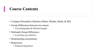
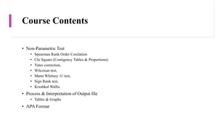
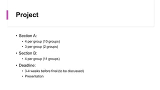
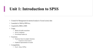
Data Analysis Using Satistical
Packages for Social Sciences
APSY 3206
Lecture 1: Dr. Rayna Sadia
Assistant Professor
Riphah International Univeristy, Islamabad
Course Objectives
• Statistical Analysis
• Basic concept of psychological research
• Grasp the concept
• Theoratical rational
• Learn the procedures to carry out certain analysis
• Enhancing competence
• For Data Processing
• Entry
• Analysis
• Interpretations
• Tables and figures
Course Outcomes
• Process Research Data
• Prepare variabvle view file
• Data entry
• Appropiate analysis
• Interpretation : output file
• Reporting
• Concise & appropiate
• Tables and graphical form
• Interpret results in reports.
Course Contents
• Introduction gto Statistical Package for Social Sciences (SPSS)
• Basic Features of SPSS
• Preparing Data for Entering in SPSS
• Preparing variable view file
• Data Entry in Data View File
• Computing & Recoding Data
Course Contents
• Compute Descriptive Statistics (Mean, Median, Mode, & SD)
• Group Differences between two means
• T-test (Independent & Matched Sample)
• Multuiple Group Differences
• F-test (One-way ANOVA)
• Relationships (correlation)
• Regression
• Prediction Hypotheses
Course Contents
• Non-Parametric Test
• Spearman Rank Order Corelation
• Chi Square (Contigency Tables & Proportions)
• Yates correction,
• Wilcoxan test,
• Mann Whitney -U test,
• Sign Rank test,
• Krushkal Wallis
• Process & Interpretation of Output file
• Tables & Graphs
• APA Format
Project
• Section A:
• 4 per group (10 groups)
• 3 per group (2 groups)
• Section B:
• 4 per group (11 groups)
• Deadline:
• 3-4 weeks before final (to be discussed)
• Presentation
Unit 1: Introduction to SPSS
• Created for Management & statistical analysis of social science data
• Launched in 1968 by SPSS inc.,
• Acquired by IBM in 2009.
• Usage:
• Market & health researchers
• Survey companies
• Government bodies etc
• Functions:
• Numerous basic & complex functions
• Frequencies to factor analysis
• Grpahical representation of results
• Comaptibility
• Excel , Amos, M Plus
Basic Terminologies
• Statistics
• Dealing with number & data
• Involves activities
• Data collection from surveys / experiment
• Summarization / management of data
• Presentation of results in a suitable & convincing format
• Analysis of collected data
• Draw valid inferences from findings
• Variable
• Characteristics which varies
• Measurement / observations
• Scale
• Device on which observations are taken
• Ratings (likert type: strongly agree to disagree; Categorical: age; dicotomous: yes/no)
Basic Terminologies
• Data
• Set of observations taken form experiemnt/ survey/ external source of a specific variable using
some appropiate measurement scale
• Type of data
• Qualitative (Categorical)
• Nominal
• Ordinal
• Quantitative (Numerical)
• Discrete
• Continuous
• Data Analysis
Type of Data
Data
Categorical
Nominal Data
Ordinal Data
Metric
Discrete
Continuous
Categorical
• Nominal
• Classes or categories: no meaningful order of classes
• No hierarchy
• Blood type / sex / rural, urban residence / alive, dead / smoking status
• Ordinal
• Meaningful order of classes or categories
• Data has hierarchy
• Pain ratings / satisfaction rating / mood / socioeconomic status
Numerical
• Continuous (real-valued)
• Infinite options
• In continuity
• Age / weight / blood pressure
• Discrete (countable)
• Finite options
• Shoe size / number of cigrattes in a pack /
Scales of Measurement
• Nominal
• Numbers identify & classify objects
• No of football players
• Percentages, mode
• Chi square, binomial tests
• Ordinal
• Numbers
• Indicate relative positions of objects but nit the magnitude of differences between them
• Ranking in a tournament
• Percentile, median,
• Rank order corelation, ANOVA
Scales of Measurement
• Interval
• Equal differences between objects
• Zero has no real meanings & meanings change when unit change
• For example: temperature in Celsius and Kelvin
• Range, Mean, SD
• Product moment corelation
• Ratio
• Zero point is fixed,
• Absolute zero cease to exist
• Zero has real meaning & meaning remains same even units change
• Length in cm & m / weight in kg and pounds
• Geometric mean
• Coefficient of variation
Nominal
• Numbers serve only as lables or tags for identifying & classifying objects
• Frequencies, proportion & percentage
• Pie & Bar Chart
• Strict one to one correspendene between numbers & objects
• Numbers do not reflect the amount of characteristic possessed by the objects
• Only permissible operation on the numbers in a nominal scale is counting
• Passport number, hockey players, brands, attributes
Ordinal
• Ranking sclae
• numbers are assigned to objects to indicate the relative extent to which the objects possess some
characteristics
• Determine the relative cahracteristics of objects but not in terms of quantity (less or
high)
• Relative position not the magnitude of differences between the objects
• Permits the operation of statistics based on
• Percentile, quartile, median
• Possess description & order not distance or origin
Interval
• Numerically equal distances on the scales represents equal values in the
characteristics being measured.
• Permits comaprison of the differences between objects
• Location of zero point is not fixed
• Everyday tempeature scale
• Attitudinal data obtained on rating scales.
Ratio
• The highest scale allows to identify objects, rank order of objects, & comapre
intervals or differences
• Possess all properties of nominal, ordinal, and interval scales
• Has an absolute zero point
• All statistical techniques can be applied to ratio data
• Height, weight, age, money, market share, number of customers
Parametic / Non Parametric Data
• Ranks , scores, or categories are generally non-parametric data
• When in doubt (especially with small sample size)
• Drawback: high chances of missing a small effect detect a small effect that
does exist
• Measurements that come from a population that is normally
distributed can usually be treated as parametric
• Normal data distribution: more values near mean and gradually less far
away symmetrically
Steps in Data Analysis
• Questionnaire check / Data Preparation
• Coding
• Cleaning data
• Appropiate tools for analysis
Questionnaire Check
• Returned questionnaire unaccepatble for many reasons
• Incomplete questionnaire
• Pattern of responses
• Responents couldn’t understand or follow the instructions
• Responses
• Little variance
• Missing pages
• Respondent doesnot qualify for participation
Data Preparation
• Conversion of raw data into usable data
• Coding
• Transformation of information from questionnaire to dataabase
• Results depend on quality of data
• Possiblities of errors
• Handling instruments
• Raw data
• Transcribing
• Data entry
• Assigning codes
• Values
• Value lables
• Data needs to be clean
Coding
• Assigning a code, usually a number, to each possible response to each
question
• Gender:
• Male = 0, Female = 1
• Marital status
• Single = 0, Married = 1, widowed = 2, divorced = 3
• Education
• Residence
• Age
Data Cleaning
• The very first step before analyzing data
• Outliers
• Really high / low values
• Age = 110 (it might be 1just 10 or 11)
• Value entered that doesnot exist for variable?
• 2 entered where 1= male, 0 = female
• Missing values
• Not responded
• Accidently provided answer
• Data not entered into the database
Basic Feature of SPSS
• Statistical package for data analysis in social & medical sciences
• Founded in 1968
• More than 250,000 users worldwide
• 1200 employee in 60 countries
• Owned by IBM
• PASW (Predictive Analytics software)
• Translate the questionnaire into codes & enter into SPSS
• Questionnaires are mapped
• As variables in SPSS
• Important factors to be considered before entering data
• Question response formats
• Scale characteristics
• Level of measurement
Questionnaire Formats
• Close ended
• Open ended with numeric repsonse
• open ended with text response
• Multiple response questions
• Convert all of them into numeric or string data for entering into SPSS
• For example
• To what extent you are staisfied with the lecture so far
• Very satisfied, satisfied, disstisfied, very dissatified
• 4, 3, 2, 1
Response formats
• Close ended:
• Gender
• Male, (0)
• Female (1)
• Open ended numerical
• Avergae expenditure of groceries on weekly basis ……..
• How many years you have been working here…..
• Open ended with text reposne
• What would you like to change about this product…
• coding manually afterwards
• Type the answers
Unit 2: Lecture 3
Launching SPSS
SPSS Windows
• No of different types of windows
• Active window
• Currently working
• Data editor window
• Display content of the data file
• Opens automatically when you open SPSS
• Create new data file / modify an existing one
• Provides two view of the data
Data Editor window
• Data view file:
• Displays dta values
• Variable is a column
• Row is a case
• Variable View
• Table consisting of variable names & their attributes
• Properties of each variable can be modified
• Add / delete existing variable in the variable view windows
Viewer Window
• Displays statistical results, Tables, charts
• Opens automaticallly the first time you run a procedure that generates ouput.
Purpose of different menus
• File Menu
• Open several existing files or a database like in excel/ save changes
• Edit Menu
• Cut, copy, paste, insert variable, insert cases
• Data Menu
• Define variable properties, sort cases, merge files, spilt files, select cases
• Transform Menu
• Computations
• Create new variable for existing / recode old variable
Conti--
• Analyze Menu
• All statistical analysis takes place
• Descriptive sttistics to non-parametric tests
• Graph Menu
• Create plots & graphs
• Can be edited in chart editor window
• Utilities Menu
• Run scripts / syntax
• Display information on the contents of SPSS dta files
Conti..
• Extensions
• Extensions that allows to integrates higher program like R & python into SPSS
• Separate purchasing
• Window
• Change active window
• Window with the check mark is the active one (data editor window)
• Help
• Help on topics in SOSS
• Ask statistics coach some basic questionss.
Toolbars
• Each window has its own toolbar
• Provides access to common tasks
• Some windows have more than one
• Pointer on the tool provides description of the tool
• You can show move or hide the toolbar
Status Bars
• At the bottom of each SPSS
• Command status
• Provides information of a running procedure
• Filter status
• Dispalys when a subset of cases are used for analysis
• Weight status
• Weight variable is being used
• Split file status
• When file has been splited into two groups
Dialogue Boxes
• Many menu selections have dialogue boxes
• Select variables & options for analysis
• Main dialogue box
• Source variable
• List of variable type from the working data file
• Target variable
• One/more lists of variables needed for the analysis
• Command push buttons
• Run the procedure by opening a dialogue box
Command push buttons
• Ok
• To run the procedure in a dialogue box
• Paste
• Click this button to generate a command syntax from your selections
• Command syntax is then pasted into syntax window
• Modified for future analysis
• This creates the code known as SPSS program
• Reset
• Deselects any sections, & reset all specifications in the dialog box
Conti…
• Cancel
• Cancels any change in the dialog box since the last time it opened
• Close thr dialoge box
• Help:
• Provides help about the current dialog box
Create a New data Set
• Defining varibales in the varibale view
• Variable anme
• Variable type
• Variable label
• Missing Values
• Allignment
• Scale
• Variable view in data view
• Rows of variable views appear as column in data view
Variable Name
• Each variable name must be unique
• Must starts with a letter
• Upto 8 characters
• Letters, numbers, &underscore ( _ )
• Certain keywords can not be used
• Compute, sum, average
• Varibale name can be changed
• Highlight the variable name by clicking it and type new one
Conti..
• Create new variable
• click first empty row under the name column and type new name
• “Cat_dog” can be used but not
• “cat-dog” / “cat dog”
• Hyphen ( -) will be interpreted by SPSS as negative sign or subtraction
• Space confuses SPSS as to how many variables are being named
Variable Type
• Two basic types of variable
• Numeric
• Only number assigned
• String
• May contain letters / number
• Even if numbers are allowed
• Numberic operations cannot be allowed
• Mean, median, variance, SD,
• Varibale type can be changes
• width of the string can be changed
Decimals
• Number of the decimal places that SPSS will display
• If more decimals are entered
• Information will be retained but not displayed
• For whole numbers reduce the decimals to zero
• Can be changed into desired decimals
Variable Label
• String of text to identify the variable in more detail of what a variable
respresents
• Name
• Limited to 255 chaaracters
• May contain space and punctuation
• Can be changed
Values
• Code of the answer
• labels to specific values
• response formats
• assigning numbers to response formats
• (both alphabet and numbers can appear in data window)
• assign numbers to the answer
• added via dialogue box (Add / Change / Remove)
• write values and labels and click add and ok
Missing
• Signaling SPSS to treat some missing data
• other numerical value instead of data
• by default single dot by SPSS
• System Missing data
• declared value in the dialogue box
• for example 9 / 99 / 001
• SPSS will ignore these values while doing analysis
Columns
• Width of the column for each variable
• in data view
• width is different than column
• width indicate the number of digits displayed
• column size indicates the space allocated to the variable
Allign
• the adjustemnt of data with in column
• left / right / Centre / justified
Measure
• Level of Measurement
• SPSS doesnot diffeerentiate between interval & ratio scale
• boh categorized as SCALE in SPSS
• However, nominal and ordinal are differnetiated
Entering Data into SPSS
• Enter, save, edit data in SPSS
• define all variables
• name the variable
• specifically scale of measurement
• type of data
• assigning labels to variables & data values
• finish Variable view
• start entering data into SPSS
• Save data file
• .sav file
Unit 3
Activity
• Data Entry into SPSS
• Class practice
• Questionnaire & code book
Unit 4 & 5: File Management
• Summarize SPSS
• Missing
• Transform
• Select
• Split
• Compute new variables
• merging files
• Sorting transpose
• weighted cases
Storing & Retrieving Files
• Always save the changes in the data file
• Data Files
• Menu
• Save file (.sav)
• always save the changes in the current file
• Save as
• save changes in the new fiel / locations
• other extensions
• ASCII text (.dat)
• Excel (.xls)
• dBASE (.dbf)
Open & Retrieve
• Open an existing file
• open new file
• open recently used file
• Import file
• all the supporting files
• excel
• database
• ASCII
importing an excel file
• File
• import data
• excel
• preview of the file
• if multiple sheets select number of sheet
from sheet lists
Missing Values
• Missing or invalid data
• Refuse to respond
• Do not know the answer
• Answer in an unexpected format
• Empty data fields / fields containing invalid entries are converted into system-missing, which is
identifiable by a single period
• Add number & label to the missing value,
• 999
• label (No response)
• for string
• NR
• Label (No Response)
• Case Sensitive (nr wont be treated as a missing values)
Handling Missing Values
• Some analysis can’t be carried out with missing values
• Ways to handle missing values
• Arithmetic mean
• Mean of nearby points
• Median of near by points
• Linear interpolation
• Linear trend at point
• Assignment: which one is the best method to handle missing & why
Sort Cases
• open file
• data
• sort cases
• select varaibe
• sort according to varaibale
Check Outliers
• identify unusual cases in the data file
• min or max value than response format
• by taking frequencies
• sorting data ascending / descending
• Why it is important to assess outliers in the data
Modifying Data Value
• create a categorical variable from a scale variable
• combine several response categories into a single category
Compute variable
• Recoding of variables
• For reverse items
• into same variables
• into different variables ( to save the original file)
• Compute
• Functions in Expressions
• More than 70 built in function (arithmetic / statistical / distribution)
Graphs
• For Qualitative data
• Frequencies & charts
• Analyze > Descriptive > Frequencies
• Chart Builder > select graph > arrange variables on x and y axis
• For Quantitative data
• Mean / SD
• Table Looks
• double click table > format > Table looks
• file > options >viewer / output > pivot tables>
SPSS Graphs
• Building charts
• Editing charts
• Formating charts in word
• Bar / histogram / linear / pie
• Pie & Bar Chart difference
• One category
• More than one category
Exporting Results to other formats
• copy paste
• As formatted / unformatted text
• file > export > word / excel / pdf
working with syntax
• Importance of syntax
• Existing syntax
• file> open > synatx
• *.sps
• run menu to run the syntax
• select command
• paste rather ok
• Using breaking points
• click any where to the left of text
• represented as a red circle
• execution stops at the red points
• Double click > clear breaking point
• Run> continue

APSY3206 Lecture 1.pptx

  • 1.
    Data Analysis UsingSatistical Packages for Social Sciences APSY 3206 Lecture 1: Dr. Rayna Sadia Assistant Professor Riphah International Univeristy, Islamabad
  • 2.
    Course Objectives • StatisticalAnalysis • Basic concept of psychological research • Grasp the concept • Theoratical rational • Learn the procedures to carry out certain analysis • Enhancing competence • For Data Processing • Entry • Analysis • Interpretations • Tables and figures
  • 3.
    Course Outcomes • ProcessResearch Data • Prepare variabvle view file • Data entry • Appropiate analysis • Interpretation : output file • Reporting • Concise & appropiate • Tables and graphical form • Interpret results in reports.
  • 4.
    Course Contents • Introductiongto Statistical Package for Social Sciences (SPSS) • Basic Features of SPSS • Preparing Data for Entering in SPSS • Preparing variable view file • Data Entry in Data View File • Computing & Recoding Data
  • 5.
    Course Contents • ComputeDescriptive Statistics (Mean, Median, Mode, & SD) • Group Differences between two means • T-test (Independent & Matched Sample) • Multuiple Group Differences • F-test (One-way ANOVA) • Relationships (correlation) • Regression • Prediction Hypotheses
  • 6.
    Course Contents • Non-ParametricTest • Spearman Rank Order Corelation • Chi Square (Contigency Tables & Proportions) • Yates correction, • Wilcoxan test, • Mann Whitney -U test, • Sign Rank test, • Krushkal Wallis • Process & Interpretation of Output file • Tables & Graphs • APA Format
  • 7.
    Project • Section A: •4 per group (10 groups) • 3 per group (2 groups) • Section B: • 4 per group (11 groups) • Deadline: • 3-4 weeks before final (to be discussed) • Presentation
  • 8.
    Unit 1: Introductionto SPSS • Created for Management & statistical analysis of social science data • Launched in 1968 by SPSS inc., • Acquired by IBM in 2009. • Usage: • Market & health researchers • Survey companies • Government bodies etc • Functions: • Numerous basic & complex functions • Frequencies to factor analysis • Grpahical representation of results • Comaptibility • Excel , Amos, M Plus
  • 9.
    Basic Terminologies • Statistics •Dealing with number & data • Involves activities • Data collection from surveys / experiment • Summarization / management of data • Presentation of results in a suitable & convincing format • Analysis of collected data • Draw valid inferences from findings • Variable • Characteristics which varies • Measurement / observations • Scale • Device on which observations are taken • Ratings (likert type: strongly agree to disagree; Categorical: age; dicotomous: yes/no)
  • 10.
    Basic Terminologies • Data •Set of observations taken form experiemnt/ survey/ external source of a specific variable using some appropiate measurement scale • Type of data • Qualitative (Categorical) • Nominal • Ordinal • Quantitative (Numerical) • Discrete • Continuous • Data Analysis
  • 11.
    Type of Data Data Categorical NominalData Ordinal Data Metric Discrete Continuous
  • 12.
    Categorical • Nominal • Classesor categories: no meaningful order of classes • No hierarchy • Blood type / sex / rural, urban residence / alive, dead / smoking status • Ordinal • Meaningful order of classes or categories • Data has hierarchy • Pain ratings / satisfaction rating / mood / socioeconomic status
  • 13.
    Numerical • Continuous (real-valued) •Infinite options • In continuity • Age / weight / blood pressure • Discrete (countable) • Finite options • Shoe size / number of cigrattes in a pack /
  • 14.
    Scales of Measurement •Nominal • Numbers identify & classify objects • No of football players • Percentages, mode • Chi square, binomial tests • Ordinal • Numbers • Indicate relative positions of objects but nit the magnitude of differences between them • Ranking in a tournament • Percentile, median, • Rank order corelation, ANOVA
  • 15.
    Scales of Measurement •Interval • Equal differences between objects • Zero has no real meanings & meanings change when unit change • For example: temperature in Celsius and Kelvin • Range, Mean, SD • Product moment corelation • Ratio • Zero point is fixed, • Absolute zero cease to exist • Zero has real meaning & meaning remains same even units change • Length in cm & m / weight in kg and pounds • Geometric mean • Coefficient of variation
  • 16.
    Nominal • Numbers serveonly as lables or tags for identifying & classifying objects • Frequencies, proportion & percentage • Pie & Bar Chart • Strict one to one correspendene between numbers & objects • Numbers do not reflect the amount of characteristic possessed by the objects • Only permissible operation on the numbers in a nominal scale is counting • Passport number, hockey players, brands, attributes
  • 17.
    Ordinal • Ranking sclae •numbers are assigned to objects to indicate the relative extent to which the objects possess some characteristics • Determine the relative cahracteristics of objects but not in terms of quantity (less or high) • Relative position not the magnitude of differences between the objects • Permits the operation of statistics based on • Percentile, quartile, median • Possess description & order not distance or origin
  • 18.
    Interval • Numerically equaldistances on the scales represents equal values in the characteristics being measured. • Permits comaprison of the differences between objects • Location of zero point is not fixed • Everyday tempeature scale • Attitudinal data obtained on rating scales.
  • 19.
    Ratio • The highestscale allows to identify objects, rank order of objects, & comapre intervals or differences • Possess all properties of nominal, ordinal, and interval scales • Has an absolute zero point • All statistical techniques can be applied to ratio data • Height, weight, age, money, market share, number of customers
  • 20.
    Parametic / NonParametric Data • Ranks , scores, or categories are generally non-parametric data • When in doubt (especially with small sample size) • Drawback: high chances of missing a small effect detect a small effect that does exist • Measurements that come from a population that is normally distributed can usually be treated as parametric • Normal data distribution: more values near mean and gradually less far away symmetrically
  • 21.
    Steps in DataAnalysis • Questionnaire check / Data Preparation • Coding • Cleaning data • Appropiate tools for analysis
  • 22.
    Questionnaire Check • Returnedquestionnaire unaccepatble for many reasons • Incomplete questionnaire • Pattern of responses • Responents couldn’t understand or follow the instructions • Responses • Little variance • Missing pages • Respondent doesnot qualify for participation
  • 23.
    Data Preparation • Conversionof raw data into usable data • Coding • Transformation of information from questionnaire to dataabase • Results depend on quality of data • Possiblities of errors • Handling instruments • Raw data • Transcribing • Data entry • Assigning codes • Values • Value lables • Data needs to be clean
  • 24.
    Coding • Assigning acode, usually a number, to each possible response to each question • Gender: • Male = 0, Female = 1 • Marital status • Single = 0, Married = 1, widowed = 2, divorced = 3 • Education • Residence • Age
  • 25.
    Data Cleaning • Thevery first step before analyzing data • Outliers • Really high / low values • Age = 110 (it might be 1just 10 or 11) • Value entered that doesnot exist for variable? • 2 entered where 1= male, 0 = female • Missing values • Not responded • Accidently provided answer • Data not entered into the database
  • 26.
    Basic Feature ofSPSS • Statistical package for data analysis in social & medical sciences • Founded in 1968 • More than 250,000 users worldwide • 1200 employee in 60 countries • Owned by IBM • PASW (Predictive Analytics software)
  • 27.
    • Translate thequestionnaire into codes & enter into SPSS • Questionnaires are mapped • As variables in SPSS • Important factors to be considered before entering data • Question response formats • Scale characteristics • Level of measurement
  • 28.
    Questionnaire Formats • Closeended • Open ended with numeric repsonse • open ended with text response • Multiple response questions • Convert all of them into numeric or string data for entering into SPSS • For example • To what extent you are staisfied with the lecture so far • Very satisfied, satisfied, disstisfied, very dissatified • 4, 3, 2, 1
  • 29.
    Response formats • Closeended: • Gender • Male, (0) • Female (1) • Open ended numerical • Avergae expenditure of groceries on weekly basis …….. • How many years you have been working here….. • Open ended with text reposne • What would you like to change about this product… • coding manually afterwards • Type the answers
  • 30.
  • 31.
  • 32.
    SPSS Windows • Noof different types of windows • Active window • Currently working • Data editor window • Display content of the data file • Opens automatically when you open SPSS • Create new data file / modify an existing one • Provides two view of the data
  • 33.
    Data Editor window •Data view file: • Displays dta values • Variable is a column • Row is a case • Variable View • Table consisting of variable names & their attributes • Properties of each variable can be modified • Add / delete existing variable in the variable view windows
  • 34.
    Viewer Window • Displaysstatistical results, Tables, charts • Opens automaticallly the first time you run a procedure that generates ouput.
  • 36.
    Purpose of differentmenus • File Menu • Open several existing files or a database like in excel/ save changes • Edit Menu • Cut, copy, paste, insert variable, insert cases • Data Menu • Define variable properties, sort cases, merge files, spilt files, select cases • Transform Menu • Computations • Create new variable for existing / recode old variable
  • 37.
    Conti-- • Analyze Menu •All statistical analysis takes place • Descriptive sttistics to non-parametric tests • Graph Menu • Create plots & graphs • Can be edited in chart editor window • Utilities Menu • Run scripts / syntax • Display information on the contents of SPSS dta files
  • 38.
    Conti.. • Extensions • Extensionsthat allows to integrates higher program like R & python into SPSS • Separate purchasing • Window • Change active window • Window with the check mark is the active one (data editor window) • Help • Help on topics in SOSS • Ask statistics coach some basic questionss.
  • 39.
    Toolbars • Each windowhas its own toolbar • Provides access to common tasks • Some windows have more than one • Pointer on the tool provides description of the tool • You can show move or hide the toolbar
  • 40.
    Status Bars • Atthe bottom of each SPSS • Command status • Provides information of a running procedure • Filter status • Dispalys when a subset of cases are used for analysis • Weight status • Weight variable is being used • Split file status • When file has been splited into two groups
  • 41.
    Dialogue Boxes • Manymenu selections have dialogue boxes • Select variables & options for analysis • Main dialogue box • Source variable • List of variable type from the working data file • Target variable • One/more lists of variables needed for the analysis • Command push buttons • Run the procedure by opening a dialogue box
  • 42.
    Command push buttons •Ok • To run the procedure in a dialogue box • Paste • Click this button to generate a command syntax from your selections • Command syntax is then pasted into syntax window • Modified for future analysis • This creates the code known as SPSS program • Reset • Deselects any sections, & reset all specifications in the dialog box
  • 43.
    Conti… • Cancel • Cancelsany change in the dialog box since the last time it opened • Close thr dialoge box • Help: • Provides help about the current dialog box
  • 44.
    Create a Newdata Set • Defining varibales in the varibale view • Variable anme • Variable type • Variable label • Missing Values • Allignment • Scale • Variable view in data view • Rows of variable views appear as column in data view
  • 46.
    Variable Name • Eachvariable name must be unique • Must starts with a letter • Upto 8 characters • Letters, numbers, &underscore ( _ ) • Certain keywords can not be used • Compute, sum, average • Varibale name can be changed • Highlight the variable name by clicking it and type new one
  • 47.
    Conti.. • Create newvariable • click first empty row under the name column and type new name • “Cat_dog” can be used but not • “cat-dog” / “cat dog” • Hyphen ( -) will be interpreted by SPSS as negative sign or subtraction • Space confuses SPSS as to how many variables are being named
  • 48.
    Variable Type • Twobasic types of variable • Numeric • Only number assigned • String • May contain letters / number • Even if numbers are allowed • Numberic operations cannot be allowed • Mean, median, variance, SD, • Varibale type can be changes • width of the string can be changed
  • 49.
    Decimals • Number ofthe decimal places that SPSS will display • If more decimals are entered • Information will be retained but not displayed • For whole numbers reduce the decimals to zero • Can be changed into desired decimals
  • 50.
    Variable Label • Stringof text to identify the variable in more detail of what a variable respresents • Name • Limited to 255 chaaracters • May contain space and punctuation • Can be changed
  • 51.
    Values • Code ofthe answer • labels to specific values • response formats • assigning numbers to response formats • (both alphabet and numbers can appear in data window) • assign numbers to the answer • added via dialogue box (Add / Change / Remove) • write values and labels and click add and ok
  • 52.
    Missing • Signaling SPSSto treat some missing data • other numerical value instead of data • by default single dot by SPSS • System Missing data • declared value in the dialogue box • for example 9 / 99 / 001 • SPSS will ignore these values while doing analysis
  • 53.
    Columns • Width ofthe column for each variable • in data view • width is different than column • width indicate the number of digits displayed • column size indicates the space allocated to the variable
  • 54.
    Allign • the adjustemntof data with in column • left / right / Centre / justified
  • 55.
    Measure • Level ofMeasurement • SPSS doesnot diffeerentiate between interval & ratio scale • boh categorized as SCALE in SPSS • However, nominal and ordinal are differnetiated
  • 56.
    Entering Data intoSPSS • Enter, save, edit data in SPSS • define all variables • name the variable • specifically scale of measurement • type of data • assigning labels to variables & data values • finish Variable view • start entering data into SPSS • Save data file • .sav file
  • 57.
  • 58.
    Activity • Data Entryinto SPSS • Class practice • Questionnaire & code book
  • 59.
    Unit 4 &5: File Management • Summarize SPSS • Missing • Transform • Select • Split • Compute new variables • merging files • Sorting transpose • weighted cases
  • 60.
    Storing & RetrievingFiles • Always save the changes in the data file • Data Files • Menu • Save file (.sav) • always save the changes in the current file • Save as • save changes in the new fiel / locations • other extensions • ASCII text (.dat) • Excel (.xls) • dBASE (.dbf)
  • 61.
    Open & Retrieve •Open an existing file • open new file • open recently used file • Import file • all the supporting files • excel • database • ASCII
  • 62.
    importing an excelfile • File • import data • excel • preview of the file • if multiple sheets select number of sheet from sheet lists
  • 63.
    Missing Values • Missingor invalid data • Refuse to respond • Do not know the answer • Answer in an unexpected format • Empty data fields / fields containing invalid entries are converted into system-missing, which is identifiable by a single period • Add number & label to the missing value, • 999 • label (No response) • for string • NR • Label (No Response) • Case Sensitive (nr wont be treated as a missing values)
  • 64.
    Handling Missing Values •Some analysis can’t be carried out with missing values • Ways to handle missing values • Arithmetic mean • Mean of nearby points • Median of near by points • Linear interpolation • Linear trend at point • Assignment: which one is the best method to handle missing & why
  • 65.
    Sort Cases • openfile • data • sort cases • select varaibe • sort according to varaibale
  • 66.
    Check Outliers • identifyunusual cases in the data file • min or max value than response format • by taking frequencies • sorting data ascending / descending • Why it is important to assess outliers in the data
  • 67.
    Modifying Data Value •create a categorical variable from a scale variable • combine several response categories into a single category
  • 68.
    Compute variable • Recodingof variables • For reverse items • into same variables • into different variables ( to save the original file) • Compute • Functions in Expressions • More than 70 built in function (arithmetic / statistical / distribution)
  • 69.
    Graphs • For Qualitativedata • Frequencies & charts • Analyze > Descriptive > Frequencies • Chart Builder > select graph > arrange variables on x and y axis • For Quantitative data • Mean / SD • Table Looks • double click table > format > Table looks • file > options >viewer / output > pivot tables>
  • 70.
    SPSS Graphs • Buildingcharts • Editing charts • Formating charts in word • Bar / histogram / linear / pie • Pie & Bar Chart difference • One category • More than one category
  • 71.
    Exporting Results toother formats • copy paste • As formatted / unformatted text • file > export > word / excel / pdf
  • 72.
    working with syntax •Importance of syntax • Existing syntax • file> open > synatx • *.sps • run menu to run the syntax • select command • paste rather ok • Using breaking points • click any where to the left of text • represented as a red circle • execution stops at the red points • Double click > clear breaking point • Run> continue

Editor's Notes

  • #20 Typically only data from last two might be suitable for parametric tests But its not a straightforward decision It is reasonable to justify the choice of analysis Analysis should be appropriate to data rather than that best suited hypotheses
  • #21 1. Before choosing a statistical test to apply to your data address whether data is parametric or not. 2.. To sensibly apply parametric tests, data should be normally distributed 3. Tests that depend on an assumption about the distribution of the underlying population data, (e.g. t-tests) are parametric because they assume that the data being tested come from a normally distributed population (i.e. a population we know the parameters of). Tests for the significance of correlation involving Pearson's product moment correlation coefficient involve similar assumptions. 4. Tests that do not depend on many assumptions about the underlying distribution of the data are called non-parametric tests the Wilcoxon signed rank test, and the Mann-Whitney test and Spearman's rank correlation coefficient. They are used widely to test small samples of ordinal data.