Definition of Linear Regression

2. Definition of Linear Regression
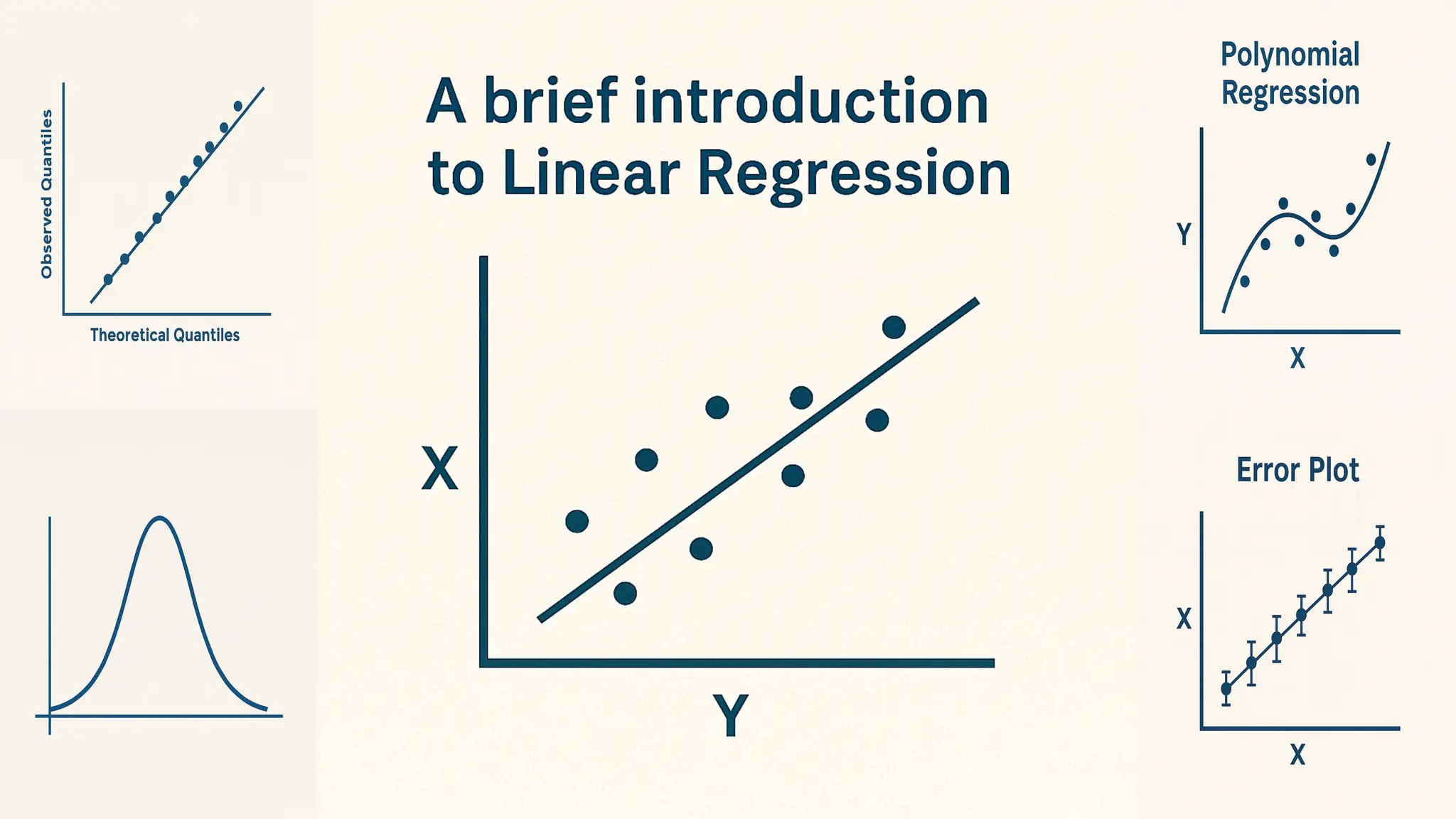
• Linear regression is a statistical method used to model the
relationship between a dependent variable and one or more
independent variables by fitting a linear equation to observed data.
• In simple linear regression, the relationship between the dependent
variable y and a single independent variable x is modeled using a
linear equation of the form:
Here, = y intercept of the line.
= Slope, which measures the avg increase/decrease in y for 1
unit
change in x.
= Error term

3. Multiple Linear Regression
• Multiple linear regression involves more than one independent
variable, and the model is expressed as:
are the coefficients of … respectfully.

4. Least Square Method
• The least squares method is the standard approach used in simple
linear regression to estimate the parameters (coefficients) of the
model.
• Model Equation:
• Sample Estimate Equation:
• Objective function:

5. Least Square Method
• Partial Derivatives:
and
To find the values of the coefficients, we need to minimize the
error term i.e. the equations will be equal to zero. When the error
term will be minimized, then the slope of the parabola will be equal
to zero, which parabola was created taking the value of coefficient on
the x axis and the value of error on y axis.

6. Coefficients
• By mathematical derivation we get,
By these two equations, we calculate the values of the coeffi-
cients from a sample.

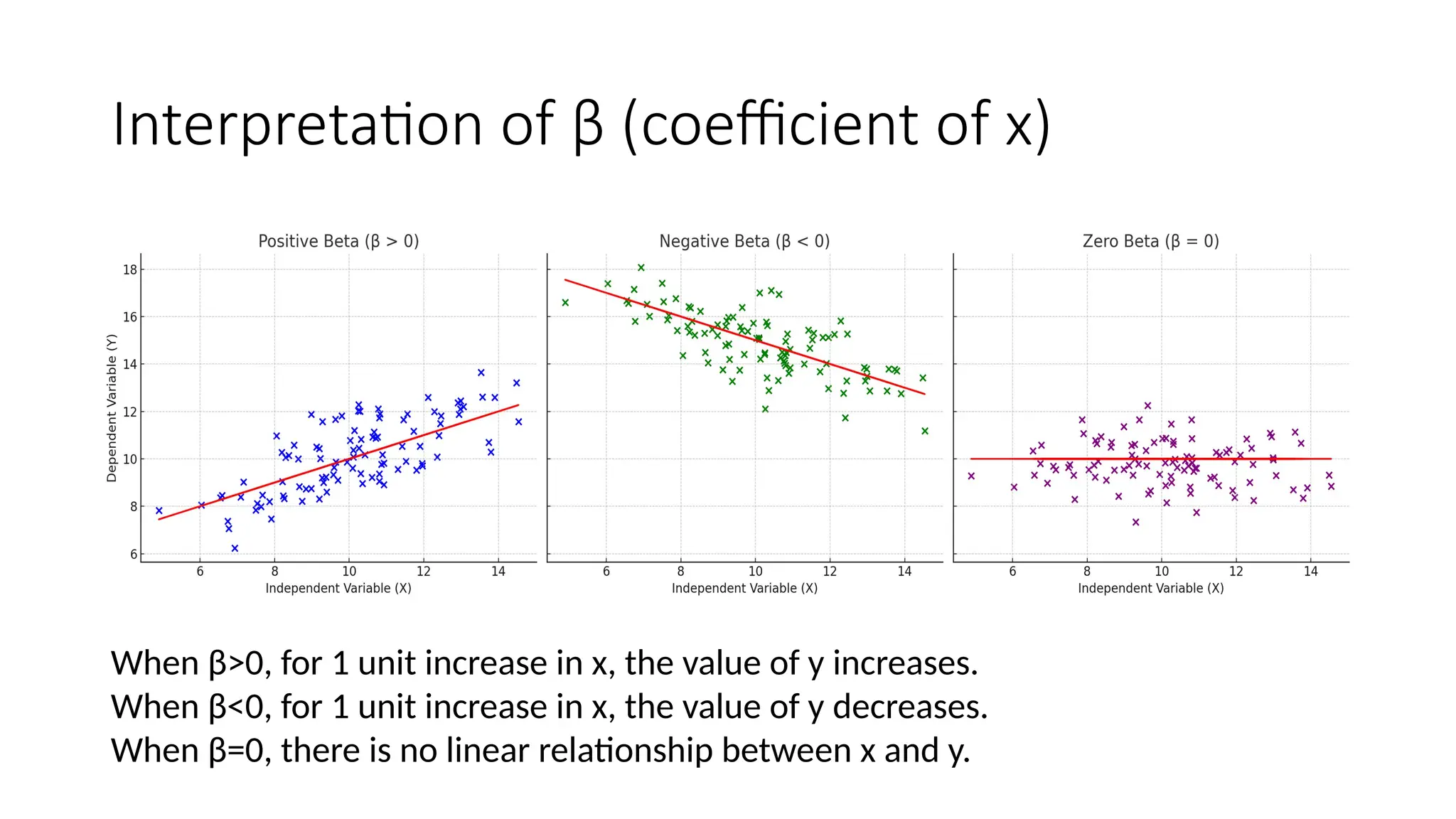
7. Interpretation of β (coefficient of x)
When β>0, for 1 unit increase in x, the value of y increases.
When β<0, for 1 unit increase in x, the value of y decreases.
When β=0, there is no linear relationship between x and y.

8. Example
• The dataframe where y is the dependent variable and xs are
independent variables:

9. Multiple Linear Regression Summary

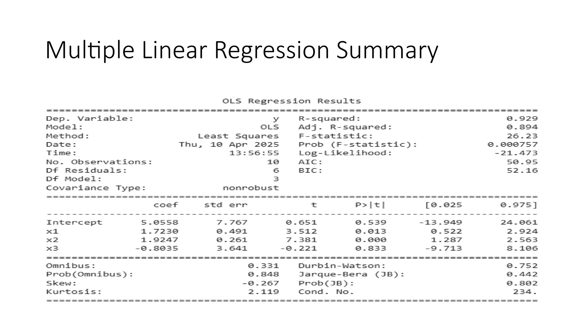
10. Interpretation
• Here, the value is 0.929. This tells us, 92.9% of the variance in the
dependent variable y is explainable by the independent variables.
• The p value (Probability of accepting a null hypothesis) of the t test for
is 0.013 < 0.05, for is 0.000 < 0.05 and for is 0.833 > 0.05.
• So, the two independent variables and has significant effect to
explain the variability in y, thus, they have significant effect to predict
y by the regression model. (in 5% level of significance)
• And does not have significant effect to explain the variability in y.

11. Interpretation
• The adjusted value is, 0.894. Thus, 89.4% variability of the depen-
dent variable y can be explained by and because they have
significant effects to predict y.
• Only 0.929-0.894 = 0.035, thus 3.5% of the variability in y can be
explained by which we can ignore and we can drop the variable
to reduce the dimensionality. Often dimensionality reduction is
needed for real data because the number of independent variable
may be large.

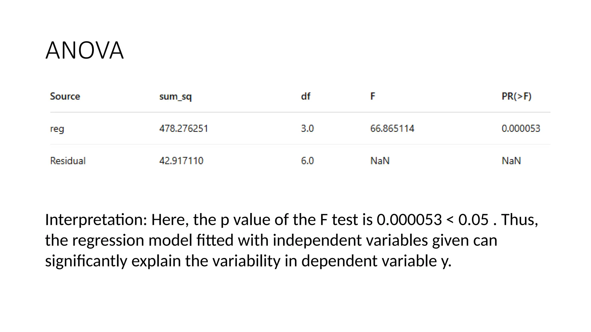
12. ANOVA
Interpretation: Here, the p value of the F test is 0.000053 < 0.05 . Thus,
the regression model fitted with independent variables given can
significantly explain the variability in dependent variable y.