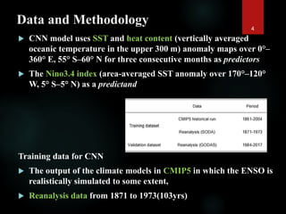
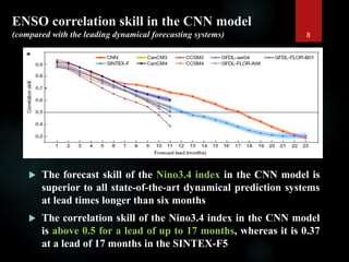
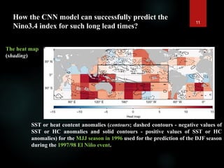
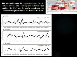
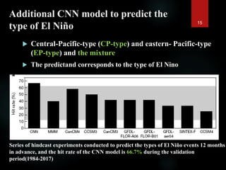
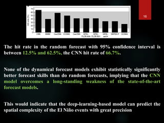
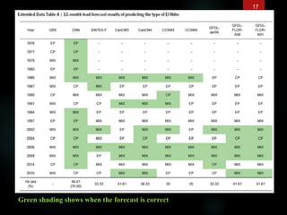
This document summarizes a study that used a deep learning convolutional neural network (CNN) to produce multi-year forecasts of El Niño Southern Oscillation (ENSO) events. The CNN model was trained on sea surface temperature and heat content anomaly data from climate models and reanalysis data from 1871 to 1973. It achieved correlation skills for ENSO forecasts up to 17 months ahead, outperforming other dynamical forecasting systems. The CNN also predicted the types of El Niño events with a 66.7% hit rate 12 months ahead, identifying precursors not previously reported. However, the limited observational record poses a challenge for applying deep learning to climate forecasts.

1. Deep learning for multi-year
ENSO forecasts
Authors: Yoo-Geun Ham, Jeong-Hwan Kim & Jing-Jia Luo
Journal: Letters, Nature(2019)
Presented by
RAKESH S
JRF, IITM

2. Introduction
 ENSO are associated with a wide range of climate
extremes and ecosystem impacts.
 Long-lead forecast for ENSO is necessary for managing
policy responses.
 ENSO forecast of lead time more than 1yr still remains
problematic.
 This study shows that a statistical forecast model using
deep-learning approach – Convolutional Neural
Network(CNN) can produce skill upto one and half yrs.
2

3. CNN architecture
 Predictor(input) – SST,HC anomaly
 Convolutional filter - extracts the
rich regional features
 3 Convolutional layers
* All figures in the slides are taken from the ref. journal
3
The 3 month-averaged Nino3.4 index from time τ + 1 month
to τ + 23 months is used as a variable for the output layer.
 2 Max-pooling layers - enhance the
value of feature
 Fully connected layer
 Predictand(output)

4. Data and Methodology
 CNN model uses SST and heat content (vertically averaged
oceanic temperature in the upper 300 m) anomaly maps over 0°–
360° E, 55° S–60° N for three consecutive months as predictors
 The Nino3.4 index (area-averaged SST anomaly over 170°–120°
W, 5° S–5° N) as a predictand
Training data for CNN
 The output of the climate models in CMIP5 in which the ENSO is
realistically simulated to some extent,
 Reanalysis data from 1871 to 1973(103yrs)
4

5. Methodology - Convolutional process
 The convolutional process of the CNN involves the extraction
of local characteristics from the global maps, and the
calculation of dot products between values in the
convolutional filter and those in the input layer. The output of
the convolutional process is then translated into a feature
map.
 The values of the convolutional filter are determined
automatically by iteration by minimizing the cost function,
defined as the mean squared difference between the predicted
and true distributions
5

6. Methodology - Transfer learning technique
- Circumvent the limited amount of observational data
 This technique uses the knowledge acquired from a similar
task with a larger number of samples for performing the
target task.
 The model is first trained using the CMIP5 output, and then
the trained weights are used as initial weights to formulate the
final CNN model with the reanalysis
6

7. Results and Discussion
7

8. ENSO correlation skill in the CNN model
(compared with the leading dynamical forecasting systems)
 The forecast skill of the Nino3.4 index in the CNN model is
superior to all state-of-the-art dynamical prediction systems
at lead times longer than six months
 The correlation skill of the Nino3.4 index in the CNN model
is above 0.5 for a lead of up to 17 months, whereas it is 0.37
at a lead of 17 months in the SINTEX-F5
8

9. (b) Correlation skill of the Nino3.4 index targeted to each calendar month in the CNN
model and (c) SINTEX-F. Hatching highlights the forecasts with correlation skill
exceeding 0.5.
 CNN model shows a higher correlation skill of the Nino3.4 index for
almost all targeted seasons, compared to SINTEX-F
 The forecasts targeting the May–June–July (MJJ) season have
correlation skill exceeding 0.5 only up to a lead of four months in the
SINTEX-F, compared to a lead of up to 11 months in the CNN
9

10. The Nino3.4 index for DJF season for the 18-month-lead forecast
demonstrates that the CNN model correctly predicts the ENSO amplitude
10

11. SST or heat content anomalies (contours; dashed contours - negative values of
SST or HC anomalies and solid contours - positive values of SST or HC
anomalies) for the MJJ season in 1996 used for the prediction of the DJF season
during the 1997/98 El Niño event.
How the CNN model can successfully predict the
Nino3.4 index for such long lead times?
The heat map
(shading)
11

12. The anomalies over the tropical western Pacific,
Indian Ocean and subtropical Atlantic (red
shadings in HM) are the main contributors to
the successful prediction of the 1997/98 El Niño.

13. In addition to the ENSO amplitude, the global impacts
of El Niño events vary greatly according to the detailed
zonal distributions of El Niño SST anomalies
14

14. Additional CNN model to predict the
type of El Niño
 Central-Pacific-type (CP-type) and eastern- Pacific-type
(EP-type) and the mixture
 The predictand corresponds to the type of El Nino
Series of hindcast experiments conducted to predict the types of El Niño events 12 months
in advance, and the hit rate of the CNN model is 66.7% during the validation
period(1984-2017)
15

15. The hit rate in the random forecast with 95% confidence interval is
between 12.5% and 62.5%, the CNN hit rate of 66.7%.
None of the dynamical forecast models exhibit statistically significantly
better forecast skills than do random forecasts, implying that the CNN
model overcomes a long-standing weakness of the state-of-the-art
forecast models.
This would indicate that the deep-learning-based model can predict the
spatial complexity of the El Niño events with great precision
16

16. Green shading shows when the forecast is correct
17

17. Comes from: Successful extraction of features in
input variables through convolutional process
CP-type El Niño precursors in the South Pacific and the
Indian Ocean have not been reported before, and the
additional analysis shows that the identified precursors can
lead the CP-type El Niño event
This indicates that the CNN can be a powerful
tool to reveal complex ENSO mechanisms
19
Superiority

18. Limitation
 One of the biggest limitations in applying deep learning to climate
forecasts is that the observation period is too short to achieve
proper training.
 Observations of global oceanic temperature distributions are
available from 1871. This means that, for each calendar month,
the number of samples is less than 150
20

19. Thank You
Contact: srakesh@tropmet.res.in