Download to read offline

![M. A. Azarmehr / Management Science Letters 2 (2012)
47
߲ߨ
߲ݍଶ
ൌ ߙߚሾ െ ݓଵ െ ܨሺݍଵ ݍଶሻ െ ݇ܨሺݍଵ ݍଶሻ ݇ሿ ߙሺ1 െ ߚሻሾ െ ݓଶ െ ܨሺݍଶሻ െ ݇ܨሺݍଶሻ ݇ሿ
ሺ1 െ ߙሻሾ0ሿ ൌ 0 ՜ ݍଶכ
ൌ ܨିଵ ൬
ߙሺଵ െ ݓଶ ݇ሻ െ ߙߚሺଵ െ ݓଵ ݇ሻ
ߙሺ1 െ ߚሻሺଵ ݇ሻ
൰ ݀ ൌ ܨିଵሺΔሻ݀
(3)
߲ଶߨ
߲ݍଶ
ଶ ൏ 0
Thus, ߨ is strictly concave in ݍଶכ
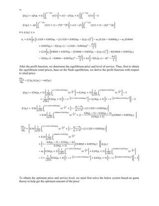
and ሺݍଵ ݍଶሻכ. Then, replacing the optimal order quantities into
Eq. (1) yields the following,
ߨሺ, ݏሻ ൌ ߙߚ ቈሺଵ ݇ሻ ቈܨିଵሺߘሻ݀ െ න ܨ ൬
ݐ
݀
൰
ிషభሺఇሻௗ
െ ݇݀ െ ݓଵሺܨିଵሺߘሻെܨିଵሺΔሻሻ݀ െ ݓଶܨିଵሺΔሻ݀ െ
ଶ
2
ߴݏଵ
ߙሺ1 െ ߚሻ ቈሺଵ ݇ሻ ቈܨିଵሺΔሻ݀ െ න ܨ ൬
ݐ
݀
൰
ிషభሺΔሻௗ
െ ݇݀ െ ݓଶܨିଵሺΔሻ݀ െ
ଶ
2
ߴݏଵ
ሺ1 െ ߙሻ
ൌ ቈߙߚሺଵ ݇ሻ න ݐ݂ ൬
ݐ
݀
൰
ிషభሺఇሻ
ߙሺ1 െ ߚሻሺଵ ݇ሻ න ݐ݂ ൬
ݐ
݀
൰
ிషభሺΔሻ
െ ݇ ݀ െ
ଶ
2
ߴݏଵ
ൌ ܳሺሻ݀ሺ, ݏሻ െ
ଶ
2
ߴݏ
(4)
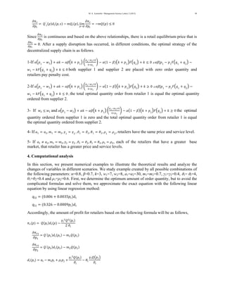
In this paper, we assume that all retailers simultaneously determine their private retail prices and
service levels. We first get the equilibrium service level based on equilibrium price, and then
determine equilibrium price. The equilibrium service level based on the Nash equilibrium is equal
with the following formula,
߲ߨ
ൌ ߛܳሺሻ െ ՜ ߲ݏ
ߴݏଵ ݏ
כ ൌ
ߛܳሺሻ
ߴ (5)
߲ଶߨ
߲ݏ
ଶ ൌ െߴ
It implies that profit function is strictly concave for any given retail price vector p and all other
retailers’ service level. Therefore, we have a unique equilibrium service level. After obtaining the
equilibrium of service level the retailer i expected demand function can be reduced as:
݀ሺሻ ൌ ܽ െ ݉ ߩ
ߛ
ଶܳሺሻ
ߴ
െ ߠ
ߛܳ൫൯
ߴ
(6)
and, we can replace the profit function as:
ߨሺሻ ൌ ܳሺሻ݀ሺሻ െ
ߛଶܳଶሺሻ
2 ߴ (7)
To obtain the equilibrium price and service level, we must first solve the below system based on the
Nash equilibrium.
߲ߨଵ
߲ଵ
ൌ 0
߲ߨଶ
߲ଶ
ൌ 0
ప
Then based on Eq. (6), the equilibrium level of service is obtained.
However, because of the difficulty of solving the exact value of the derivative to obtain the
equilibrium wholesale price and then to examine the price equilibrium behavior between retailers, we
need the following assumptions.
Assumption 1: For all i =1, 2, ..., N, the retail price is defined on ሾݓ െ ݇,ഥ], where ഥప is the
maximum price such ݀ሺሻ|ୀതതതഢ ൌ 0](https://image.slidesharecdn.com/decentralizedsupplychainsystem-141013042148-conversion-gate01/85/Decentralized-supply-chain-system-5-320.jpg)
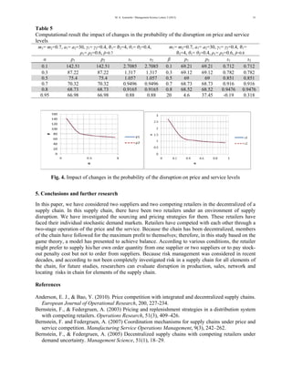

This document summarizes a research paper that presents a mathematical model of a decentralized supply chain with two suppliers and two competing retailers. The paper investigates the sourcing and pricing strategies of the two retailers under conditions of uncertain supply and supply disruptions. It reviews related literature on competition within and between supply chains. The paper then introduces a new model where the retailers face stochastic demand that depends on prices and service levels. The model accounts for the probability of supply disruptions at each supplier. Optimal order quantities and equilibrium pricing and service strategies for the retailers are then derived.


