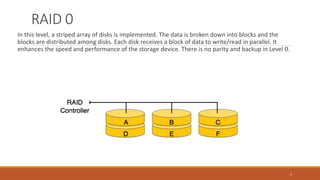
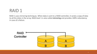
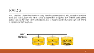
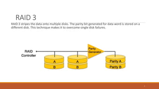
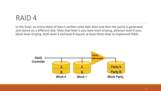
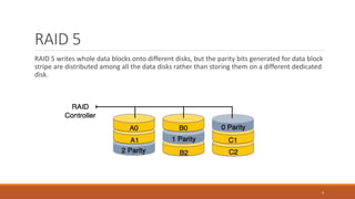
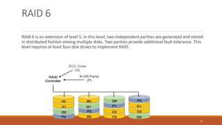
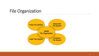
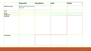
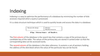
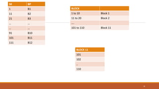
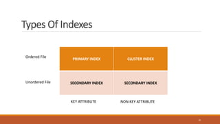
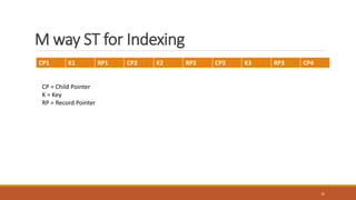
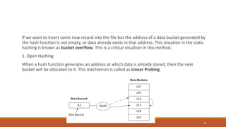
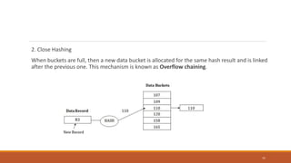
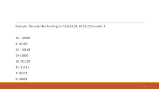
2. SYLLABUS
– RAID
– File Organization
– Organization of Records in Files
– Indexing and Hashing
–Ordered Indices
– B+ tree Index Files
– B tree Index Files
– Static Hashing
– Dynamic Hashing
– Query Processing Overview
– Algorithms for SELECT and JOIN operations
– Query optimization using Heuristics and Cost Estimation.
2
3. RAID
RAID or Redundant Array of Independent Disks, is a technology to connect multiple secondary
storage devices and use them as a single storage media.
RAID 0
RAID 1
RAID 2
RAID 3
RAID 4
RAID 5
RAID 6
3
4. RAID 0
In this level, a striped array of disks is implemented. The data is broken down into blocks and the
blocks are distributed among disks. Each disk receives a block of data to write/read in parallel. It
enhances the speed and performance of the storage device. There is no parity and backup in Level 0.
4
5. RAID 1
RAID 1 uses mirroring techniques. When data is sent to a RAID controller, it sends a copy of data
to all the disks in the array. RAID level 1 is also called mirroring and provides 100% redundancy
in case of a failure.
5
6. RAID 2
RAID 2 records Error Correction Code using Hamming distance for its data, striped on different
disks. Like level 0, each data bit in a word is recorded on a separate disk and ECC codes of the
data words are stored on a different set disks. Due to its complex structure and high cost, RAID 2
is not commercially available.
6
7. RAID 3
RAID 3 stripes the data onto multiple disks. The parity bit generated for data word is stored on a
different disk. This technique makes it to overcome single disk failures.
7
8. RAID 4
In this level, an entire block of data is written onto data disks and then the parity is generated
and stored on a different disk. Note that level 3 uses byte-level striping, whereas level 4 uses
block-level striping. Both level 3 and level 4 require at least three disks to implement RAID.
8
9. RAID 5
RAID 5 writes whole data blocks onto different disks, but the parity bits generated for data block
stripe are distributed among all the data disks rather than storing them on a different dedicated
disk.
9
10. RAID 6
RAID 6 is an extension of level 5. In this level, two independent parities are generated and stored
in distributed fashion among multiple disks. Two parities provide additional fault tolerance. This
level requires at least four disk drives to implement RAID.
10
12. Heap File Organization
When a file is created using Heap File Organization, the Operating System allocates memory
area to that file without any further accounting details.
File records can be placed anywhere in that memory area.
It is the responsibility of the software to manage the records.
Heap File does not support any ordering, sequencing, or indexing on its own.
12
13. Sequential File Organization
Every file record contains a data field (attribute) to uniquely identify that record.
In sequential file organization, records are placed in the file in some sequential order based on
the unique key field or search key.
Practically, it is not possible to store all the records sequentially in physical form.
13
14. Hash File Organization
Hash File Organization uses Hash function computation on some fields of the records.
The output of the hash function determines the location of disk block where the records are to
be placed.
14
15. Clustered File Organization
Clustered file organization is not considered good for large databases.
In this mechanism, related records from one or more relations are kept in the same disk block,
that is, the ordering of records is not based on primary key or search key.
15
16. Sequential Heap/Direct Hash Cluster
Method of storing Stored as they come or sorted as
they come
Types
Design
Storage Cost
Advantage
Disadvantage
16
17. Indexing
Indexing is a way to optimize the performance of a database by minimizing the number of disk
accesses required when a query is processed.
It is a data structure technique which is used to quickly locate and access the data in a database.
The first column of the database is the search key that contains a copy of the primary key or
candidate key of the table. The values of the primary key are stored in sorted order so that the
corresponding data can be accessed easily.
The second column of the database is the data reference. It contains a set of pointers holding
the address of the disk block where the value of the particular key can be found.
17
18. SK BP
1 B1
11 B2
21 B3
… …
… …
91 B10
101 B11
111 B12
18
BLOCK
1 to 10 Block 1
11 to 20 Block 2
….
101 to 110 Block 11
BLOCK 11
101
102
..
110
19. Types Of Indexes
PRIMARY INDEX CLUSTER INDEX
SECONDARY INDEX SECONDARY INDEX
19
Ordered File
Unordered File
KEY ATTRIBUTE NON KEY ATTRIBUTE
20. Primary Index:
If the index is created on the basis of the primary key of the table, then it is known as primary
indexing. These primary keys are unique to each record and contain 1:1 relation between the
records.
As primary keys are stored in sorted order, the performance of the searching operation is quite
efficient.
The primary index can be classified into two types: Dense index and Sparse index.
20
21. HARD DISK
1 RAM 25 IT
2 DURAI 26 IT
3 RAJA 55 CSE
4 BALA 66 CSe
5 KUMARAN 36 IT
6
7
8
9
10
11
12
21
Block 1
Block 2
Block 3
Pointer Key
1
5
9
22. Clustering Index
A clustered index can be defined as an ordered data file. Sometimes the index is created on non-
primary key columns which may not be unique for each record.
In this case, to identify the record faster, we will group two or more columns to get the unique
value and create index out of them. This method is called a clustering index.
The records which have similar characteristics are grouped, and indexes are created for these
group.
22
24. Secondary Index
The secondary Index in DBMS can be generated by a field which has a unique value for each
record, and it should be a candidate key. It is also known as a non-clustering index.
This two-level database indexing technique is used to reduce the mapping size of the first level.
For the first level, a large range of numbers is selected because of this; the mapping size always
remains small.
It gave solution for 2 issues
24
25. Name PAN Number
A 123
A 23
B 222
C 553
D 566
E 633
B 888
25
Pointer Key
23
123
222
553
566
633
888
Pointer Key
A
B
C
D
E
Intermediate (Block of Record Pointer)
26. Time Complexity
Index Time Complexity
Primary Index O(log n+1)
Cluster Index O(log n +2)
Secondary with Key O(log n+1)
Secondary without Key O(log n+2)
26
27. B Tree and B+ Tree
Multi Level Index
27
Key RP
1
2
3
4
5
6
7
8
9
10
11
12
Key RP
1
3
5
7
9
11
Key RP
1
5
9
32. M way ST for Indexing
CP1 K1 RP1 CP2 K2 RP2 CP3 K3 RP3 CP4
32
CP = Child Pointer
K = Key
RP = Record Pointer
33. Disadvantages of M way ST
No proper Rule for storing Data
Example
5 Way ST for data 1,2,3,4,5,6,7
33
34. B Tree
Rules :
◦ Every Node must fill with ceil (M/2) Children
◦ Root can have minimum 2 Children or 1 key
◦ All leaf at same level
◦ Creation Process in Bottom Up
34
35. Insertion in B tree
M =4 ( 4 children and M-1 Keys)
Keys = 10,20,30,40,
35
36. B+ Tree
Copy of the Root node to bottom leaf .
No Record Pointer from root
36
37. Difference
S.NO B tree B+ tree
1. All internal and leaf nodes have data pointers Only leaf nodes have data pointers
2.
Since all keys are not available at leaf, search
often takes more time.
All keys are at leaf nodes, hence search is faster
and accurate..
3. No duplicate of keys is maintained in the tree.
Duplicate of keys are maintained and all nodes
are present at leaf.
4.
Insertion takes more time and it is not
predictable sometimes.
Insertion is easier and the results are always
the same.
5.
Deletion of internal node is very complex and
tree has to undergo lot of transformations.
Deletion of any node is easy because all node
are found at leaf.
6.
Leaf nodes are not stored as structural linked
list.
Leaf nodes are stored as structural linked list.
7. No redundant search keys are present.. Redundant search keys may be present..
37
38. Static Hashing
In static hashing, the resultant data bucket address will always be the same.
There will be no change in the bucket address.
38
39. Operations of Static Hashing
Searching a record
When a record needs to be searched, then the same hash function retrieves the address of the
bucket where the data is stored.
Insert a Record
When a new record is inserted into the table, then we will generate an address for a new record
based on the hash key and record is stored in that location.
Delete a Record
To delete a record, we will first fetch the record which is supposed to be deleted. Then we will
delete the records for that address in memory.
Update a Record
To update a record, we will first search it using a hash function, and then the data record is
updated.
39
40. If we want to insert some new record into the file but the address of a data bucket generated by
the hash function is not empty, or data already exists in that address. This situation in the static
hashing is known as bucket overflow. This is a critical situation in this method.
1. Open Hashing
When a hash function generates an address at which data is already stored, then the next
bucket will be allocated to it. This mechanism is called as Linear Probing.
40
41. 2. Close Hashing
When buckets are full, then a new data bucket is allocated for the same hash result and is linked
after the previous one. This mechanism is known as Overflow chaining.
41
42. Dynamic Hashing
The dynamic hashing method is used to overcome the problems of static hashing like bucket
overflow.
In this method, data buckets grow or shrink as the records increases or decreases. This method
is also known as Extendable hashing method.
This method makes hashing dynamic, i.e., it allows insertion or deletion without resulting in
poor performance.
42
43. Example : Do extended hashing for 16,4,22,24, 10,31,7,9 at order 3
16 - 10000
4- 00100
22 - 10110
24-11000
10 - 01010
31- 11111
7- 00111
9 -01001
43
44. Advantage
In this method, the performance does not decrease as the data grows in the system. It simply
increases the size of memory to accommodate the data.
In this method, memory is well utilized as it grows and shrinks with the data. There will not be
any unused memory lying.
This method is good for the dynamic database where data grows and shrinks frequently.
44
45. Dis Advantage
In this method, if the data size increases then the bucket size is also increased. These addresses
of data will be maintained in the bucket address table. This is because the data address will keep
changing as buckets grow and shrink. If there is a huge increase in data, maintaining the bucket
address table becomes tedious.
In this case, the bucket overflow situation will also occur. But it might take little time to reach
this situation than static hashing.
45