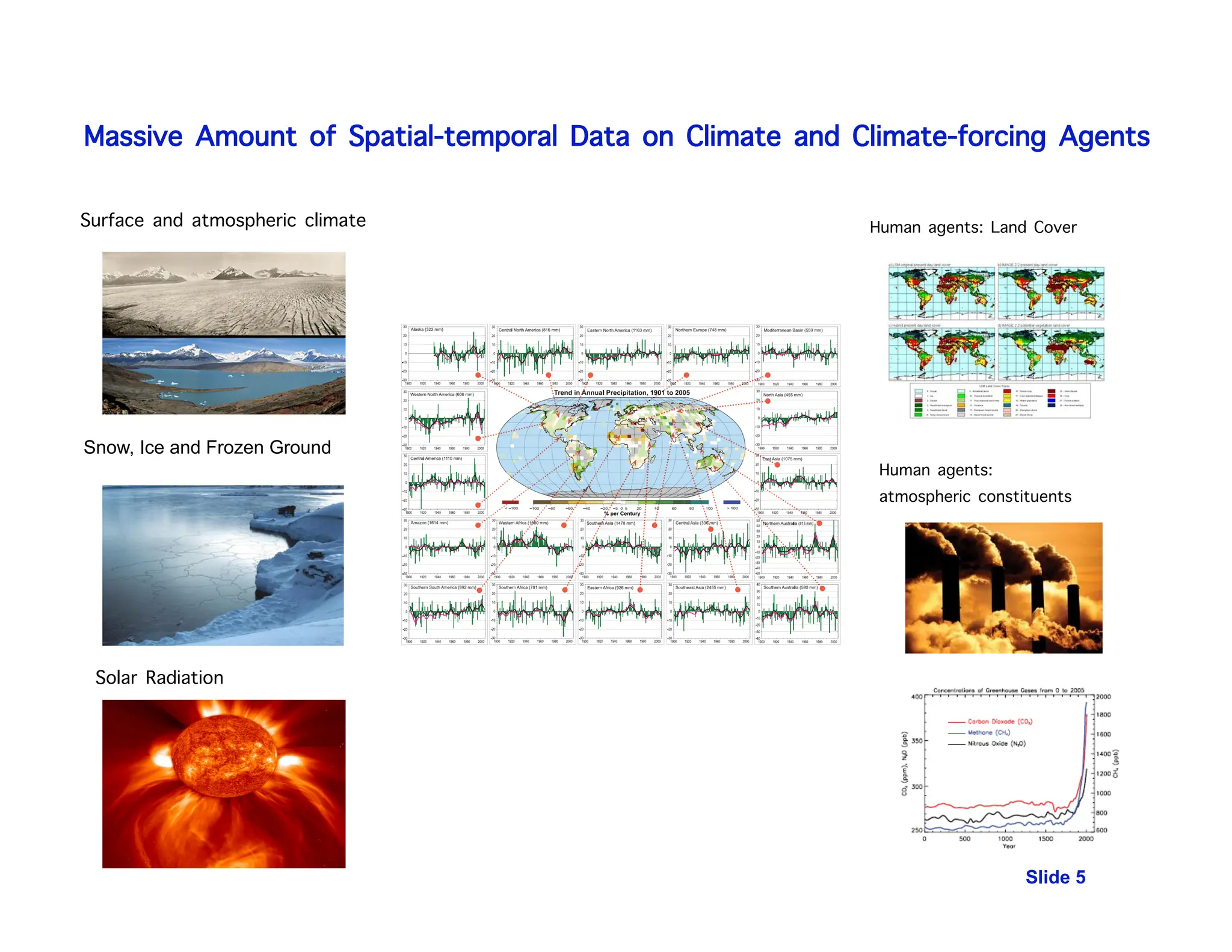
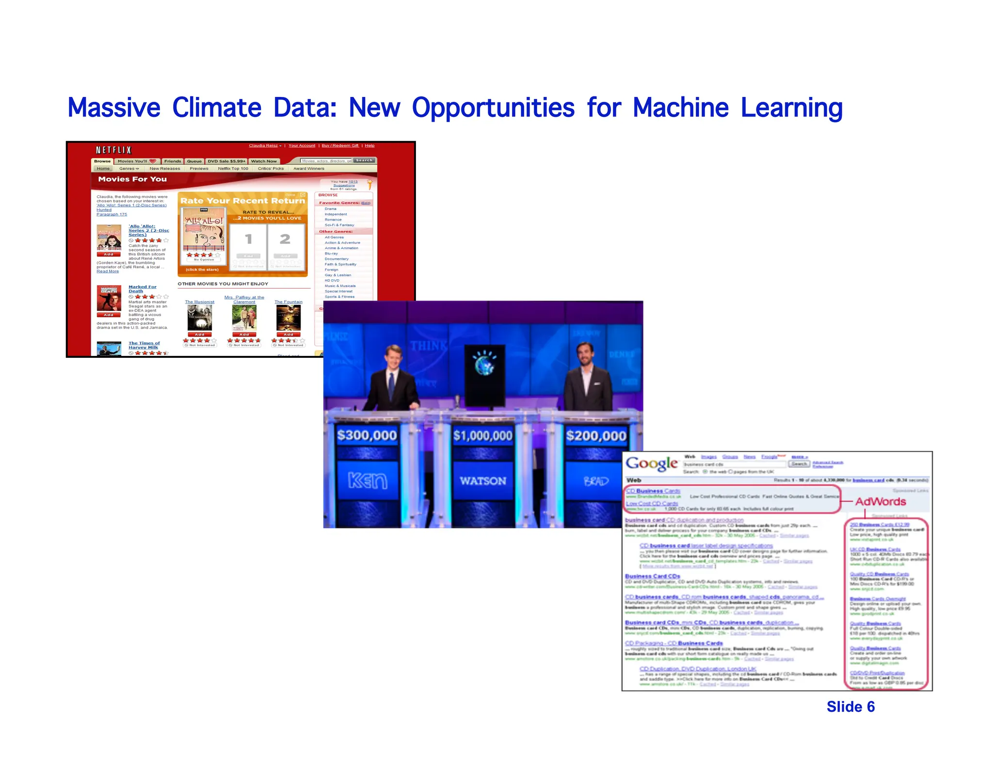
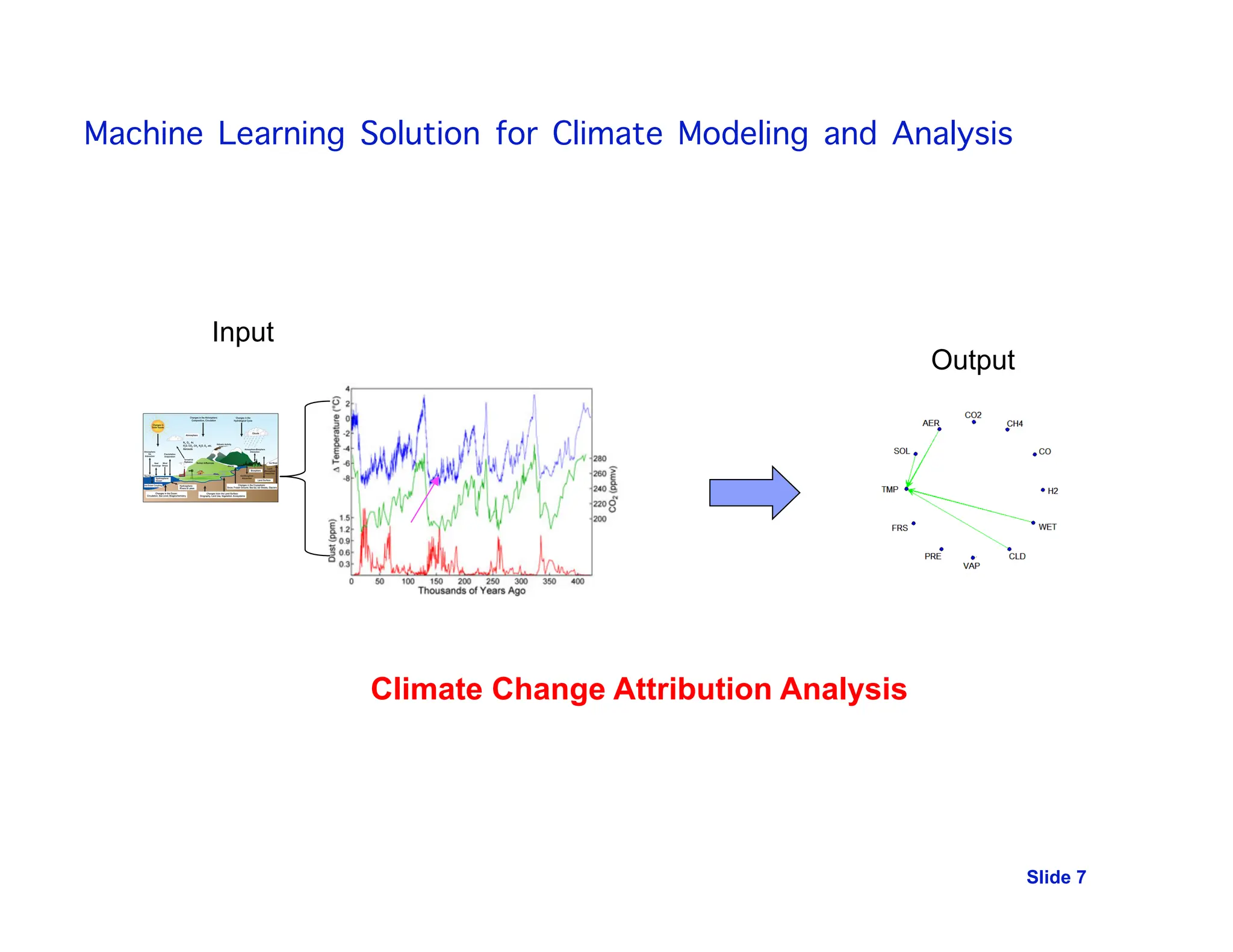
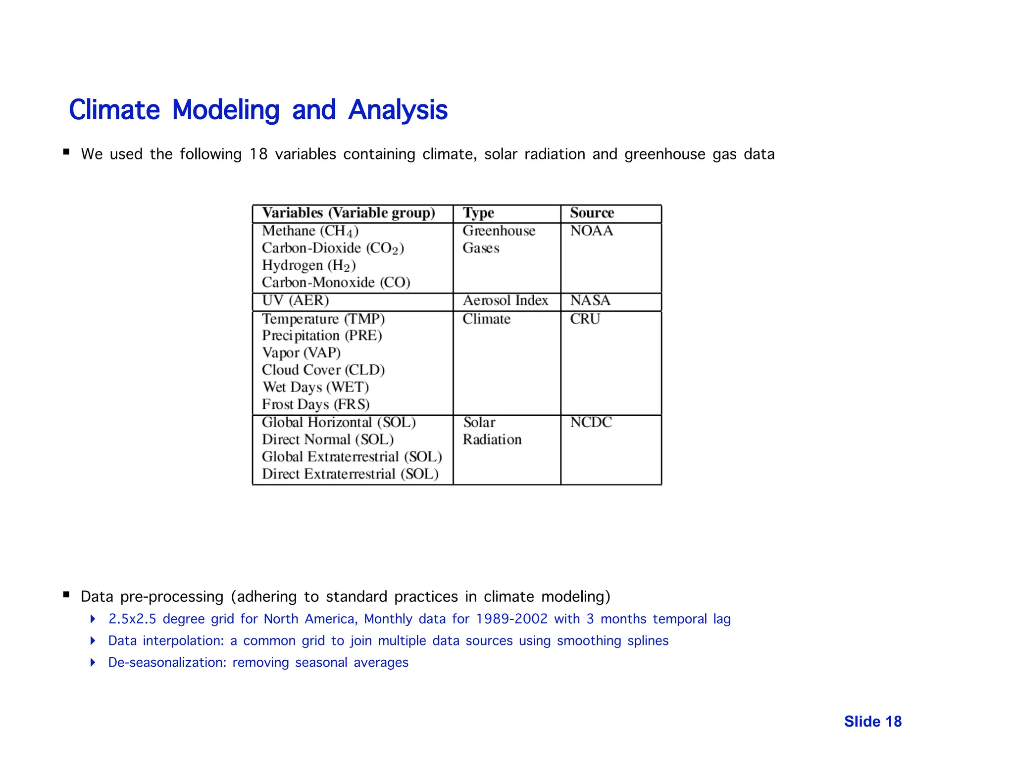
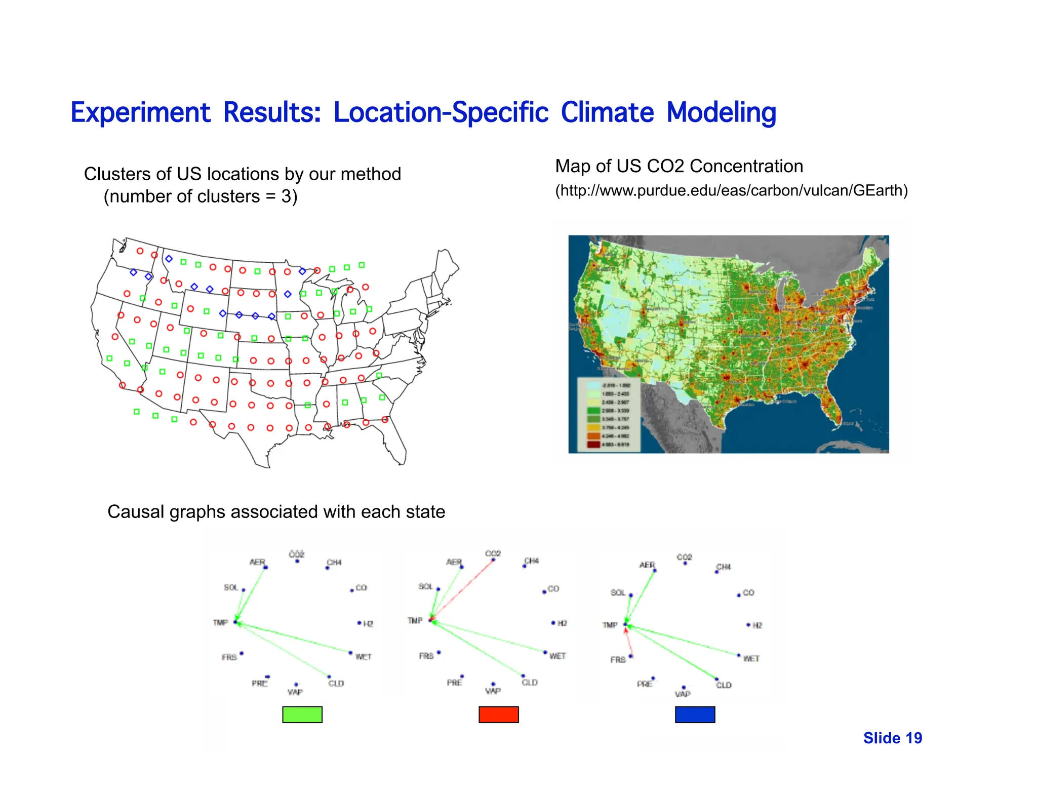
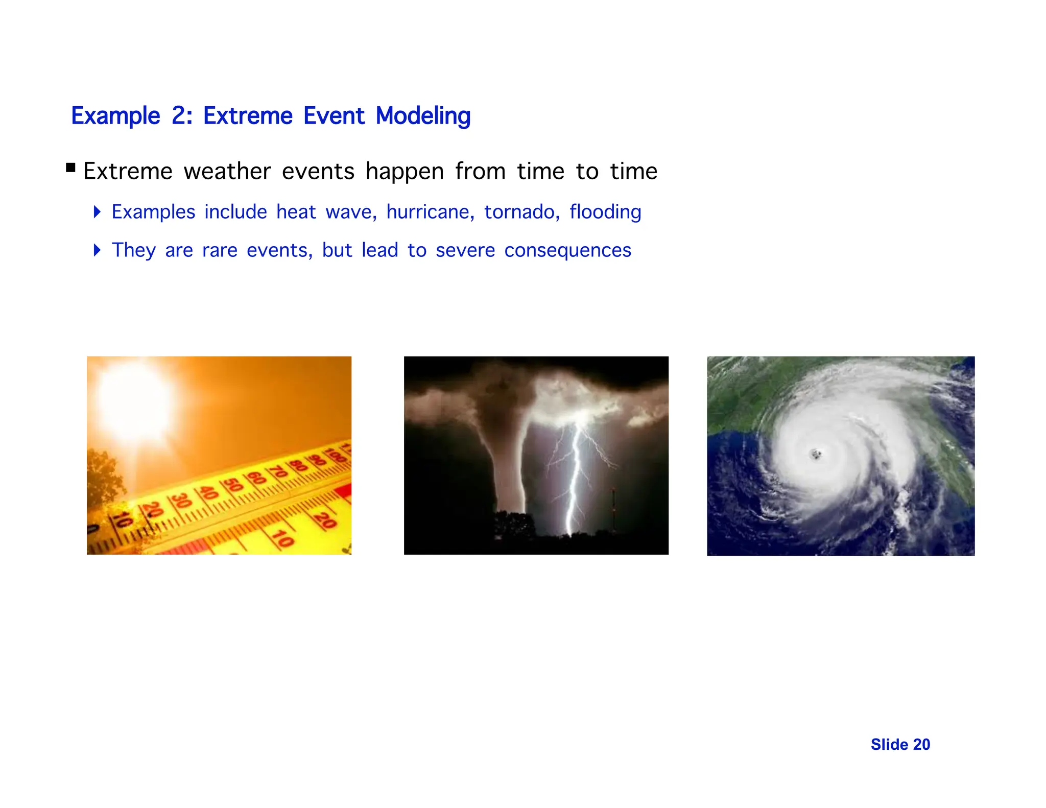
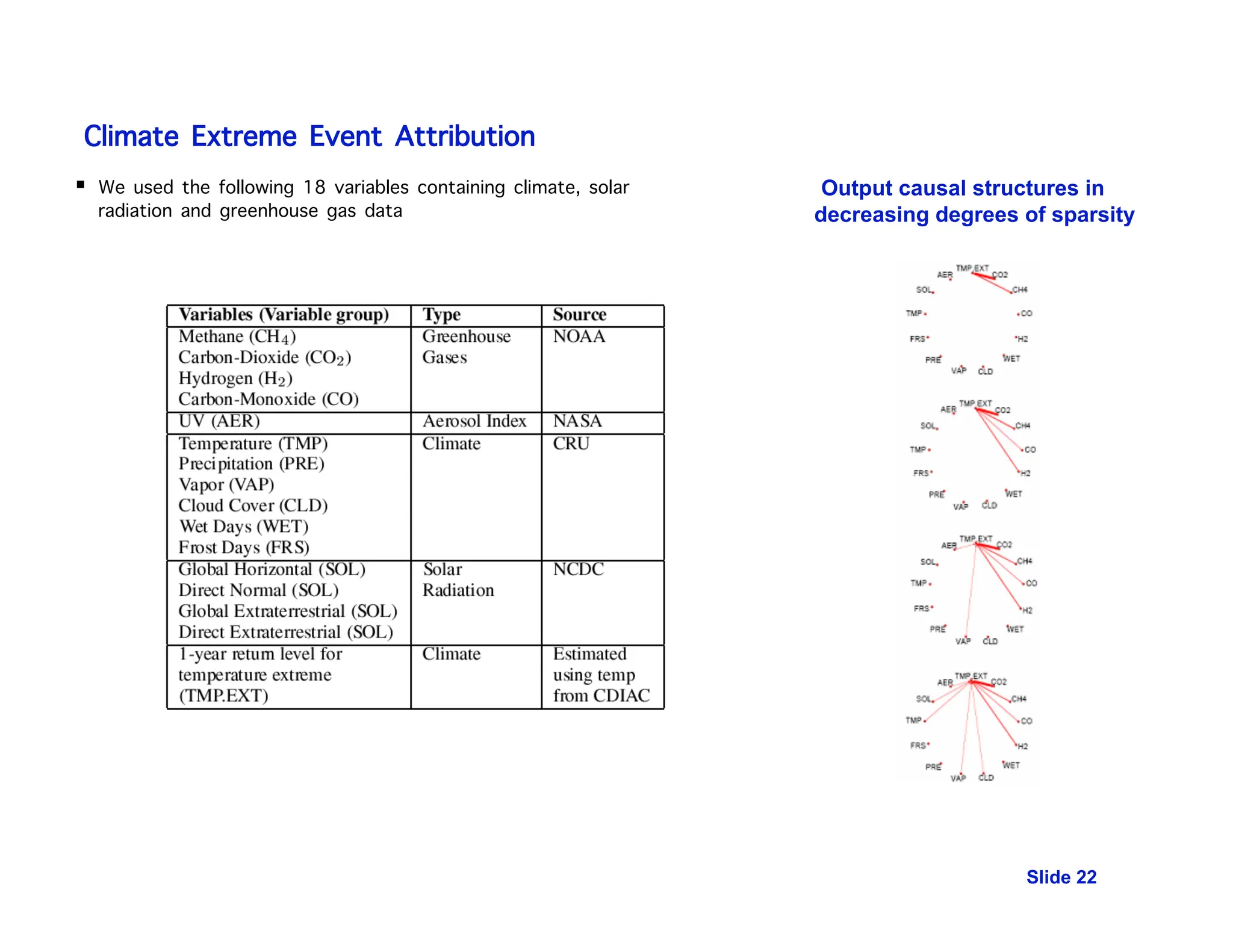
This document discusses the use of temporal causal models, specifically Granger graphical models, for analyzing massive time-series data in climate change attribution and other applications. It highlights the complexity of climate systems and the challenges with existing models, proposing machine learning solutions for better analysis and prediction, including hierarchical Bayesian models for extreme weather events. The research also emphasizes the significance of discovering causal relationships in multivariate time-series data, particularly within the context of gene regulatory networks.

1. 1
Temporal Causal Models for Massive Time-series Data
Mining: Climate Change Attribution and other Applications
Yan Liu
Computer Science Department
Viterbi School of Engineering
University of Southern California
2011 Japan-America Frontiers of Engineering Symposium June 6-8, 2011

2. Climate Change: One of the Most Critical Issues Mankind Faces in the 21st Century
Slide 2

3. Understanding Climate System is Imperative to Devising Potential Solutions
 Climate system involves complex relationships between large number of variables
 Need to understand and quantify “causal” effects of the various parameters
Slide 3

4. Challenges with Existing Climate Models
 23 widely used global climate models: Model inter-
comparison project:
http://www.clivar.org/organization/wgcm/cmip.php
Slide 4
 Forward-simulation approach

5. Massive Amount of Spatial-temporal Data on Climate and Climate-forcing Agents
Slide 5
Human agents:
atmospheric constituents
Surface and atmospheric climate
Snow, Ice and Frozen Ground
Human agents: Land Cover
Solar Radiation

6. Massive Climate Data: New Opportunities for Machine Learning
Slide 6

7. Slide 7
Machine Learning Solution for Climate Modeling and Analysis
Climate Change Attribution Analysis
Input
Output

8. Roadmap
 Introduction of Granger Graphical Models
 Examples of Granger Graphical Models
 Granger Graphical Models for Climate Change Attribution
 Experiment Results on Biology Applications
Slide 8

9. Roadmap
 Introduction of Granger Graphical Models
 Examples of Granger Graphical Models
 Granger Graphical Models for Climate Change Attribution
 Experiment Results on Biology Applications
Slide 9

10. Temporal Causal Modeling by Graphical Granger Modeling Methods
Slide 10
 Our proposed approach for time-series analysis
 Graphical modeling using the notions of Granger causality and methods of variable selection
 Granger causality by the Nobel prize winning economist, Clive Granger
 Definition: a time series x is said to “Granger cause” another time series y, if and only if
regressing for y in terms of both past values of y and x is statically significantly better than
that of regressing in terms of past values of y only
x y

11. Graph Structure Learning
 Graph Structure learning [Heckerman, 1995] has been an active research area
for decades
 Recent progress on L1-penalized regression method for graph structure learning
 LASSO regression for neighborhood selection [Meinshausen and Bühlmann, Ann. Stat. 06]
Consider the p-dimensional multivariate normal distributed random variable:$ $
The neighborhood selection can be solved efficiently with the LASSO
 Block sub-gradient algorithm for finding precision matrix [Banerjee, JMLR 08]
 Efficient fixed-point equations based on a sub-gradient algorithm [Friedman et al.,
Biostatistics 08]
Slide 11

12. Generic Temporal Causal Modeling Method [KDD 2007 joint work with Arnold, Abe]
Slide 12
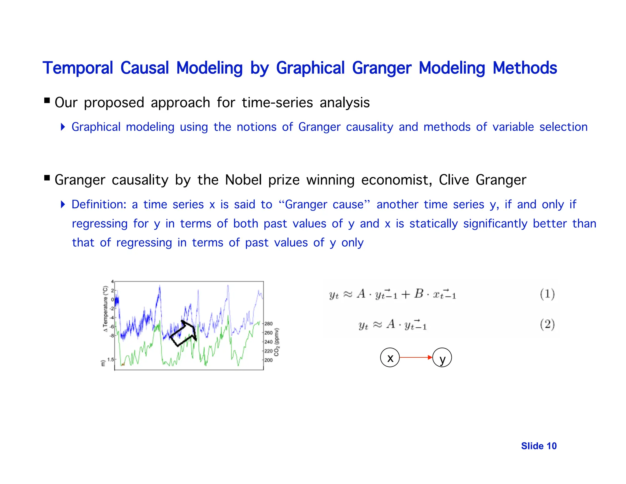
An example of REG can be Lasso [Tibshirani, 1996] Granger Causality
Neighborhood
selection
Structure learning is possible even when the number of variables is
significantly larger than that of the samples

13. Temporal Causal Modeling for Time-series Data Analysis
 Natural grouping of variables
 Group Lasso and group boosting [KDD 2009; ISMB 2009, with Lozano, Abe and Rosset]
 Non-stationary
 Dynamic linear system [KDD 2009, with Kalagnanam and Johnsen]
 Non-linear time-series
 Non-parametric approach [AAAI 2010, with Chen, Liu and Carbonell]
 Spatial time-series
 Spatio-temporal regression via group elastic net [KDD 2009, with Lozano et al.]
 Relational time-series
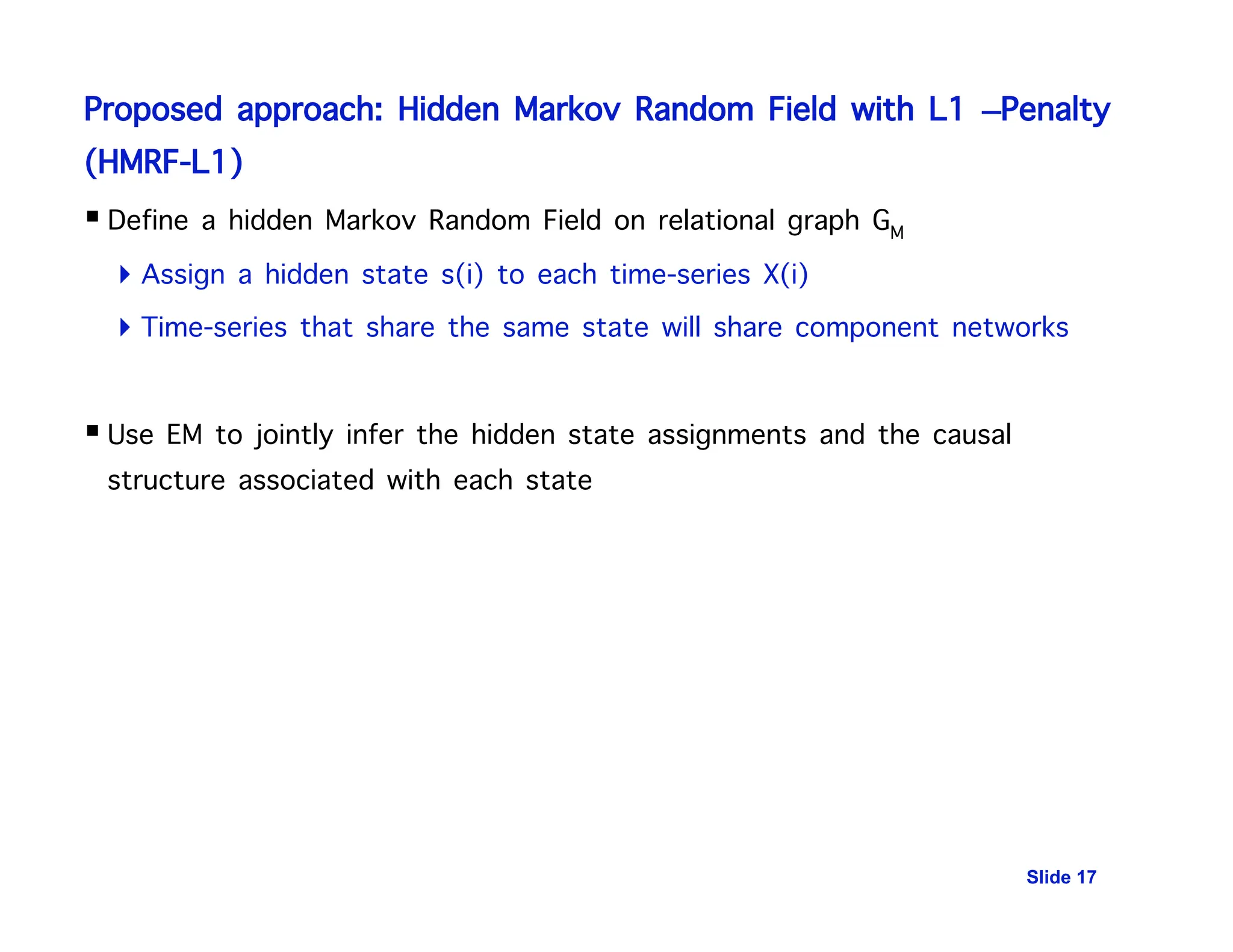
 Hidden Markov random field [Snowbird, ICML 2010, with Niculescu-Mizi, Lozano and Lu]
 Extreme event modeling
 Spatial-temporal extreme value models [KDD 2009, with Lozano et al; NIPS 2011 in
preparation]
Slide 13

14. Roadmap
 Introduction of Granger Graphical Models
 Examples of Granger Graphical Models
 Granger Graphical Models for Climate Change Attribution
 Experiment Results on Biology Applications
Slide 14

15. Slide 15
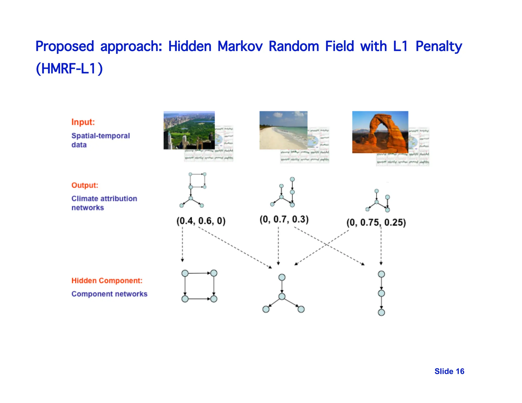
Example 1: Relational Multivariate Time-Series Data [ICML 2010, Liu et al]
 Input: multivariate time-series X(1), …, X(M) and relational graph GM
 Goal: learn a reasonable temporal causal graph for each location/species ..

16. Proposed approach: Hidden Markov Random Field with L1 Penalty
(HMRF-L1)
Slide 16

17. Proposed approach: Hidden Markov Random Field with L1 –Penalty
(HMRF-L1)
Slide 17
 Define a hidden Markov Random Field on relational graph GM
 Assign a hidden state s(i) to each time-series X(i)
 Time-series that share the same state will share component networks
 Use EM to jointly infer the hidden state assignments and the causal
structure associated with each state

18. Slide 18
Climate Modeling and Analysis
 We used the following 18 variables containing climate, solar radiation and greenhouse gas data
 Data pre-processing (adhering to standard practices in climate modeling)
 2.5x2.5 degree grid for North America, Monthly data for 1989-2002 with 3 months temporal lag
 Data interpolation: a common grid to join multiple data sources using smoothing splines
 De-seasonalization: removing seasonal averages

19. Experiment Results: Location-Specific Climate Modeling
Slide 19
Clusters of US locations by our method
(number of clusters = 3)
Causal graphs associated with each state
Map of US CO2 Concentration
(http://www.purdue.edu/eas/carbon/vulcan/GEarth)

20. Slide 20
Example 2: Extreme Event Modeling
 Extreme weather events happen from time to time
 Examples include heat wave, hurricane, tornado, flooding
 They are rare events, but lead to severe consequences

21. Slide 21
Example 2: Extreme Event Modeling
 Key questions to be answered:
 Will the extreme weather happen more intensively?
 Will the extreme weather happen more frequently?
 Our approach: hierarchical Bayesian spatio-temporal dynamic model via extreme
value distribution
 Quantify the stochastic behavior of a process at unusually large or small levels
 A point process incorporating spatio-temporal dependence structures

22. Slide 22
Climate Extreme Event Attribution
 We used the following 18 variables containing climate, solar
radiation and greenhouse gas data
Output causal structures in
decreasing degrees of sparsity

23. Roadmap
 Introduction of Granger Graphical Models
 Examples of Granger Graphical Models
 Granger Graphical Models for Climate Change Attribution
 Experiment Results on Biology Applications
Slide 23

24. Gene Regulatory Network Discovery [ISMB 2010]
Slide 24
Causal graphs discovered by our method
Evaluation against BioGRID
BioGRID
Recent Literature
Precision Recall F1
Our method 0.50 0.72 0.59
Sambo et al. (2008) 0.36 0.44 0.40
 Gene expression regulatory networks for the human cancer cell HeLa S3 [Whitfield
et al., 2002]
 Existing methods in the literature are unable to
 Accommodate lags greater than one
 Handle causality tests involving a large number of genes simultaneously
 Our method addresses both limitations, achieved higher accuracy, and was able
to uncovered previously uncaptured relationships
 CCNA2 to PCNA verified in [Liu, et al 2007]
 CCNE1 to ETF1 verified in [Merdzhanova, et al 2007]
 CCNE1 to CDC6 verified in [Furstenthal, et al 2001]

25. Granger Graphical Models for Time-series Analysis
 A general framework to reveal important dependency information about time-
series data
 Extensions to application data with different properties
 Applications: computational biology, climate science, production management
 Data properties: non-stationary, non-paranormal, relational data, spatial data, natural grouping
 On-going work
 Scalable models to massive data: online algorithms, parallel algorithms
 Anomaly detection and prediction: scalable and interpretable solutions
 Hidden variables: automatically identifying the existence of hidden variables
 Other applications: social-media analysis
Slide 25

26. Acknowledge
 USC Melody Lab
 IBM Research
 Harvard Medical School
Slide 26
Taha Bahadori Yanting Wu Shiv Prakash
Aurelie Lozano Naoki Abe Hongfei Li Alexandru Niculescu-Mizil
Yong Lu