The document describes a data cleaning project to prepare a credit card application dataset for analysis. It involves removing missing values by imputing the mean for continuous variables and mode for categorical variables. The original dataset is from the UCI machine learning repository and contains 690 instances with 15 attributes plus a class attribute. Initial examination found 67 missing values across several attributes. The cleaning process imports the data, analyzes missing values, imputes them, and saves the cleaned dataset for further analysis.


![3 | Page
missing_values = ["?"]
df=pd.read_csv('C:/Users/Owner/Desktop/DATA/CAD/ABC.csv', na_values=missing_values)
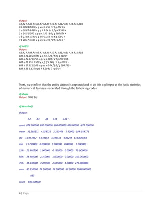
df.isnull().sum()
Output
A1 12
A2 12
A3 0
A4 6
A5 6
A6 9
A7 9
A8 0
A9 0
A10 0
A11 0
A12 0
A13 0
A14 13
A15 0
A16 0
dtype: int64
The total number of missing values is derived using the following code
df.isnull().sum().sum()
Output: 67
To confirm whether or not the dataset was imported correctly, examine the first five (5) and the
last five (5) records of the dataset.
df.head(5)](https://image.slidesharecdn.com/datacleansingproject-190903004809/85/Data-cleansing-project-3-320.jpg)


![10 | Page
z NaN NaN NaN NaN NaN
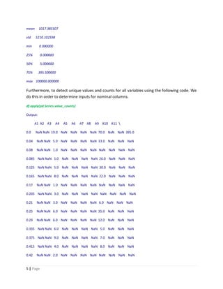
[944 rows x 16 columns]
Step4:
Using the results of step 3 above, the ‘mean’ value will serve as imputes for missing values of
numerical attributes while the ‘mode’ serves as imputes for nominal columns.
Given that the ratio of “missing values to total number of observations is small, between 0.8%
and 1.9%, using the mean and the mode as imputes for missing values is not expected to distort
the dataset in any way.
The following is the code we use to effect these imputations. The seven (7) variables involved
are treated individually.
df['A1'].fillna('b', inplace=True)
df['A2'].fillna(31.568, inplace=True)
df['A4'].fillna('u', inplace=True)
df['A5'].fillna('g', inplace=True)
df['A6'].fillna('c', inplace=True)
df['A7'].fillna('v', inplace=True)
df['A14'].fillna(184, inplace=True)
Step5:
Next, save the clean and new dataset. It is this ‘missing-value free’ dataset that we shall use in
implementing project (all 5 sub-projects) discussed in this portfolio.
df.to_csv('C:/Users/Owner/Desktop/DATA/CAD/ABC-1.csv')
To assess the clean-up exercise, compare the contents of the old and new files for a specific
row / column by using the following codes.
df=pd.read_csv('C:/Users/Owner/Desktop/DATA/CAD/ABC.csv', na_values=missing_values)
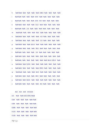
df.iloc[248,:]](https://image.slidesharecdn.com/datacleansingproject-190903004809/85/Data-cleansing-project-10-320.jpg)
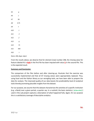
![11 | Page
Output:
A1 NaN
A2 24.5
A3 12.75
A4 u
A5 g
A6 c
A7 bb
A8 4.75
A9 t
A10 t
A11 2
A12 f
A13 g
A14 73
A15 444
A16 +
Name: 248, dtype: object
df=pd.read_csv('C:/Users/Owner/Desktop/DATA/CAD/ABC-1.csv')
df.iloc[248,:]
Output [21]:
Unnamed: 0 248
A1 b
A2 24.5
A3 12.75
A4 u](https://image.slidesharecdn.com/datacleansingproject-190903004809/85/Data-cleansing-project-11-320.jpg)


![제 23회 보아즈(BOAZ) 빅데이터 컨퍼런스 - [MBOAX] : ABSA를 활용한 소비자 반응 분석 기반 운영 효율화 대시보드 설계](https://cdn.slidesharecdn.com/ss_thumbnails/3-1boaz23rdconferencemboax-260203102709-9d519923-thumbnail.jpg?width=640&height=640&fit=bounds)


![7.__Developing_a_Research_Proposal[1].pptx](https://cdn.slidesharecdn.com/ss_thumbnails/7-260131073037-df92dd7d-thumbnail.jpg?width=640&height=640&fit=bounds)


