Data Analytics using SPARK-

1. 19CSH043 – Data Analytics using
SPARK
Optimizing Spark

2. Filter Early, Filter Often
• Big Data is often characterized by a low signal-to noise
ratio.
• Filtering out noise early saves processing cycles, I/O, and
storage in subsequent stages.
• Use filter() transformations to remove unneeded
records and map() transformations to project only
required fields in an RDD.
• Perform these operations before operations that may
invoke a shuffle, such as reduceByKey() or groupByKey().
• Also use them before and after a join() operation.

3. Optimizing Associative Operations
• Associative operations such as sum() and
count() are common requirements when
programming in Spark.
• Often on distributed, partitioned datasets, these
associative key/value operations may involve
shuffling.
• join(), cogroup(), and transformations that have
By or ByKey in their name, such as groupByKey()
or reduceByKey(), can involve shuffling.

4. Optimizing Associative Operations
• shuffle with the ultimate objective of performing an
associative operation—counting occurrences of a key,
for instance —different approaches that can provide
very different performance outcomes.
• difference between using groupByKey() and using
reduceByKey() to perform a sum() or count()
operation.
• group by a key on a partitioned or distributed dataset
solely for the purposes of aggregating values for each
key, using reduceByKey() is generally a better
approach.

5. Optimizing Associative Operations
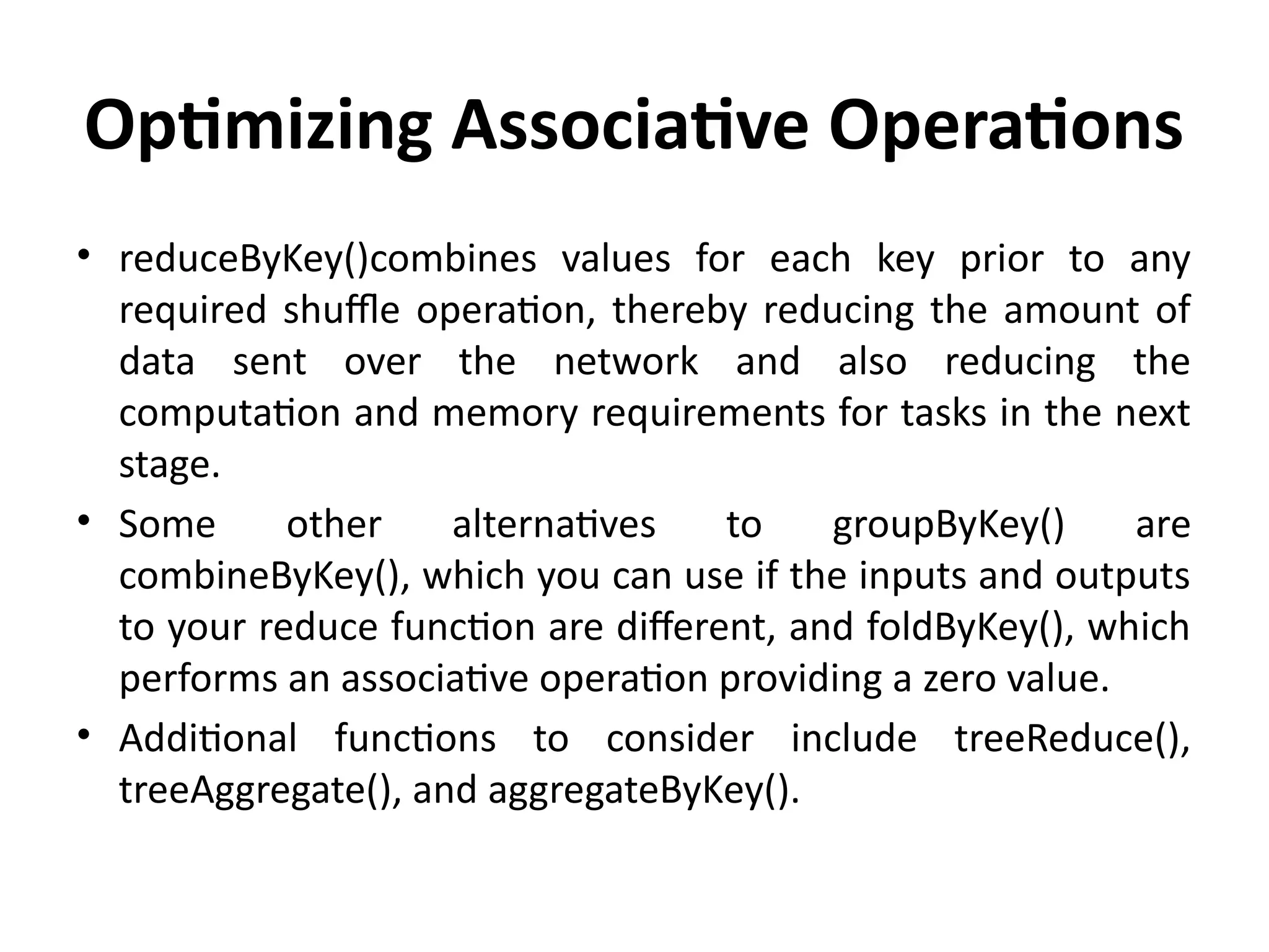
• reduceByKey()combines values for each key prior to any
required shuffle operation, thereby reducing the amount of
data sent over the network and also reducing the
computation and memory requirements for tasks in the next
stage.
• Some other alternatives to groupByKey() are
combineByKey(), which you can use if the inputs and outputs
to your reduce function are different, and foldByKey(), which
performs an associative operation providing a zero value.
• Additional functions to consider include treeReduce(),
treeAggregate(), and aggregateByKey().

6. Understanding the Impact of Functions and
Closures
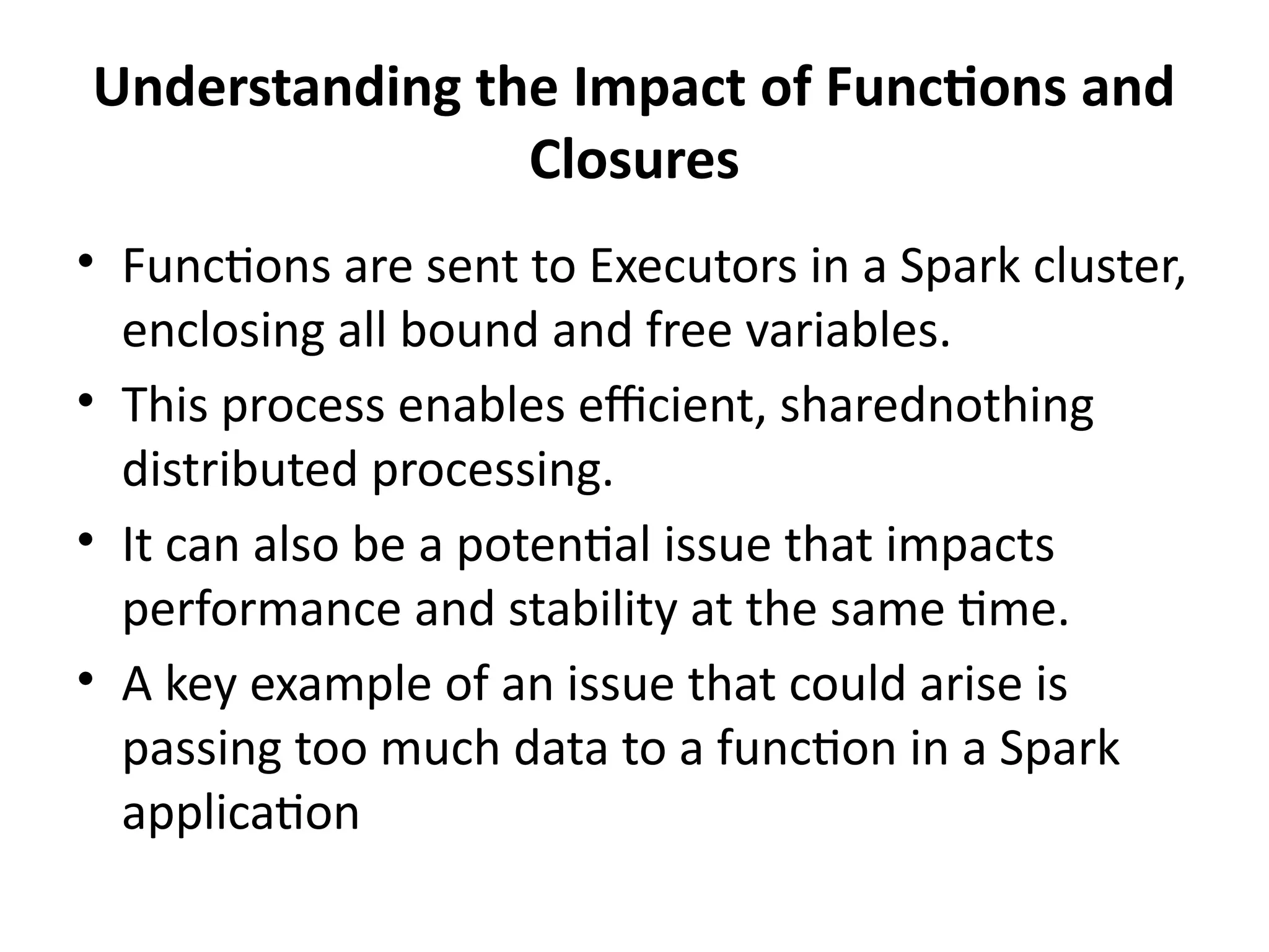
• Functions are sent to Executors in a Spark cluster,
enclosing all bound and free variables.
• This process enables efficient, sharednothing
distributed processing.
• It can also be a potential issue that impacts
performance and stability at the same time.
• A key example of an issue that could arise is
passing too much data to a function in a Spark
application

7. Understanding the Impact of Functions and
Closures
• massive_list = [...]
• def big_fn(x):
• # function enclosing massive_list
• ...
• ...
• rdd.map(lambda x: big_fn(x)).saveAsTextFile...
• # parallelize data which would have otherwise been
enclosed
• massive_list_rdd = sc.parallelize(massive_list)
• rdd.join(massive_list_rdd).saveAsTextFile...

8. Considerations for Collecting Data
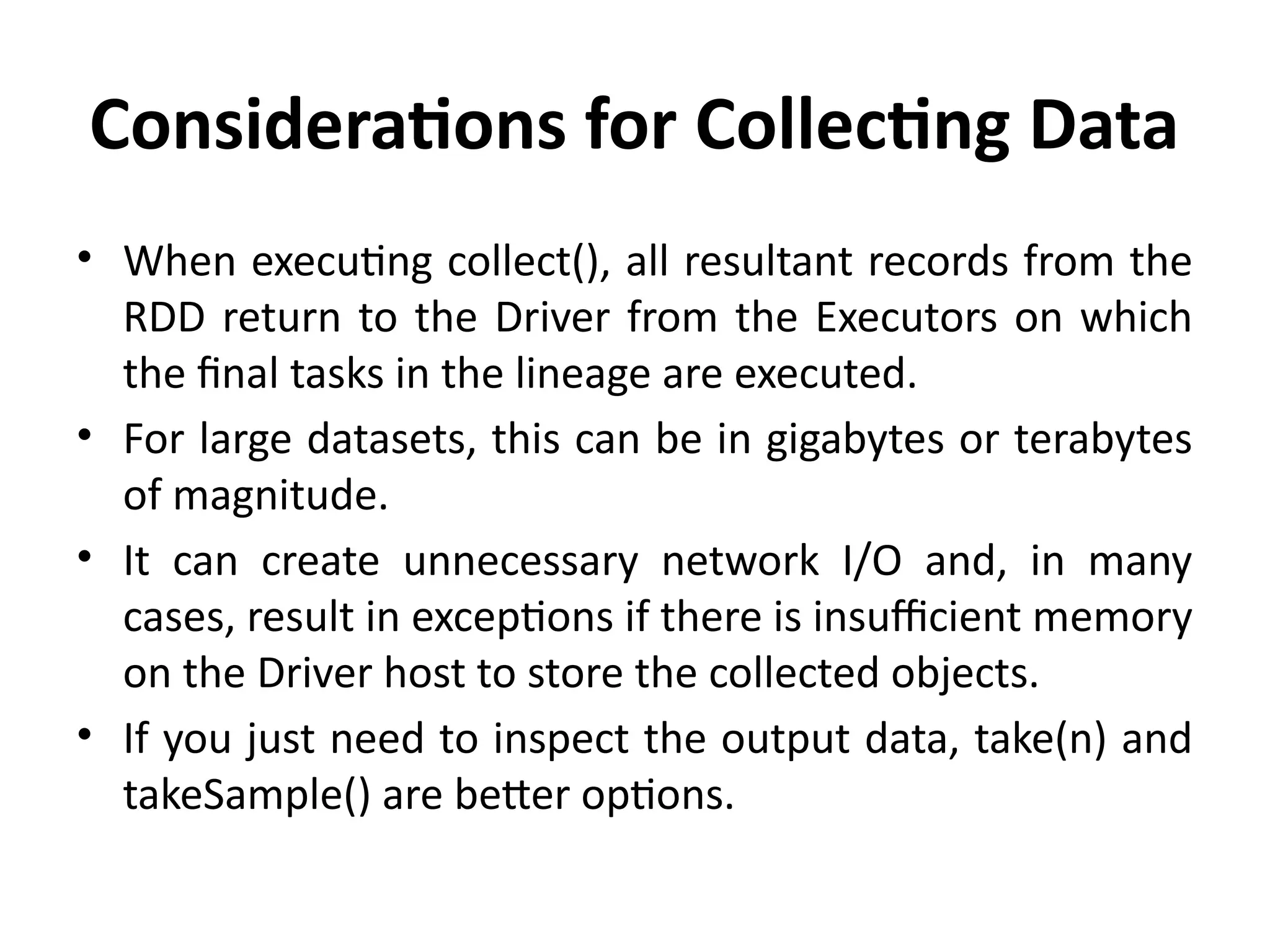
• When executing collect(), all resultant records from the
RDD return to the Driver from the Executors on which
the final tasks in the lineage are executed.
• For large datasets, this can be in gigabytes or terabytes
of magnitude.
• It can create unnecessary network I/O and, in many
cases, result in exceptions if there is insufficient memory
on the Driver host to store the collected objects.
• If you just need to inspect the output data, take(n) and
takeSample() are better options.

9. Configuration Parameters for Tuning and
Optimizing Applications
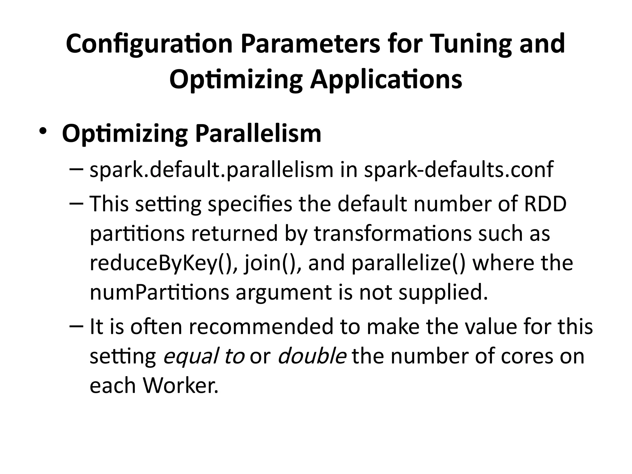
• Optimizing Parallelism
– spark.default.parallelism in spark-defaults.conf
– This setting specifies the default number of RDD
partitions returned by transformations such as
reduceByKey(), join(), and parallelize() where the
numPartitions argument is not supplied.
– It is often recommended to make the value for this
setting equal to or double the number of cores on
each Worker.

10. Configuration Parameters for Tuning and
Optimizing Applications
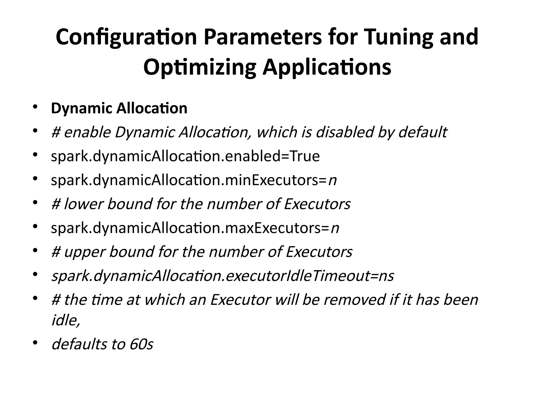
• Dynamic Allocation
• # enable Dynamic Allocation, which is disabled by default
• spark.dynamicAllocation.enabled=True
• spark.dynamicAllocation.minExecutors=n
• # lower bound for the number of Executors
• spark.dynamicAllocation.maxExecutors=n
• # upper bound for the number of Executors
• spark.dynamicAllocation.executorIdleTimeout=ns
• # the time at which an Executor will be removed if it has been
idle,
• defaults to 60s

11. Avoiding Inefficient Partitioning
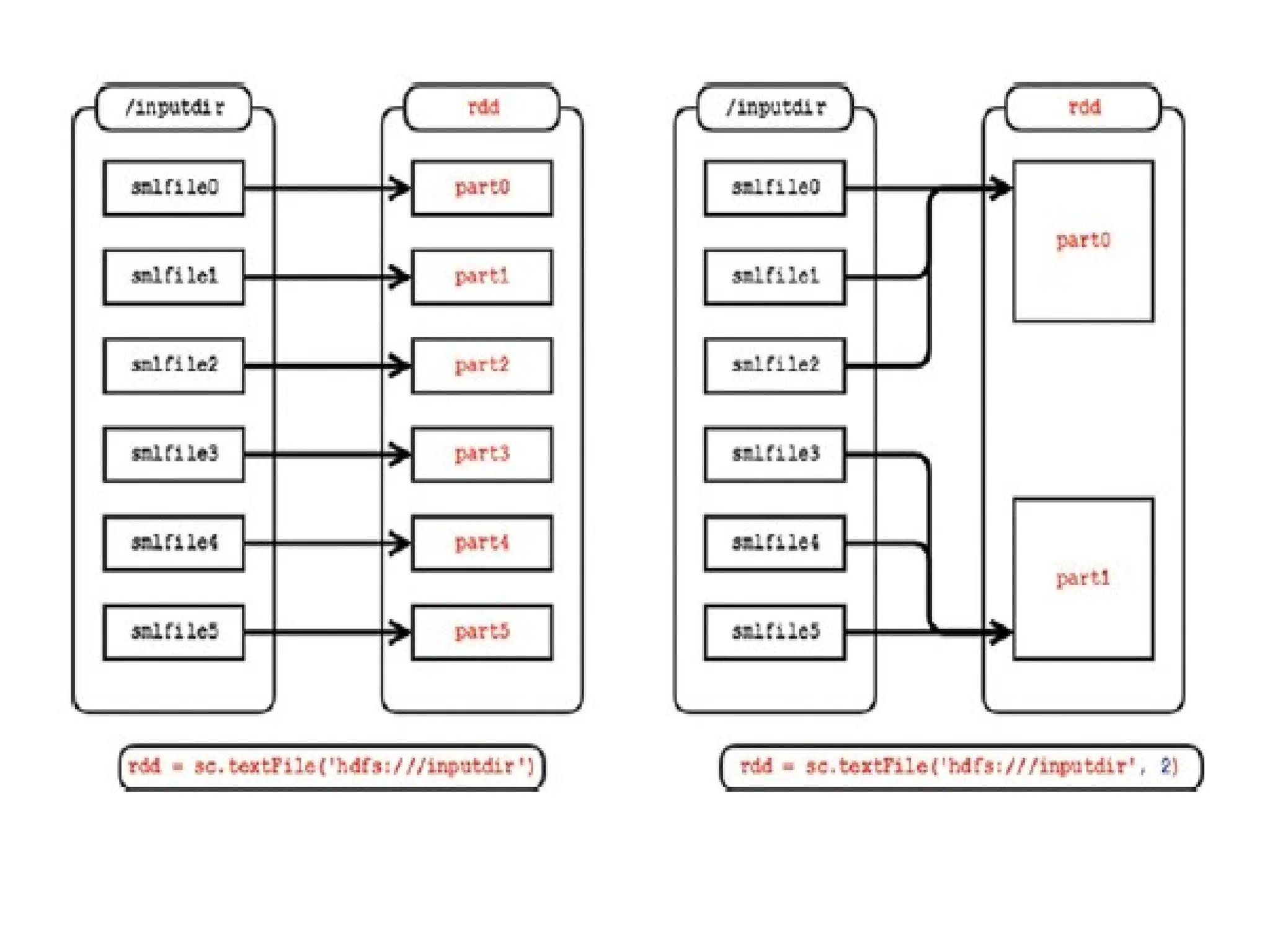
• Small Files Resulting in Too Many Small Partitions
• A filter() operation on a partitioned RDD may result
in some partitions being much smaller than others.
• The solution to this problem is to follow the filter()
operation with a repartition() or coalesce() function
and specify a number less than the input RDD; this
combines small partitions into fewer more
appropriately sized partitions.

13. Avoiding Inefficient Partitioning
• difference between repartition() and coalesce()
is that repartition() always shuffles records if
required,
• whereas coalesce() accepts a shuffle argument
that can be set to False, avoiding a shuffle.
• Therefore, coalesce() can only reduce the
number of partitions, whereas repartition() can
increase or reduce the number of partitions.

14. Avoiding Inefficient Partitioning
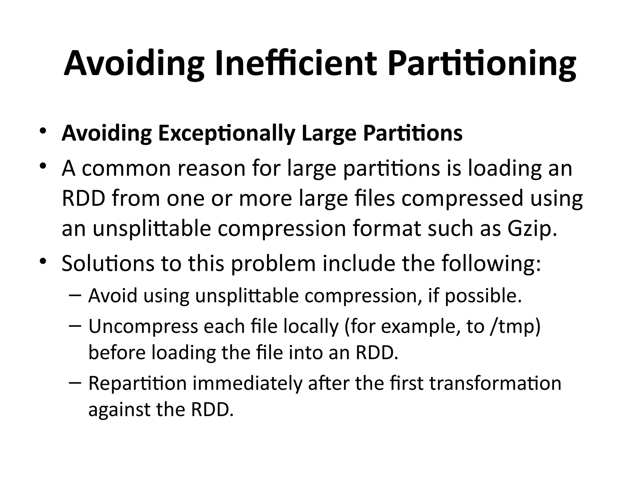
• Avoiding Exceptionally Large Partitions
• A common reason for large partitions is loading an
RDD from one or more large files compressed using
an unsplittable compression format such as Gzip.
• Solutions to this problem include the following:
– Avoid using unsplittable compression, if possible.
– Uncompress each file locally (for example, to /tmp)
before loading the file into an RDD.
– Repartition immediately after the first transformation
against the RDD.

15. Diagnosing Application Performance Issues