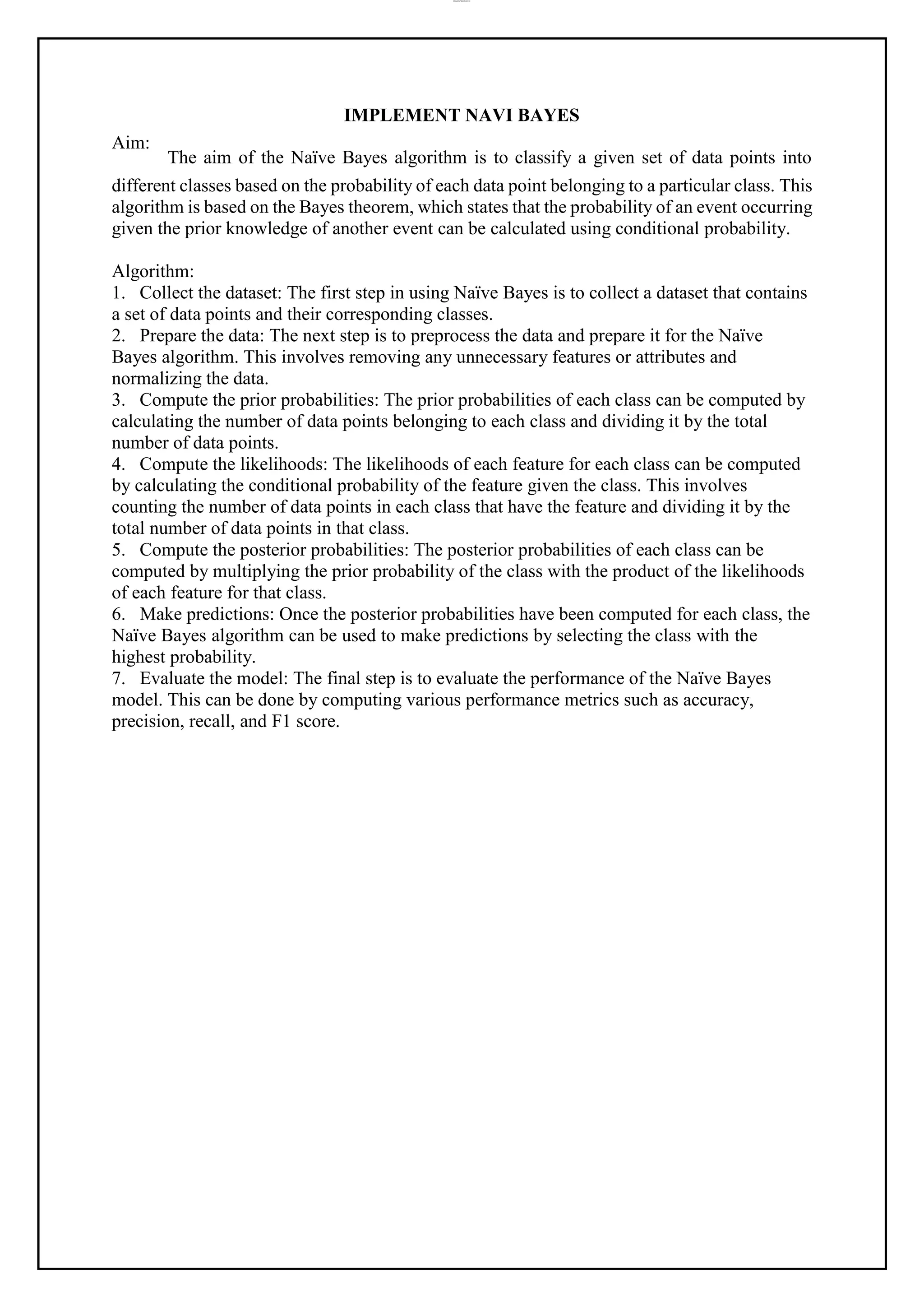
SlideShare a Scribd company logo
1 of 43
lOMoAR cPSD|37458118
CS3941- Artificial Intelligence and Machine Learning
lOMoAR cPSD|37458118
LABORATORY MANUAL
CS 3491 ARTIFICIAL INTELLIGENCE AND MACHINE LEARNING
III Year / VI Semester
REGULATION 2021
lOMoAR cPSD|37458118
COURSE OBJECTIVES:
The main objectives of this course are to:
 Study about uninformed and Heuristic search techniques.
 Learn techniques for reasoning under uncertainty
 Introduce Machine Learning and supervised learning algorithms
 Study about ensembling and unsupervised learning algorithms
 Learn the basics of deep learning using neural networks
PRACTICAL EXERCISES: 30 PERIODS
1. Implementation of Uninformed search algorithms (BFS, DFS)
2. Implementation of Informed search algorithms (A*, memory-bounded A*)
3. Implement naïve Bayes models
4. Implement Bayesian Networks
5. Build Regression models
6. Build decision trees and random forests
7. Build SVM models
8. Implement ensembling techniques
9. Implement clustering algorithms
10. Implement EM for Bayesian networks
11. Build simple NN models
12. Build deep learning NN models
COURSE OUTCOMES: At the end of this course, the students will be able to:
CO1: Use appropriate search algorithms for problem solving
CO2: Apply reasoning under uncertainty
CO3: Build supervised learning models
CO4: Build ensembling and unsupervised models
CO5: Build deep learning neural network models
lOMoAR cPSD|37458118
Aim:
IMPLEMENTING BREADTH-FIRST SEARCH (BFS) AND DEPTH-FIRST
SEARCH (DFS)
The aim of implementing Breadth-First Search (BFS) and Depth-First Search (DFS)
algorithms is to traverse a graph or a tree data structure in a systematic way, visiting all nodes
and edges in the structure in a particular order, without revisiting any node twice.
Algorithm:
Breadth-First Search (BFS) algorithm:
1. Create an empty queue and enqueue the starting node
2. Mark the starting node as visited
3. While the queue is not empty, dequeue a node from the queue and visit it
4. Enqueue all of its neighbors that have not been visited yet, and mark them as visited
5. Repeat steps 3-4 until the queue is empty.
Depth-First Search (DFS) algorithm:
1. Mark the starting node as visited and print it
2. For each adjacent node of the current node that has not been visited, repeat step 1
3. If all adjacent nodes have been visited, backtrack to the previous node and repeat step 2
4. Repeat steps 2-3 until all nodes have been visited
lOMoAR cPSD|37458118
Program:
BFS
graph = {
'5' : ['3','7'],
'3' : ['2', '4'],
'7' : ['8'],
'2' : [],
'4' : ['8'],
'8' : []
}
visited = [] # List for visited nodes.
queue = [] #Initialize a queue
def bfs(visited, graph, node): #function for BFS
visited.append(node)
queue.append(node)
while queue: # Creating loop to visit each node
m = queue.pop(0)
print (m, end = " ")
for neighbour in graph[m]:
if neighbour notin visited:
visited.append(neighbour)
queue.append(neighbour)
# Driver Code
print("Following is the Breadth-First Search")
bfs(visited, graph, '5')
DFS
graph = {
'5' : ['3','7'],
'3' : ['2', '4'],
'7' : ['8'],
'2' : [],
'4' : ['8'],
'8' : []
}
visited = set() # Set to keep track of visited nodes of graph.
lOMoAR cPSD|37458118
defdfs(visited, graph, node): #function for dfs
if node not in visited:
print (node)
visited.add(node)
for neighbour in graph[node]:
dfs(visited, graph, neighbour)
# Driver Code
print("Following is the Depth-First Search")
dfs(visited, graph, '5')
lOMoAR cPSD|37458118
Output:
BFS
Following is the Breadth-First Search
5 3 7 2 4 8
DFS
Following is the Depth-First Search
5
3
2
4
8
7
Result:
Thus the program for BFS and DFS is executed successfully and output is verified.
lOMoAR cPSD|37458118
Aim:
IMPLEMENTING INFORMED SEARCH ALGORITHMS LIKE A* AND
MEMORY-BOUNDED A*
The aim of a C program for implementing informed search algorithms like A* and
memory-bounded A* is to efficiently find the shortest path between two points in a graph or
network. The A* algorithm is a heuristic-based search algorithm that finds the shortest path
between two points by evaluating the cost function of each possible path. The memory-
bounded A* algorithm is a variant of the A* algorithm that uses a limited amount of memory
and is suitable for large search spaces.
Algorithm:
Algorithm for A*
1. Initialize the starting node with a cost of zero and add it to an open list.
2. While the open list is not empty:
a. Find the node with the lowest cost in the open list and remove it.
b. If this node is the goal node, return the path to this node.
c. Generate all successor nodes of the current node.
d. For each successor node, calculate its cost and add it to the open list.
3. If the open list is empty and the goal node has not been found, then there is no path from
the start node to the goal node.
Algorithm for memory-bounded A*
1. Initialize the starting node with a cost of zero and add it to an open list and a closed list.
2. While the open list is not empty:
a. Find the node with the lowest cost in the open list and remove it.
b. If this node is the goal node, return the path to this node.
c. Generate all successor nodes of the current node.
d. For each successor node, calculate its cost and add it to the open list if it is not in the
closed list. e. If the open list is too large, remove the node with the highest cost from the open
list and add it to the closed list.
f. Add the current node to the closed list.
3. If the open list is empty and the goal node has not been found, then there is no path from
the start node to the goal node.
lOMoAR cPSD|37458118
Program:
from queue importPriorityQueue
v =14
graph =[[] fori inrange(v)]
# Function For Implementing Best First Search
# Gives output path having lowest cost
defbest_first_search(actual_Src, target, n):
visited =[False] *n
pq =PriorityQueue()
pq.put((0, actual_Src))
visited[actual_Src] =True
whilepq.empty() ==False:
u =pq.get()[1]
# Displaying the path having lowest cost
print(u, end=" ")
ifu ==target:
break
forv, c ingraph[u]:
ifvisited[v] ==False:
visited[v] =True
pq.put((c, v))
print()
# Function for adding edges to graph
defaddedge(x, y, cost):
graph[x].append((y, cost))
graph[y].append((x, cost))
# The nodes shown in above example(by alphabets) are
# implemented using integers addedge(x,y,cost);
addedge(0, 1, 3)
addedge(0, 2, 6)
addedge(0, 3, 5)
addedge(1, 4, 9)
addedge(1, 5, 8)
addedge(2, 6, 12)
addedge(2, 7, 14)
addedge(3, 8, 7)
addedge(8, 9, 5)
addedge(8, 10, 6)
addedge(9, 11, 1)
addedge(9, 12, 10)
addedge(9, 13, 2)
source =0
target =9
best_first_search(source, target, v)
lOMoAR cPSD|37458118
Memory bounded A*
import numpy as np
import heapq
class Graph:
def __init__(self, adjacency_matrix):
self.adjacency_matrix = adjacency_matrix
self.num_nodes = len(adjacency_matrix)
def get_neighbors(self, node):
return [neighbor for neighbor, is_connected in enumerate(self.adjacency_matrix[node]) if is_connected]
def memory_bounded_a_star(graph, start, goal, memory_limit):
visited = set()
priority_queue = [(0, start)]
memory_usage = 0
while priority_queue:
memory_usage = max(memory_usage, len(visited))
if memory_usage > memory_limit:
print("Memory limit exceeded!")
return None
cost, current_node = heapq.heappop(priority_queue)
if current_node == goal:
print("Goal found!")
return cost
if current_node not in visited:
visited.add(current_node)
for neighbor in graph.get_neighbors(current_node):
heapq.heappush(priority_queue, (cost + 1, neighbor))
print("Goal not reachable!")
return None
if __name__ == "__main__":
# Define the adjacency matrix of the graph
adjacency_matrix = np.array([
[0, 1, 1, 0, 0, 0, 0],
[1, 0, 0, 1, 1, 0, 0],
[1, 0, 0, 0, 0, 1, 0],
[0, 1, 0, 0, 0, 1, 1],
[0, 1, 0, 0, 0, 0, 1],
[0, 0, 1, 1, 0, 0, 1],
[0, 0, 0, 1, 1, 1, 0]
])
graph = Graph(adjacency_matrix)
start_node = 0
goal_node = 6
memory_limit = 10 # Set the memory limit
result = memory_bounded_a_star(graph, start_node, goal_node, memory_limit)
print("Shortest path cost:", result)
lOMoAR cPSD|37458118
Output:
A*
0 1 3 2 8 9
Memory Bounded A*
Goal found!
Shortest path cost: 3
Result:
Thus the program for implementing informed search algorithms like A* and memory-
bounded A* has verified successfully and output is verified.
lOMoAR cPSD|37458118
Aim:
IMPLEMENT NAVI BAYES
The aim of the Naïve Bayes algorithm is to classify a given set of data points into
different classes based on the probability of each data point belonging to a particular class. This
algorithm is based on the Bayes theorem, which states that the probability of an event occurring
given the prior knowledge of another event can be calculated using conditional probability.
Algorithm:
1. Collect the dataset: The first step in using Naïve Bayes is to collect a dataset that contains
a set of data points and their corresponding classes.
2. Prepare the data: The next step is to preprocess the data and prepare it for the Naïve
Bayes algorithm. This involves removing any unnecessary features or attributes and
normalizing the data.
3. Compute the prior probabilities: The prior probabilities of each class can be computed by
calculating the number of data points belonging to each class and dividing it by the total
number of data points.
4. Compute the likelihoods: The likelihoods of each feature for each class can be computed
by calculating the conditional probability of the feature given the class. This involves
counting the number of data points in each class that have the feature and dividing it by the
total number of data points in that class.
5. Compute the posterior probabilities: The posterior probabilities of each class can be
computed by multiplying the prior probability of the class with the product of the likelihoods
of each feature for that class.
6. Make predictions: Once the posterior probabilities have been computed for each class, the
Naïve Bayes algorithm can be used to make predictions by selecting the class with the
highest probability.
7. Evaluate the model: The final step is to evaluate the performance of the Naïve Bayes
model. This can be done by computing various performance metrics such as accuracy,
precision, recall, and F1 score.
lOMoAR cPSD|37458118
Program:
# Importing library
import math
import random
import csv
# the categorical class names are changed to numeric data
# eg: yes and no encoded to 1 and 0 def
encode_class(mydata):
classes = []
for i in range(len(mydata)):
ifmydata[i][-1] not in classes:
classes.append(mydata[i][-1])
for i in range(len(classes)):
for j in range(len(mydata)):
if mydata[j][-1] == classes[i]:
mydata[j][-1] = i
return mydata
# Splitting the data
def splitting(mydata, ratio):
train_num = int(len(mydata) * ratio)
train = []
# initiallytestset will have all the dataset
test = list(mydata)
whilelen(train) <train_num:
# index generated randomly from range 0
# to length of testset
index = random.randrange(len(test))
# from testset, pop data rows and put it in train
train.append(test.pop(index))
return train, test
# Group the data rows under each class yes or
# no in dictionary eg: dict[yes] and dict[no]
defgroupUnderClass(mydata):
dict = {}
for i in range(len(mydata)):
if (mydata[i][-1] not in dict):
dict[mydata[i][-1]] = []
dict[mydata[i][-1]].append(mydata[i])
returndict
# Calculating Mean
def mean(numbers):
return sum(numbers) / float(len(numbers))
# Calculating Standard Deviation
lOMoAR cPSD|37458118
defstd_dev(numbers):
avg = mean(numbers)
variance = sum([pow(x - avg, 2) for x in numbers]) / float(len(numbers) - 1)
returnmath.sqrt(variance)
defMeanAndStdDev(mydata):
info = [(mean(attribute), std_dev(attribute)) for attribute in zip(*mydata)]
# eg: list = [ [a, b, c], [m, n, o], [x, y, z]]
# here mean of 1st attribute =(a + m+x), mean of 2nd attribute = (b + n+y)/3
# delete summaries of last class
del info[-1]
return info
# find Mean and Standard Deviation under each class
defMeanAndStdDevForClass(mydata):
info = {}
dict = groupUnderClass(mydata)
forclassValue, instances in dict.items():
info[classValue] = MeanAndStdDev(instances)
return info
# Calculate Gaussian Probability Density Function
defcalculateGaussianProbability(x, mean, stdev):
expo = math.exp(-(math.pow(x - mean, 2) / (2 * math.pow(stdev, 2))))
return (1 / (math.sqrt(2 * math.pi) * stdev)) * expo
# Calculate Class Probabilities
defcalculateClassProbabilities(info, test):
probabilities = {}
forclassValue, classSummaries in info.items():
probabilities[classValue] = 1
for i in range(len(classSummaries)):
mean, std_dev = classSummaries[i]
x = test[i]
probabilities[classValue] *= calculateGaussianProbability(x, mean,
std_dev)
return probabilities
# Make prediction - highest probability is the prediction
def predict(info, test):
probabilities = calculateClassProbabilities(info, test)
bestLabel, bestProb = None, -1
forclassValue, probability in probabilities.items():
ifbestLabel is None or probability >bestProb:
bestProb = probability
bestLabel = classValue
returnbestLabel
lOMoAR cPSD|37458118
# returns predictions for a set of examples
defgetPredictions(info, test):
predictions = []
for i in range(len(test)):
result = predict(info, test[i])
predictions.append(result)
return predictions
# Accuracy score
defaccuracy_rate(test, predictions):
correct = 0
for i in range(len(test)):
if test[i][-1] == predictions[i]:
correct += 1
return (correct / float(len(test))) * 100.0
# driver code
# add the data path in your system
filename = r'E:userMACHINE LEARNINGmachine learning algosNaive
bayesfiledata.csv'
# load the file and store it in mydata list
mydata = csv.reader(open(filename, "rt"))
mydata = list(mydata)
mydata = encode_class(mydata)
for i in range(len(mydata)):
mydata[i] = [float(x) for x in mydata[i]]
# split ratio = 0.7
# 70% of data is training data and 30% is test data used for testing
ratio = 0.7
train_data, test_data = splitting(mydata, ratio)
print('Total number of examples are: ', len(mydata))
print('Out of these, training examples are: ', len(train_data))
print("Test examples are: ", len(test_data))
# prepare model
info = MeanAndStdDevForClass(train_data)
# test model
predictions = getPredictions(info, test_data)
accuracy = accuracy_rate(test_data, predictions)
print("Accuracy of your model is: ", accuracy)
lOMoAR cPSD|37458118
Output:
Total number of examples are: 200
Out of these, training examples are: 140
Test examples are: 60
Accuracy of your model is: 71.2376788
Result:
Thus the program for Navy Bayes is verified successfully and output is verified.
lOMoAR cPSD|37458118
Aim:
IMPLEMENT BAYESIAN NETWORKS
The aim of implementing Bayesian Networks is to model the probabilistic
relationships between a set of variables. A Bayesian Network is a graphical model that
represents the conditional dependencies between different variables in a probabilistic manner.
It is a powerful tool for reasoning under uncertainty and can be used for a wide range of
applications, including decision making, risk analysis, and prediction.
Algorithm:
1. Define the variables: The first step in implementing a Bayesian Network is to define the
variables that will be used in the model. Each variable should be clearly defined and its
possible states should be enumerated.
2. Determine the relationships between variables: The next step is to determine the
probabilistic relationships between the variables. This can be done by identifying the causal
relationships between the variables or by using data to estimate the conditional probabilities
of each variable given its parents.
3. Construct the Bayesian Network: The Bayesian Network can be constructed by
representing the variables as nodes in a directed acyclic graph (DAG). The edges between the
nodes represent the conditional dependencies between the variables.
4. Assign probabilities to the variables: Once the structure of the Bayesian Network has
been defined, the probabilities of each variable must be assigned. This can be done by using
expert knowledge, data, or a combination of both.
5. Inference: Inference refers to the process of using the Bayesian Network to make
predictions or draw conclusions. This can be done by using various inference algorithms,
such as variable elimination or belief propagation.
6. Learning: Learning refers to the process of updating the probabilities in the Bayesian
Network based on new data. This can be done using various learning algorithms, such as
maximum likelihood or Bayesian learning.
7. Evaluation: The final step in implementing a Bayesian Network is to evaluate its
performance. This can be done by comparing the predictions of the model to actual data and
computing various performance metrics, such as accuracy or precision.
lOMoAR cPSD|37458118
Program:
Import numpy as np
import csv
import pandas as pd
from pgmpy.models import BayesianModel
from pgmpy.estimators import MaximumLikelihoodEstimator
from pgmpy.inference import VariableElimination
#read Cleveland Heart Disease data
heartDisease = pd.read_csv('heart.csv')
heartDisease = heartDisease.replace('?',np.nan)
#display the data
print('Few examples from the dataset are given below')
print(heartDisease.head())
#Model Bayesian Network
Model=BayesianModel([('age','trestbps'),('age','fbs'),
('sex','trestbps'),('exang','trestbps'),('trestbps','heartdise
ase'),('fbs','heartdisease'),('heartdisease','restecg'),
('heartdisease','thalach'),('heartdisease','chol')])
#Learning CPDs using Maximum Likelihood Estimators
print('n Learning CPD using Maximum likelihood estimators')
model.fit(heartDisease,estimator=MaximumLikelihoodEstimator)
# Inferencing with Bayesian Network
print('n Inferencing with Bayesian Network:')
HeartDisease_infer = VariableElimination(model)
#computing the Probability of HeartDisease given Age
print('n 1. Probability of HeartDisease given Age=30')
q=HeartDisease_infer.query(variables=['heartdisease'],evidence
={'age':28})
print(q['heartdisease'])
#computing the Probability of HeartDisease given cholesterol
print('n 2. Probability of HeartDisease given cholesterol=100')
q=HeartDisease_infer.query(variables=['heartdisease'],evidence
={'chol':100})
print(q['heartdisease'])
lOMoAR cPSD|37458118
Output:
age sex cptrestbps ...slope cathalheartdisease
0 63 1 1 145 ... 3 0 6 0
1 67 1 4 160 ... 2 3 3 2
2 67 1 4 120 ... 2 2 7 1
3 37 1 3 130 ... 3 0 3 0
4 41 0 2 130 ... 1 0 3 0
[5 rows x 14 columns]
Learning CPD using Maximum likelihood estimators
Inferencing with Bayesian Network:
1. Probability of HeartDisease given Age=28
╒════════════════╤═════════════════════╕
│ heartdisease │ phi(heartdisease) │
╞════════════════╪═════════════════════╡
│ heartdisease_0 │ 0.6791 │
├────────────────┼─────────────────────┤
│ heartdisease_1 │ 0.1212 │
├────────────────┼─────────────────────┤
│ heartdisease_2 │ 0.0810 │
├────────────────┼─────────────────────┤
│ heartdisease_3 │ 0.0939 │
├────────────────┼─────────────────────┤
│ heartdisease_4 │ 0.0247 │
╘════════════════╧═════════════════════╛
2. Probability of HeartDisease given cholesterol=100
╒════════════════╤═════════════════════╕
│ heartdisease │ phi(heartdisease) │
╞════════════════╪═════════════════════╡
│ heartdisease_0 │ 0.5400 │
├────────────────┼─────────────────────┤
│ heartdisease_1 │ 0.1533 │
├────────────────┼─────────────────────┤
│ heartdisease_2 │ 0.1303 │
├────────────────┼─────────────────────┤
│ heartdisease_3 │ 0.1259 │
├────────────────┼─────────────────────┤
│ heartdisease_4 │ 0.0506 │
╘════════════════╧═════════════════════╛
Result:
Thus the program is executed successfully and output is verified.
lOMoAR cPSD|37458118
Aim:
BUILD REGRESSION MODEL
The aim of building a regression model is to predict a continuous numerical outcome
variable based on one or more input variables. There are several algorithms that can be used
to build regression models, including linear regression, polynomial regression, decision trees,
random forests, and neural networks.
Algorithm:
1. Collecting and cleaning the data: The first step in building a regression model is to gather
the data needed for analysis and ensure that it is clean and consistent. This may involve
removing missing values, outliers, and other errors.
2. Exploring the data: Once the data is cleaned, it is important to explore it to gain an
understanding of the relationships between the input and outcome variables. This may involve
calculating summary statistics, creating visualizations, and testing for correlations.
3. Choosing the algorithm: Based on the nature of the problem and the characteristics of the
data, an appropriate regression algorithm is chosen.
4. Preprocessing the data: Before applying the regression algorithm, it may be necessary to
preprocess the data to ensure that it is in a suitable format. This may involve standardizing or
normalizing the data, encoding categorical variables, or applying feature engineering
techniques.
5. Training the model: The regression model is trained on a subset of the data, using an
optimization algorithm to find the values of the model parameters that minimize the difference
between the predicted and actual values.
6. Evaluating the model: Once the model is trained, it is evaluated using a separate test dataset
to determine its accuracy and generalization performance. Metrics such as mean squared error,
R-squared, or root mean squared error can be used to assess the model's performance.
7. Improving the model: Based on the evaluation results, the model can be refined by adjusting
the model parameters or using different algorithms.
8. Deploying the model: Finally, the model can be deployed to make predictions on new data.
lOMoAR cPSD|37458118
Program:
import pandas as pd
importnumpy as np
importmatplotlib.pyplot as plt
fromsklearn.linear_model import LinearRegression
fromsklearn.model_selection import train_test_split
fromsklearn.metrics import mean_squared_error, r2_score
# Load the dataset
df = pd.read_csv('dataset.csv')
# Split the dataset into training and testing sets
X = df[['feature1', 'feature2', ...]]
y = df['target']
X_train, X_test, y_train, y_test = train_test_split(X, y, test_size=0.2, random_state=42)
# Train the regression model
reg = LinearRegression()
reg.fit(X_train, y_train)
# Make predictions on the test set
y_pred = reg.predict(X_test)
# Evaluate the model
print('Mean squared error: %.2f' % mean_squared_error(y_test, y_pred))
print('Coefficient of determination: %.2f' % r2_score(y_test, y_pred))
# Plot the results
plt.scatter(X_test['feature1'], y_test, color='black')
plt.plot(X_test['feature1'], y_pred, color='blue', linewidth=3)
plt.xticks(())
plt.yticks(())
plt.show()
lOMoAR cPSD|37458118
Out Put:
Coefficients: [ 0.19246454 -0.07720843 0.02463994]
Mean squared error: 18.10
Coefficient of determination: 0.87
Result:
Thus the program for build regression models is executed successfully and output is
verified.
lOMoAR cPSD|37458118
Aim:
BUILD DECISION TREES AND RANDOM FORESTS
The aim of building decision trees and random forests is to create models that can be
used to predict a target variable based on a set of input features. Decision trees and random
forests are both popular machine learning algorithms for building predictive models.
Algorithm:
Decision Trees.
1. Select the feature that best splits the data: The first step is to select the feature that
best separates the data into groups with different target values.
2. Recursively split the data: For each group created in step 1, repeat the process of
selecting the best feature to split the data until a stopping criterion is met. The stopping
criterion may be a maximum tree depth, a minimum number of samples in a leaf node, or
another condition.
3. Assign a prediction value to each leaf node: Once the tree is built, assign a prediction
value to each leaf node. This value may be the mean or median target value of the samples in
the leaf node.
Random Forest
1. Randomly select a subset of features: Before building each decision tree, randomly
select a subset of features to consider for splitting the data.
2. Build multiple decision trees: Build multiple decision trees using the process
described above, each with a different subset of features.
3. Aggregate the predictions: When making predictions on new data, aggregate the
predictions from all decision trees to obtain a final prediction value. This can be done by
taking the average or majority vote of the predictions.
lOMoAR cPSD|37458118
Program:
import pandas as pd
fromsklearn.tree import DecisionTreeRegressor
fromsklearn.ensemble import RandomForestRegressor
fromsklearn.model_selection import train_test_split
fromsklearn.metrics import mean_squared_error
# Load data
data = pd.read_csv('data.csv')
# Split data into training and test sets
X = data.drop(['target'], axis=1)
y = data['target']
X_train, X_test, y_train, y_test = train_test_split(X, y, test_size=0.2, random_state=42)
# Build decision tree
dt = DecisionTreeRegressor()
dt.fit(X_train, y_train)
# Predict on test set
y_pred = dt.predict(X_test)
# Evaluate performance
mse = mean_squared_error(y_test, y_pred)
print(f"Decision Tree Mean Squared Error: {mse:.4f}")
# Build random forest
rf = RandomForestRegressor()
rf.fit(X_train, y_train)
# Predict on test set
y_pred = rf.predict(X_test)
# Evaluate performance
mse = mean_squared_error(y_test, y_pred)
print(f"Random Forest Mean Squared Error: {mse:.4f}")
lOMoAR cPSD|37458118
Output:
Decision Tree Classifier Accuracy: 1.0
Random Forest Classifier Accuracy: 1.0
Result:
Thus the program for decision trees is executed successfully and output is verified.
lOMoAR cPSD|37458118
SVC
Aim:
BUILD SVM MODELS
The aim of this Python code is to demonstrate how to use the scikit-learn library to
train support vector machine (SVM) models for classification tasks.
Algorithm:
1. Load a dataset using the pandas library
2. Split the dataset into training and testing sets using
scikit-learn
function from
3. Train three SVM models with different kernels (linear, polynomial, and RBF) using
function from scikit-learn
4. Predict the test set labels using the trained models
5. Evaluate the accuracy of the models using the
learn
6. Print the accuracy of each model
Program:
import pandas as pd
fromsklearn.model_selection import train_test_split
fromsklearn.svm import SVC
fromsklearn.metrics import accuracy_score
# Load the dataset
data = pd.read_csv('data.csv')
function from scikit-
# Split the data into training and testing sets
X_train, X_test, y_train, y_test = train_test_split(data.drop('target', axis=1), data['target'],
test_size=0.3, random_state=42)
# Train an SVM model with a linear kernel
svm_linear = SVC(kernel='linear')
svm_linear.fit(X_train, y_train)
# Predict the test set labels
y_pred = svm_linear.predict(X_test)
# Evaluate the model's accuracy
accuracy = accuracy_score(y_test, y_pred)
print(f'Linear SVM accuracy: {accuracy:.2f}')
# Train an SVM model with a polynomial kernel
svm_poly = SVC(kernel='poly', degree=3)
svm_poly.fit(X_train, y_train)
# Predict the test set labels
y_pred = svm_poly.predict(X_test)
# Evaluate the model's accuracy
accuracy = accuracy_score(y_test, y_pred)
print(f'Polynomial SVM accuracy: {accuracy:.2f}')
accuracy_score
train_test_split
lOMoAR cPSD|37458118
# Train an SVM model with an RBF kernel
svm_rbf = SVC(kernel='rbf')
svm_rbf.fit(X_train, y_train)
# Predict the test set labels
y_pred = svm_rbf.predict(X_test)
# Evaluate the model's accuracy
accuracy = accuracy_score(y_test, y_pred)
print(f'RBF SVM accuracy: {accuracy:.2f}')
lOMoAR cPSD|37458118
Output:
Accuracy: 0.9777777777777777
Result:
Thus the program for Build SVM Model has been executed successfully and output is
verified.
lOMoAR cPSD|37458118
Aim:
IMPLEMENT ENSEMBLING TECHNIQUES
The aim of ensembling is to combine the predictions of multiple individual models,
known as base models, in order to produce a final prediction that is more accurate and
reliable than any individual model. (Voting,Bagging,Boosting)
Algorithm:
1.
2.
3.
4.
Load the dataset and split it into training and testing sets.
Choose the base models to be included in the ensemble.
Train each base model on the training set.
Combine the predictions of the base models using the chosen ensembling technique
(voting, bagging, boosting, etc.).
5.
6.
Evaluate the performance of the ensemble model on the testing set.
If the performance is satisfactory, deploy the ensemble model for making predictions
on new data.
lOMoAR cPSD|37458118
Program:
# import required libraries
fromsklearn import datasets
fromsklearn.model_selection import train_test_split
fromsklearn.ensemble import RandomForestClassifier, VotingClassifier
fromsklearn.svm import SVC
fromsklearn.linear_model import LogisticRegression
# load sample dataset
iris = datasets.load_iris()
# split dataset into training and testing sets
X_train, X_test, y_train, y_test = train_test_split(iris.data, iris.target, test_size=0.3)
# build individual models
svc_model = SVC(kernel='linear', probability=True)
rf_model = RandomForestClassifier(n_estimators=10)
lr_model = LogisticRegression()
# create ensemble model
ensemble = VotingClassifier(estimators=[('svc', svc_model), ('rf', rf_model), ('lr', lr_model)],
voting='soft')
# train ensemble model
ensemble.fit(X_train, y_train)
# make predictions on test set
y_pred = ensemble.predict(X_test)
# print ensemble model accuracy
print("Ensemble Accuracy:", ensemble.score(X_test, y_test))
lOMoAR cPSD|37458118
Output:
Ensemble Accuracy: 0.9777777777777777
Result:
Thus the program for Implement ensemble techniques is executed successfully and
output is verified.
lOMoAR cPSD|37458118
Aim:
IMPLEMENT CLUSTERING ALGORITHMS
The aim of clustering is to find patterns and structure in data that may not be
immediately apparent, and to discover relationships and associations between data points.
Algorithm:
1. Data preparation: The first step is to prepare the data that we want to cluster. This
may involve data cleaning, normalization, and feature extraction, depending on the type and
quality of the data.
2. Choosing a distance metric: The next step is to choose a distance metric or similarity
measure that will be used to determine the similarity between data points. Common distance
metrics include Euclidean distance, Manhattan distance, and cosine similarity.
3. Choosing a clustering algorithm: There are many clustering algorithms available, each
with its own strengths and weaknesses. Some popular clustering algorithms include K-
Means, Hierarchical clustering, and DBSCAN.
4. Choosing the number of clusters: Depending on the clustering algorithm chosen, we
may need to specify the number of clusters we want to form. This can be done using domain
knowledge or by using techniques such as the elbow method or silhouette analysis.
5. Cluster assignment: Once the clusters have been formed, we need to assign each data
point to its nearest cluster based on the chosen distance metric.
6. Interpretation and evaluation: Finally, we need to interpret and evaluate the results of
the clustering algorithm to determine if the clustering has produced meaningful and useful
insights.
lOMoAR cPSD|37458118
Program:
from sklearn.datasets import make_blobs
from sklearn.cluster import KMeans, AgglomerativeClustering
import matplotlib.pyplot as plt
# Generate a random dataset with 100 samples and 4 clusters
X, y = make_blobs(n_samples=100, centers=4, random_state=42)
# Create a K-Means clustering object with 4 clusters
kmeans = KMeans(n_clusters=4, random_state=42)
# Fit the K-Means model to the dataset
kmeans.fit(X)
# Create a scatter plot of the data colored by K-Means cluster assignment
plt.scatter(X[:, 0], X[:, 1], c=kmeans.labels_)
plt.title("K-Means Clustering")
plt.show()
# Create a Hierarchical clustering object with 4 clusters
hierarchical = AgglomerativeClustering(n_clusters=4)
# Fit the Hierarchical model to the dataset
hierarchical.fit(X)
# Create a scatter plot of the data colored by Hierarchical cluster assignment
plt.scatter(X[:, 0], X[:, 1], c=hierarchical.labels_)
plt.title("Hierarchical Clustering")
plt.show()
lOMoAR cPSD|37458118
Output:
Result:
Thus the program is executed successfully and output is verified.
lOMoAR cPSD|37458118
Aim:
IMPLEMENTS THE EXPECTATION-MAXIMIZATION (EM)
The aim of implementing EM for Bayesian networks is to learn the parameters of the
network from incomplete or noisy data. This involves estimating the conditional probability
distributions (CPDs) for each node in the network given the observed data. The EM algorithm
is particularly useful when some of the variables are hidden or unobserved, as it can estimate
the likelihood of the hidden variables based on the observed data.
Algorithm:
1. Initialize the parameters: Start by initializing the parameters of the Bayesian network,
such as the CPDs for each node. These can be initialized randomly or using some prior
knowledge.
2. E-step: In the E-step, we estimate the expected sufficient statistics for the unobserved
variables in the network, given the observed data and the current parameter estimates. This
involves computing the posterior probability distribution over the hidden variables, given the
observed data and the current parameter estimates.
3. M-step: In the M-step, we maximize the expected log-likelihood of the observed data
with respect to the parameters. This involves updating the parameter estimates using the
expected sufficient statistics computed in the E-step.
4. Repeat steps 2 and 3 until convergence: Iterate between the E-step and M-step until
the parameter estimates converge, or some other stopping criterion is met.
lOMoAR cPSD|37458118
Program:
from pgmpy.models import BayesianModel
from pgmpy.estimators import MaximumLikelihoodEstimator
from pgmpy.inference import VariableElimination
from pgmpy.factors.discrete import TabularCPD
import numpy as np
# Define the structure of the Bayesian network
model = BayesianModel([('C', 'S'), ('D', 'S')])
# Define the conditional probability distributions (CPDs)
cpd_c = TabularCPD('C', 2, [[0.5], [0.5]])
cpd_d = TabularCPD('D', 2, [[0.5], [0.5]])
cpd_s = TabularCPD('S', 2, [[0.8, 0.6, 0.6, 0.2], [0.2, 0.4, 0.4, 0.8]],
evidence=['C', 'D'], evidence_card=[2, 2])
# Add the CPDs to the model
model.add_cpds(cpd_c, cpd_d, cpd_s)
# Create a Maximum Likelihood Estimator and fit the model to some data
data = np.random.randint(low=0, high=2, size=(5000, 2))
mle = MaximumLikelihoodEstimator(model, data)
model_fit = mle.fit()
# Create a Variable Elimination object to perform inference
infer = VariableElimination(model)
# Perform inference on some observed evidence
query = infer.query(['S'], evidence={'C': 1})
print(query)
lOMoAR cPSD|37458118
Output:
Finding Elimination Order: : 100%|██████████| 1/1 [00:00<00:00, 336.84it/s]
Eliminating: D: 100%|██████████| 1/1 [00:00<00:00, 251.66it/s]
+ + +
| S | phi(S) |
+=====+==========+
| S_0 | 0.6596 |
+-----+----------+
| S_1 | 0.3404 |
+-----+----------+
Result:
Thus the program is executed successfully and output is verified.
lOMoAR cPSD|37458118
Aim:
BUILD SIMPLE NN MODELS
The aim of building simple neural network (NN) models is to create a basic
architecture that can learn patterns from data and make predictions based on the input. This can
involve defining the structure of the NN, selecting appropriate activation functions, and tuning
the hyperparameters to optimize the performance of the model.
Algorithm:
1. Data preparation: Preprocess the data to make it suitable for training the NN. This
may involve normalizing the input data, splitting the data into training and validation sets,
and encoding the output variables if necessary.
2. Define the architecture: Choose the number of layers and neurons in the NN, and
define the activation functions for each layer. The input layer should have one neuron per
input feature, and the output layer should have one neuron per output variable.
3. Initialize the weights: Initialize the weights of the NN randomly, using a small value
to avoid saturating the activation functions.
4. Forward propagation: Feed the input data forward through the NN, applying the
activation functions at each layer, and compute the output of the NN.
5. Compute the loss: Calculate the error between the predicted output and the true
output, using a suitable loss function such as mean squared error or cross-entropy.
6. Backward propagation: Compute the gradient of the loss with respect to the weights,
using the chain rule and backpropagate the error through the NN to adjust the weights.
7. Update the weights: Adjust the weights using an optimization algorithm such as
stochastic gradient descent or Adam, and repeat steps 4-7 for a fixed number of epochs or
until the performance on the validation set stops improving.
8. Evaluate the model: Test the performance of the model on a held-out test set and
report the accuracy or other performance metrics.
lOMoAR cPSD|37458118
Program:
import tensorflow as tf
from tensorflow import keras
# Load the MNIST dataset
(x_train, y_train), (x_test, y_test) = keras.datasets.mnist.load_data()
# Normalize the input data
x_train = x_train / 255.0
x_test = x_test / 255.0
# Define the model architecture
model = keras.Sequential([
keras.layers.Flatten(input_shape=(28, 28)),
keras.layers.Dense(128, activation='relu'),
keras.layers.Dense(10, activation='softmax')
])
# Compile the model
model.compile(optimizer='adam',
loss='sparse_categorical_crossentropy',
metrics=['accuracy'])
# Train the model
model.fit(x_train, y_train, epochs=10, validation_data=(x_test, y_test))
# Evaluate the model
test_loss, test_acc = model.evaluate(x_test, y_test, verbose=2)
print('Test accuracy:', test_acc)
lOMoAR cPSD|37458118
Output:
Epoch 1/10
1875/1875 [==============================] - 2s 1ms/step - loss: 0.2616 -
accuracy: 0.9250 - val_loss: 0.1422 - val_accuracy: 0.9571
Epoch 2/10
1875/1875 [==============================] - 2s 1ms/step - loss: 0.1159 -
accuracy: 0.9661 - val_loss: 0.1051 - val_accuracy: 0.9684
Epoch 3/10
1875/1875 [==============================] - 2s 1ms/step - loss: 0.0791 -
accuracy: 0.9770 - val_loss: 0.0831 - val_accuracy: 0.9741
Epoch 4/10
1875/1875 [==============================] - 2s 1ms/step - loss: 0.0590 -
accuracy: 0.9826 - val_loss: 0.0807 - val_accuracy: 0.9754
Epoch 5/10
1875/1875 [==============================] - 2s 1ms/step - loss: 0.0462 -
accuracy: 0.9862 - val_loss: 0.0751 - val_accuracy: 0.9774
Epoch 6/10
1875/1875 [==============================] - 2s 1ms/step - loss: 0.0366 -
accuracy: 0.9892 - val_loss: 0.0742 - val_accuracy: 0.9778
Epoch 7/10
1875/1875 [==============================] - 2s 1ms/step - loss: 0.0288 -
accuracy: 0.9916 - val_loss: 0.0726 - val_accuracy: 0.9785
Epoch 8/10
1875/1875 [==============================] - 2s 1ms/step - loss: 0.0240 -
accuracy: 0.9931 - val_loss: 0.0816 - val_accuracy: 0.9766
Epoch 9/10
1875/1875 [==============================] - 2s 1ms/step - loss: 0.0192 -
accuracy: 0.9948 - val_loss: 0.0747 - val_accuracy: 0.9783
Epoch 10/10
1875/187
Result:
Thus the program is executed successfully and output is verified.
lOMoAR cPSD|37458118
BUILD DEEP LEARNING NN MODELS
Aim:
The aim of building deep learning neural network (NN) models is to create a more complex
architecture that can learn hierarchical representations of data, allowing for more accurate predictions and
better generalization to new data. Deep learning models are typicallycharacterized by having many layers
and a large number of parameters.
Algorithm:
1. Data preparation: Preprocess the data to make it suitable for training the NN. This
may involve normalizing the input data, splitting the data into training and validation sets,
and encoding the output variables if necessary.
2. Define the architecture: Choose the number of layers and neurons in the NN, and
define the activation functions for each layer. Deep learning models typically use activation
functions such as ReLU or variants thereof, and often incorporate dropout or other
regularization techniques to prevent overfitting.
3. Initialize the weights: Initialize the weights of the NN randomly, using a small value
to avoid saturating the activation functions.
4. Forward propagation: Feed the input data forward through the NN, applying the
activation functions at each layer, and compute the output of the NN.
5. Compute the loss: Calculate the error between the predicted output and the true
output, using a suitable loss function such as mean squared error or cross-entropy.
6. Backward propagation: Compute the gradient of the loss with respect to the weights,
using the chain rule and backpropagate the error through the NN to adjust the weights.
7. Update the weights: Adjust the weights using an optimization algorithm such as
stochastic gradient descent or Adam, and repeat steps 4-7 for a fixed number of epochs or
until the performance on the validation set stops improving.
8. Evaluate the model: Test the performance of the model on a held-out test set and
report the accuracy or other performance metrics.
9. Fine-tune the model: If necessary, fine-tune the model by adjusting the
hyperparameters or experimenting with different architectures.
Program:
import tensorflow as tf
from tensorflow import keras
# Load the MNIST dataset
(x_train, y_train), (x_test, y_test) = keras.datasets.mnist.load_data()
# Normalize the input data
x_train = x_train / 255.0
x_test = x_test / 255.0
# Define the model architecture
model = keras.Sequential([
keras.layers.Flatten(input_shape=(28, 28)),
keras.layers.Dense(128, activation='relu'),
keras.layers.Dropout(0.2),
keras.layers.Dense(10)
])
# Compile the model
model.compile(optimizer='adam',
loss=tf.keras.losses.SparseCategoricalCrossentropy(from_logits=True),
lOMoAR cPSD|37458118
metrics=['accuracy'])
# Train the model
model.fit(x_train, y_train, epochs=10, validation_data=(x_test, y_test))
# Evaluate the model
test_loss, test_acc = model.evaluate(x_test, y_test, verbose=2)
print('Test accuracy:', test_acc)
lOMoAR cPSD|37458118
Output:
Epoch 1/10
1875/1875 [==============================] - 2s 1ms/step - loss: 0.2921 -
accuracy: 0.9148 - val_loss: 0.1429 - val_accuracy: 0.9562
Epoch 2/10
1875/1875 [==============================] - 2s 1ms/step - loss: 0.1417 -
accuracy: 0.9577 - val_loss: 0.1037 - val_accuracy: 0.9695
Epoch 3/10
1875/1875 [==============================] - 2s 1ms/step - loss: 0.1066 -
accuracy: 0.9676 - val_loss: 0.0877 - val_accuracy: 0.9724
Epoch 4/10
1875/1875 [==============================] - 2s 1ms/step - loss: 0.0855 -
accuracy: 0.9730 - val_loss: 0.0826 - val_accuracy: 0.9745
Epoch 5/10
1875/1875 [==============================] - 2s 1ms/step - loss: 0.0732 -
accuracy: 0.9772 - val_loss: 0.0764 - val_accuracy: 0.9766
Epoch 6/10
1875/1875 [==============================] - 2s 1ms/step - loss: 0.0635 -
accuracy: 0.9795 - val_loss: 0.0722 - val_accuracy: 0.9778
Epoch 7/10
1875/1875 [==============================] - 2s 1ms/step - loss: 0.0551 -
accuracy: 0.9819 - val_loss: 0.0733 - val_accuracy: 0.9781
Epoch 8/10
1875/1875 [==============================] - 2s 1ms/step - loss: 0.0504 -
accuracy: 0.9829 - val_loss: 0.0714 - val_accuracy: 0.9776
Epoch 9/10
1875/1875 [==============================] - 2s 1ms/step - loss: 0.0460 -
accuracy: 0.9847 - val_loss: 0.0731 - val_accuracy:
Result:
Thus the program is executed successfully and output is verified.

More Related Content

What's hot

Jsp/Servlet
Jsp/ServletJsp/Servlet
Jsp/ServletSunil OS
 
Functional Error Handling with Cats
Functional Error Handling with CatsFunctional Error Handling with Cats
Functional Error Handling with CatsMark Canlas
 
Java Collections
Java CollectionsJava Collections
Java Collectionsparag
 
Purely Functional Data Structures in Scala
Purely Functional Data Structures in ScalaPurely Functional Data Structures in Scala
Purely Functional Data Structures in ScalaVladimir Kostyukov
 
Collections Framework
Collections FrameworkCollections Framework
Collections FrameworkSunil OS
 
初學者都該了解的 HTTP 通訊協定基礎
初學者都該了解的 HTTP 通訊協定基礎初學者都該了解的 HTTP 通訊協定基礎
初學者都該了解的 HTTP 通訊協定基礎Will Huang
 
Polymorphism in C# Function overloading in C#
Polymorphism in C# Function overloading in C#Polymorphism in C# Function overloading in C#
Polymorphism in C# Function overloading in C#Abid Kohistani
 
Choisir entre une API RPC, SOAP, REST, GraphQL? 
Et si le problème était ai...
Choisir entre une API  RPC, SOAP, REST, GraphQL?  
Et si le problème était ai...Choisir entre une API  RPC, SOAP, REST, GraphQL?  
Et si le problème était ai...
Choisir entre une API RPC, SOAP, REST, GraphQL? 
Et si le problème était ai...François-Guillaume Ribreau
 
날로 먹는 Django admin 활용
날로 먹는 Django admin 활용날로 먹는 Django admin 활용
날로 먹는 Django admin 활용KyeongMook "Kay" Cha
 
20. Object-Oriented Programming Fundamental Principles
20. Object-Oriented Programming Fundamental Principles20. Object-Oriented Programming Fundamental Principles
20. Object-Oriented Programming Fundamental PrinciplesIntro C# Book
 
Rspec presentation
Rspec presentationRspec presentation
Rspec presentationMyo T Kyaw
 
Exception Handling
Exception HandlingException Handling
Exception HandlingSunil OS
 
Functional Programming 101 with Scala and ZIO @FunctionalWorld
Functional Programming 101 with Scala and ZIO @FunctionalWorldFunctional Programming 101 with Scala and ZIO @FunctionalWorld
Functional Programming 101 with Scala and ZIO @FunctionalWorldJorge Vásquez
 
String and string manipulation x
String and string manipulation xString and string manipulation x
String and string manipulation xShahjahan Samoon
 
Polymorphism in java
Polymorphism in javaPolymorphism in java
Polymorphism in javasureshraj43
 
Azure Blob Storage API for Scala and Spark
Azure Blob Storage API for Scala and SparkAzure Blob Storage API for Scala and Spark
Azure Blob Storage API for Scala and SparkBraja Krishna Das
 

What's hot (20)

Jsp/Servlet
Jsp/ServletJsp/Servlet
Jsp/Servlet
 
Functional Error Handling with Cats
Functional Error Handling with CatsFunctional Error Handling with Cats
Functional Error Handling with Cats
 
Java Collections
Java CollectionsJava Collections
Java Collections
 
Purely Functional Data Structures in Scala
Purely Functional Data Structures in ScalaPurely Functional Data Structures in Scala
Purely Functional Data Structures in Scala
 
Collections Framework
Collections FrameworkCollections Framework
Collections Framework
 
初學者都該了解的 HTTP 通訊協定基礎
初學者都該了解的 HTTP 通訊協定基礎初學者都該了解的 HTTP 通訊協定基礎
初學者都該了解的 HTTP 通訊協定基礎
 
Polymorphism in C# Function overloading in C#
Polymorphism in C# Function overloading in C#Polymorphism in C# Function overloading in C#
Polymorphism in C# Function overloading in C#
 
Exception hierarchy
Exception hierarchyException hierarchy
Exception hierarchy
 
Choisir entre une API RPC, SOAP, REST, GraphQL? 
Et si le problème était ai...
Choisir entre une API  RPC, SOAP, REST, GraphQL?  
Et si le problème était ai...Choisir entre une API  RPC, SOAP, REST, GraphQL?  
Et si le problème était ai...
Choisir entre une API RPC, SOAP, REST, GraphQL? 
Et si le problème était ai...
 
날로 먹는 Django admin 활용
날로 먹는 Django admin 활용날로 먹는 Django admin 활용
날로 먹는 Django admin 활용
 
20. Object-Oriented Programming Fundamental Principles
20. Object-Oriented Programming Fundamental Principles20. Object-Oriented Programming Fundamental Principles
20. Object-Oriented Programming Fundamental Principles
 
Rspec presentation
Rspec presentationRspec presentation
Rspec presentation
 
Exception Handling
Exception HandlingException Handling
Exception Handling
 
Functional Programming 101 with Scala and ZIO @FunctionalWorld
Functional Programming 101 with Scala and ZIO @FunctionalWorldFunctional Programming 101 with Scala and ZIO @FunctionalWorld
Functional Programming 101 with Scala and ZIO @FunctionalWorld
 
Flask Basics
Flask BasicsFlask Basics
Flask Basics
 
JavaScript Promises
JavaScript PromisesJavaScript Promises
JavaScript Promises
 
String and string manipulation x
String and string manipulation xString and string manipulation x
String and string manipulation x
 
Polymorphism in java
Polymorphism in javaPolymorphism in java
Polymorphism in java
 
polymorphism
polymorphism polymorphism
polymorphism
 
Azure Blob Storage API for Scala and Spark
Azure Blob Storage API for Scala and SparkAzure Blob Storage API for Scala and Spark
Azure Blob Storage API for Scala and Spark
 

Similar to CS3491-AI and ML lab manual cs3491 r2021

Code is not text! How graph technologies can help us to understand our code b...
Code is not text! How graph technologies can help us to understand our code b...Code is not text! How graph technologies can help us to understand our code b...
Code is not text! How graph technologies can help us to understand our code b...Andreas Dewes
 
PPT ON INTRODUCTION TO AI- UNIT-1-PART-2.pptx
PPT ON INTRODUCTION TO AI- UNIT-1-PART-2.pptxPPT ON INTRODUCTION TO AI- UNIT-1-PART-2.pptx
PPT ON INTRODUCTION TO AI- UNIT-1-PART-2.pptxRaviKiranVarma4
 
UNIT 3a.pptx
UNIT 3a.pptxUNIT 3a.pptx
UNIT 3a.pptxjack881
 
CSA 2001 (Module-2).pptx
CSA 2001 (Module-2).pptxCSA 2001 (Module-2).pptx
CSA 2001 (Module-2).pptxPranjalKhare13
 
QUEUE in data-structure (classification, working procedure, Applications)
QUEUE in data-structure (classification, working procedure, Applications)QUEUE in data-structure (classification, working procedure, Applications)
QUEUE in data-structure (classification, working procedure, Applications)Mehedi Hasan
 
UNIT-1-PPTS-DAA.ppt
UNIT-1-PPTS-DAA.pptUNIT-1-PPTS-DAA.ppt
UNIT-1-PPTS-DAA.pptracha49
 
Introduction to Design Algorithm And Analysis.ppt
Introduction to Design Algorithm And Analysis.pptIntroduction to Design Algorithm And Analysis.ppt
Introduction to Design Algorithm And Analysis.pptBhargaviDalal4
 
FADML 10 PPC Solving NP-Hard Problems.pdf
FADML 10 PPC Solving NP-Hard Problems.pdfFADML 10 PPC Solving NP-Hard Problems.pdf
FADML 10 PPC Solving NP-Hard Problems.pdfYelah1
 
09 heuristic search
09 heuristic search09 heuristic search
09 heuristic searchTianlu Wang
 
Data structure and algorithm.
Data structure and algorithm. Data structure and algorithm.
Data structure and algorithm. Abdul salam
 
Numerical tour in the Python eco-system: Python, NumPy, scikit-learn
Numerical tour in the Python eco-system: Python, NumPy, scikit-learnNumerical tour in the Python eco-system: Python, NumPy, scikit-learn
Numerical tour in the Python eco-system: Python, NumPy, scikit-learnArnaud Joly
 
PPT on Data Science Using Python
PPT on Data Science Using PythonPPT on Data Science Using Python
PPT on Data Science Using PythonNishantKumar1179
 
Core java by a introduction sandesh sharma
Core java by a introduction sandesh sharmaCore java by a introduction sandesh sharma
Core java by a introduction sandesh sharmaSandesh Sharma
 
Cypherock Assessment (1).pdf
Cypherock Assessment (1).pdfCypherock Assessment (1).pdf
Cypherock Assessment (1).pdfPARNIKA GUPTA
 

Similar to CS3491-AI and ML lab manual cs3491 r2021 (20)

Code is not text! How graph technologies can help us to understand our code b...
Code is not text! How graph technologies can help us to understand our code b...Code is not text! How graph technologies can help us to understand our code b...
Code is not text! How graph technologies can help us to understand our code b...
 
COMPUTER LABORATORY-4 LAB MANUAL BE COMPUTER ENGINEERING
COMPUTER LABORATORY-4 LAB MANUAL BE COMPUTER ENGINEERINGCOMPUTER LABORATORY-4 LAB MANUAL BE COMPUTER ENGINEERING
COMPUTER LABORATORY-4 LAB MANUAL BE COMPUTER ENGINEERING
 
PPT ON INTRODUCTION TO AI- UNIT-1-PART-2.pptx
PPT ON INTRODUCTION TO AI- UNIT-1-PART-2.pptxPPT ON INTRODUCTION TO AI- UNIT-1-PART-2.pptx
PPT ON INTRODUCTION TO AI- UNIT-1-PART-2.pptx
 
UNIT 3a.pptx
UNIT 3a.pptxUNIT 3a.pptx
UNIT 3a.pptx
 
CSA 2001 (Module-2).pptx
CSA 2001 (Module-2).pptxCSA 2001 (Module-2).pptx
CSA 2001 (Module-2).pptx
 
QUEUE in data-structure (classification, working procedure, Applications)
QUEUE in data-structure (classification, working procedure, Applications)QUEUE in data-structure (classification, working procedure, Applications)
QUEUE in data-structure (classification, working procedure, Applications)
 
UNIT-1-PPTS-DAA.ppt
UNIT-1-PPTS-DAA.pptUNIT-1-PPTS-DAA.ppt
UNIT-1-PPTS-DAA.ppt
 
UNIT-1-PPTS-DAA.ppt
UNIT-1-PPTS-DAA.pptUNIT-1-PPTS-DAA.ppt
UNIT-1-PPTS-DAA.ppt
 
Introduction to Design Algorithm And Analysis.ppt
Introduction to Design Algorithm And Analysis.pptIntroduction to Design Algorithm And Analysis.ppt
Introduction to Design Algorithm And Analysis.ppt
 
Python for data analysis
Python for data analysisPython for data analysis
Python for data analysis
 
FADML 10 PPC Solving NP-Hard Problems.pdf
FADML 10 PPC Solving NP-Hard Problems.pdfFADML 10 PPC Solving NP-Hard Problems.pdf
FADML 10 PPC Solving NP-Hard Problems.pdf
 
09 heuristic search
09 heuristic search09 heuristic search
09 heuristic search
 
DCSM report2
DCSM report2DCSM report2
DCSM report2
 
Data structure and algorithm.
Data structure and algorithm. Data structure and algorithm.
Data structure and algorithm.
 
Numerical tour in the Python eco-system: Python, NumPy, scikit-learn
Numerical tour in the Python eco-system: Python, NumPy, scikit-learnNumerical tour in the Python eco-system: Python, NumPy, scikit-learn
Numerical tour in the Python eco-system: Python, NumPy, scikit-learn
 
PPT on Data Science Using Python
PPT on Data Science Using PythonPPT on Data Science Using Python
PPT on Data Science Using Python
 
Core java by a introduction sandesh sharma
Core java by a introduction sandesh sharmaCore java by a introduction sandesh sharma
Core java by a introduction sandesh sharma
 
Game Paper
Game PaperGame Paper
Game Paper
 
Cypherock Assessment (1).pdf
Cypherock Assessment (1).pdfCypherock Assessment (1).pdf
Cypherock Assessment (1).pdf
 
UNIT-2-PPTS-DAA.ppt
UNIT-2-PPTS-DAA.pptUNIT-2-PPTS-DAA.ppt
UNIT-2-PPTS-DAA.ppt
 

Recently uploaded

Decoding Kotlin - Your guide to solving the mysterious in Kotlin.pptx
Decoding Kotlin - Your guide to solving the mysterious in Kotlin.pptxDecoding Kotlin - Your guide to solving the mysterious in Kotlin.pptx
Decoding Kotlin - Your guide to solving the mysterious in Kotlin.pptxJoão Esperancinha
 
Introduction to Multiple Access Protocol.pptx
Introduction to Multiple Access Protocol.pptxIntroduction to Multiple Access Protocol.pptx
Introduction to Multiple Access Protocol.pptxupamatechverse
 
Call Girls in Nagpur Suman Call 7001035870 Meet With Nagpur Escorts
Call Girls in Nagpur Suman Call 7001035870 Meet With Nagpur EscortsCall Girls in Nagpur Suman Call 7001035870 Meet With Nagpur Escorts
Call Girls in Nagpur Suman Call 7001035870 Meet With Nagpur EscortsCall Girls in Nagpur High Profile
 
(RIA) Call Girls Bhosari ( 7001035870 ) HI-Fi Pune Escorts Service
(RIA) Call Girls Bhosari ( 7001035870 ) HI-Fi Pune Escorts Service(RIA) Call Girls Bhosari ( 7001035870 ) HI-Fi Pune Escorts Service
(RIA) Call Girls Bhosari ( 7001035870 ) HI-Fi Pune Escorts Serviceranjana rawat
 
VIP Call Girls Service Kondapur Hyderabad Call +91-8250192130
VIP Call Girls Service Kondapur Hyderabad Call +91-8250192130VIP Call Girls Service Kondapur Hyderabad Call +91-8250192130
VIP Call Girls Service Kondapur Hyderabad Call +91-8250192130Suhani Kapoor
 
GDSC ASEB Gen AI study jams presentation
GDSC ASEB Gen AI study jams presentationGDSC ASEB Gen AI study jams presentation
GDSC ASEB Gen AI study jams presentationGDSCAESB
 
HARMONY IN THE NATURE AND EXISTENCE - Unit-IV
HARMONY IN THE NATURE AND EXISTENCE - Unit-IVHARMONY IN THE NATURE AND EXISTENCE - Unit-IV
HARMONY IN THE NATURE AND EXISTENCE - Unit-IVRajaP95
 
Porous Ceramics seminar and technical writing
Porous Ceramics seminar and technical writingPorous Ceramics seminar and technical writing
Porous Ceramics seminar and technical writingrakeshbaidya232001
 
Introduction to IEEE STANDARDS and its different types.pptx
Introduction to IEEE STANDARDS and its different types.pptxIntroduction to IEEE STANDARDS and its different types.pptx
Introduction to IEEE STANDARDS and its different types.pptxupamatechverse
 
Coefficient of Thermal Expansion and their Importance.pptx
Coefficient of Thermal Expansion and their Importance.pptxCoefficient of Thermal Expansion and their Importance.pptx
Coefficient of Thermal Expansion and their Importance.pptxAsutosh Ranjan
 
IMPLICATIONS OF THE ABOVE HOLISTIC UNDERSTANDING OF HARMONY ON PROFESSIONAL E...
IMPLICATIONS OF THE ABOVE HOLISTIC UNDERSTANDING OF HARMONY ON PROFESSIONAL E...IMPLICATIONS OF THE ABOVE HOLISTIC UNDERSTANDING OF HARMONY ON PROFESSIONAL E...
IMPLICATIONS OF THE ABOVE HOLISTIC UNDERSTANDING OF HARMONY ON PROFESSIONAL E...RajaP95
 
Analog to Digital and Digital to Analog Converter
Analog to Digital and Digital to Analog ConverterAnalog to Digital and Digital to Analog Converter
Analog to Digital and Digital to Analog ConverterAbhinavSharma374939
 
Processing & Properties of Floor and Wall Tiles.pptx
Processing & Properties of Floor and Wall Tiles.pptxProcessing & Properties of Floor and Wall Tiles.pptx
Processing & Properties of Floor and Wall Tiles.pptxpranjaldaimarysona
 
Software Development Life Cycle By Team Orange (Dept. of Pharmacy)
Software Development Life Cycle By  Team Orange (Dept. of Pharmacy)Software Development Life Cycle By  Team Orange (Dept. of Pharmacy)
Software Development Life Cycle By Team Orange (Dept. of Pharmacy)Suman Mia
 
(PRIYA) Rajgurunagar Call Girls Just Call 7001035870 [ Cash on Delivery ] Pun...
(PRIYA) Rajgurunagar Call Girls Just Call 7001035870 [ Cash on Delivery ] Pun...(PRIYA) Rajgurunagar Call Girls Just Call 7001035870 [ Cash on Delivery ] Pun...
(PRIYA) Rajgurunagar Call Girls Just Call 7001035870 [ Cash on Delivery ] Pun...ranjana rawat
 
HARDNESS, FRACTURE TOUGHNESS AND STRENGTH OF CERAMICS
HARDNESS, FRACTURE TOUGHNESS AND STRENGTH OF CERAMICSHARDNESS, FRACTURE TOUGHNESS AND STRENGTH OF CERAMICS
HARDNESS, FRACTURE TOUGHNESS AND STRENGTH OF CERAMICSRajkumarAkumalla
 
What are the advantages and disadvantages of membrane structures.pptx
What are the advantages and disadvantages of membrane structures.pptxWhat are the advantages and disadvantages of membrane structures.pptx
What are the advantages and disadvantages of membrane structures.pptxwendy cai
 
VIP Call Girls Service Hitech City Hyderabad Call +91-8250192130
VIP Call Girls Service Hitech City Hyderabad Call +91-8250192130VIP Call Girls Service Hitech City Hyderabad Call +91-8250192130
VIP Call Girls Service Hitech City Hyderabad Call +91-8250192130Suhani Kapoor
 

Recently uploaded (20)

Decoding Kotlin - Your guide to solving the mysterious in Kotlin.pptx
Decoding Kotlin - Your guide to solving the mysterious in Kotlin.pptxDecoding Kotlin - Your guide to solving the mysterious in Kotlin.pptx
Decoding Kotlin - Your guide to solving the mysterious in Kotlin.pptx
 
Introduction to Multiple Access Protocol.pptx
Introduction to Multiple Access Protocol.pptxIntroduction to Multiple Access Protocol.pptx
Introduction to Multiple Access Protocol.pptx
 
Call Girls in Nagpur Suman Call 7001035870 Meet With Nagpur Escorts
Call Girls in Nagpur Suman Call 7001035870 Meet With Nagpur EscortsCall Girls in Nagpur Suman Call 7001035870 Meet With Nagpur Escorts
Call Girls in Nagpur Suman Call 7001035870 Meet With Nagpur Escorts
 
(RIA) Call Girls Bhosari ( 7001035870 ) HI-Fi Pune Escorts Service
(RIA) Call Girls Bhosari ( 7001035870 ) HI-Fi Pune Escorts Service(RIA) Call Girls Bhosari ( 7001035870 ) HI-Fi Pune Escorts Service
(RIA) Call Girls Bhosari ( 7001035870 ) HI-Fi Pune Escorts Service
 
VIP Call Girls Service Kondapur Hyderabad Call +91-8250192130
VIP Call Girls Service Kondapur Hyderabad Call +91-8250192130VIP Call Girls Service Kondapur Hyderabad Call +91-8250192130
VIP Call Girls Service Kondapur Hyderabad Call +91-8250192130
 
GDSC ASEB Gen AI study jams presentation
GDSC ASEB Gen AI study jams presentationGDSC ASEB Gen AI study jams presentation
GDSC ASEB Gen AI study jams presentation
 
HARMONY IN THE NATURE AND EXISTENCE - Unit-IV
HARMONY IN THE NATURE AND EXISTENCE - Unit-IVHARMONY IN THE NATURE AND EXISTENCE - Unit-IV
HARMONY IN THE NATURE AND EXISTENCE - Unit-IV
 
Porous Ceramics seminar and technical writing
Porous Ceramics seminar and technical writingPorous Ceramics seminar and technical writing
Porous Ceramics seminar and technical writing
 
Exploring_Network_Security_with_JA3_by_Rakesh Seal.pptx
Exploring_Network_Security_with_JA3_by_Rakesh Seal.pptxExploring_Network_Security_with_JA3_by_Rakesh Seal.pptx
Exploring_Network_Security_with_JA3_by_Rakesh Seal.pptx
 
Introduction to IEEE STANDARDS and its different types.pptx
Introduction to IEEE STANDARDS and its different types.pptxIntroduction to IEEE STANDARDS and its different types.pptx
Introduction to IEEE STANDARDS and its different types.pptx
 
Coefficient of Thermal Expansion and their Importance.pptx
Coefficient of Thermal Expansion and their Importance.pptxCoefficient of Thermal Expansion and their Importance.pptx
Coefficient of Thermal Expansion and their Importance.pptx
 
IMPLICATIONS OF THE ABOVE HOLISTIC UNDERSTANDING OF HARMONY ON PROFESSIONAL E...
IMPLICATIONS OF THE ABOVE HOLISTIC UNDERSTANDING OF HARMONY ON PROFESSIONAL E...IMPLICATIONS OF THE ABOVE HOLISTIC UNDERSTANDING OF HARMONY ON PROFESSIONAL E...
IMPLICATIONS OF THE ABOVE HOLISTIC UNDERSTANDING OF HARMONY ON PROFESSIONAL E...
 
Analog to Digital and Digital to Analog Converter
Analog to Digital and Digital to Analog ConverterAnalog to Digital and Digital to Analog Converter
Analog to Digital and Digital to Analog Converter
 
Processing & Properties of Floor and Wall Tiles.pptx
Processing & Properties of Floor and Wall Tiles.pptxProcessing & Properties of Floor and Wall Tiles.pptx
Processing & Properties of Floor and Wall Tiles.pptx
 
Software Development Life Cycle By Team Orange (Dept. of Pharmacy)
Software Development Life Cycle By  Team Orange (Dept. of Pharmacy)Software Development Life Cycle By  Team Orange (Dept. of Pharmacy)
Software Development Life Cycle By Team Orange (Dept. of Pharmacy)
 
(PRIYA) Rajgurunagar Call Girls Just Call 7001035870 [ Cash on Delivery ] Pun...
(PRIYA) Rajgurunagar Call Girls Just Call 7001035870 [ Cash on Delivery ] Pun...(PRIYA) Rajgurunagar Call Girls Just Call 7001035870 [ Cash on Delivery ] Pun...
(PRIYA) Rajgurunagar Call Girls Just Call 7001035870 [ Cash on Delivery ] Pun...
 
HARDNESS, FRACTURE TOUGHNESS AND STRENGTH OF CERAMICS
HARDNESS, FRACTURE TOUGHNESS AND STRENGTH OF CERAMICSHARDNESS, FRACTURE TOUGHNESS AND STRENGTH OF CERAMICS
HARDNESS, FRACTURE TOUGHNESS AND STRENGTH OF CERAMICS
 
What are the advantages and disadvantages of membrane structures.pptx
What are the advantages and disadvantages of membrane structures.pptxWhat are the advantages and disadvantages of membrane structures.pptx
What are the advantages and disadvantages of membrane structures.pptx
 
9953056974 Call Girls In South Ex, Escorts (Delhi) NCR.pdf
9953056974 Call Girls In South Ex, Escorts (Delhi) NCR.pdf9953056974 Call Girls In South Ex, Escorts (Delhi) NCR.pdf
9953056974 Call Girls In South Ex, Escorts (Delhi) NCR.pdf
 
VIP Call Girls Service Hitech City Hyderabad Call +91-8250192130
VIP Call Girls Service Hitech City Hyderabad Call +91-8250192130VIP Call Girls Service Hitech City Hyderabad Call +91-8250192130
VIP Call Girls Service Hitech City Hyderabad Call +91-8250192130
 

CS3491-AI and ML lab manual cs3491 r2021

  • 1. lOMoAR cPSD|37458118 CS3941- Artificial Intelligence and Machine Learning
  • 2. lOMoAR cPSD|37458118 LABORATORY MANUAL CS 3491 ARTIFICIAL INTELLIGENCE AND MACHINE LEARNING III Year / VI Semester REGULATION 2021
  • 3. lOMoAR cPSD|37458118 COURSE OBJECTIVES: The main objectives of this course are to:  Study about uninformed and Heuristic search techniques.  Learn techniques for reasoning under uncertainty  Introduce Machine Learning and supervised learning algorithms  Study about ensembling and unsupervised learning algorithms  Learn the basics of deep learning using neural networks PRACTICAL EXERCISES: 30 PERIODS 1. Implementation of Uninformed search algorithms (BFS, DFS) 2. Implementation of Informed search algorithms (A*, memory-bounded A*) 3. Implement naïve Bayes models 4. Implement Bayesian Networks 5. Build Regression models 6. Build decision trees and random forests 7. Build SVM models 8. Implement ensembling techniques 9. Implement clustering algorithms 10. Implement EM for Bayesian networks 11. Build simple NN models 12. Build deep learning NN models COURSE OUTCOMES: At the end of this course, the students will be able to: CO1: Use appropriate search algorithms for problem solving CO2: Apply reasoning under uncertainty CO3: Build supervised learning models CO4: Build ensembling and unsupervised models CO5: Build deep learning neural network models
  • 4. lOMoAR cPSD|37458118 Aim: IMPLEMENTING BREADTH-FIRST SEARCH (BFS) AND DEPTH-FIRST SEARCH (DFS) The aim of implementing Breadth-First Search (BFS) and Depth-First Search (DFS) algorithms is to traverse a graph or a tree data structure in a systematic way, visiting all nodes and edges in the structure in a particular order, without revisiting any node twice. Algorithm: Breadth-First Search (BFS) algorithm: 1. Create an empty queue and enqueue the starting node 2. Mark the starting node as visited 3. While the queue is not empty, dequeue a node from the queue and visit it 4. Enqueue all of its neighbors that have not been visited yet, and mark them as visited 5. Repeat steps 3-4 until the queue is empty. Depth-First Search (DFS) algorithm: 1. Mark the starting node as visited and print it 2. For each adjacent node of the current node that has not been visited, repeat step 1 3. If all adjacent nodes have been visited, backtrack to the previous node and repeat step 2 4. Repeat steps 2-3 until all nodes have been visited
  • 5. lOMoAR cPSD|37458118 Program: BFS graph = { '5' : ['3','7'], '3' : ['2', '4'], '7' : ['8'], '2' : [], '4' : ['8'], '8' : [] } visited = [] # List for visited nodes. queue = [] #Initialize a queue def bfs(visited, graph, node): #function for BFS visited.append(node) queue.append(node) while queue: # Creating loop to visit each node m = queue.pop(0) print (m, end = " ") for neighbour in graph[m]: if neighbour notin visited: visited.append(neighbour) queue.append(neighbour) # Driver Code print("Following is the Breadth-First Search") bfs(visited, graph, '5') DFS graph = { '5' : ['3','7'], '3' : ['2', '4'], '7' : ['8'], '2' : [], '4' : ['8'], '8' : [] } visited = set() # Set to keep track of visited nodes of graph.
  • 6. lOMoAR cPSD|37458118 defdfs(visited, graph, node): #function for dfs if node not in visited: print (node) visited.add(node) for neighbour in graph[node]: dfs(visited, graph, neighbour) # Driver Code print("Following is the Depth-First Search") dfs(visited, graph, '5')
  • 7. lOMoAR cPSD|37458118 Output: BFS Following is the Breadth-First Search 5 3 7 2 4 8 DFS Following is the Depth-First Search 5 3 2 4 8 7 Result: Thus the program for BFS and DFS is executed successfully and output is verified.
  • 8. lOMoAR cPSD|37458118 Aim: IMPLEMENTING INFORMED SEARCH ALGORITHMS LIKE A* AND MEMORY-BOUNDED A* The aim of a C program for implementing informed search algorithms like A* and memory-bounded A* is to efficiently find the shortest path between two points in a graph or network. The A* algorithm is a heuristic-based search algorithm that finds the shortest path between two points by evaluating the cost function of each possible path. The memory- bounded A* algorithm is a variant of the A* algorithm that uses a limited amount of memory and is suitable for large search spaces. Algorithm: Algorithm for A* 1. Initialize the starting node with a cost of zero and add it to an open list. 2. While the open list is not empty: a. Find the node with the lowest cost in the open list and remove it. b. If this node is the goal node, return the path to this node. c. Generate all successor nodes of the current node. d. For each successor node, calculate its cost and add it to the open list. 3. If the open list is empty and the goal node has not been found, then there is no path from the start node to the goal node. Algorithm for memory-bounded A* 1. Initialize the starting node with a cost of zero and add it to an open list and a closed list. 2. While the open list is not empty: a. Find the node with the lowest cost in the open list and remove it. b. If this node is the goal node, return the path to this node. c. Generate all successor nodes of the current node. d. For each successor node, calculate its cost and add it to the open list if it is not in the closed list. e. If the open list is too large, remove the node with the highest cost from the open list and add it to the closed list. f. Add the current node to the closed list. 3. If the open list is empty and the goal node has not been found, then there is no path from the start node to the goal node.
  • 9. lOMoAR cPSD|37458118 Program: from queue importPriorityQueue v =14 graph =[[] fori inrange(v)] # Function For Implementing Best First Search # Gives output path having lowest cost defbest_first_search(actual_Src, target, n): visited =[False] *n pq =PriorityQueue() pq.put((0, actual_Src)) visited[actual_Src] =True whilepq.empty() ==False: u =pq.get()[1] # Displaying the path having lowest cost print(u, end=" ") ifu ==target: break forv, c ingraph[u]: ifvisited[v] ==False: visited[v] =True pq.put((c, v)) print() # Function for adding edges to graph defaddedge(x, y, cost): graph[x].append((y, cost)) graph[y].append((x, cost)) # The nodes shown in above example(by alphabets) are # implemented using integers addedge(x,y,cost); addedge(0, 1, 3) addedge(0, 2, 6) addedge(0, 3, 5) addedge(1, 4, 9) addedge(1, 5, 8) addedge(2, 6, 12) addedge(2, 7, 14) addedge(3, 8, 7) addedge(8, 9, 5) addedge(8, 10, 6) addedge(9, 11, 1) addedge(9, 12, 10) addedge(9, 13, 2) source =0 target =9 best_first_search(source, target, v)
  • 10. lOMoAR cPSD|37458118 Memory bounded A* import numpy as np import heapq class Graph: def __init__(self, adjacency_matrix): self.adjacency_matrix = adjacency_matrix self.num_nodes = len(adjacency_matrix) def get_neighbors(self, node): return [neighbor for neighbor, is_connected in enumerate(self.adjacency_matrix[node]) if is_connected] def memory_bounded_a_star(graph, start, goal, memory_limit): visited = set() priority_queue = [(0, start)] memory_usage = 0 while priority_queue: memory_usage = max(memory_usage, len(visited)) if memory_usage > memory_limit: print("Memory limit exceeded!") return None cost, current_node = heapq.heappop(priority_queue) if current_node == goal: print("Goal found!") return cost if current_node not in visited: visited.add(current_node) for neighbor in graph.get_neighbors(current_node): heapq.heappush(priority_queue, (cost + 1, neighbor)) print("Goal not reachable!") return None if __name__ == "__main__": # Define the adjacency matrix of the graph adjacency_matrix = np.array([ [0, 1, 1, 0, 0, 0, 0], [1, 0, 0, 1, 1, 0, 0], [1, 0, 0, 0, 0, 1, 0], [0, 1, 0, 0, 0, 1, 1], [0, 1, 0, 0, 0, 0, 1], [0, 0, 1, 1, 0, 0, 1], [0, 0, 0, 1, 1, 1, 0] ]) graph = Graph(adjacency_matrix) start_node = 0 goal_node = 6 memory_limit = 10 # Set the memory limit result = memory_bounded_a_star(graph, start_node, goal_node, memory_limit) print("Shortest path cost:", result)
  • 11. lOMoAR cPSD|37458118 Output: A* 0 1 3 2 8 9 Memory Bounded A* Goal found! Shortest path cost: 3 Result: Thus the program for implementing informed search algorithms like A* and memory- bounded A* has verified successfully and output is verified.
  • 12. lOMoAR cPSD|37458118 Aim: IMPLEMENT NAVI BAYES The aim of the Naïve Bayes algorithm is to classify a given set of data points into different classes based on the probability of each data point belonging to a particular class. This algorithm is based on the Bayes theorem, which states that the probability of an event occurring given the prior knowledge of another event can be calculated using conditional probability. Algorithm: 1. Collect the dataset: The first step in using Naïve Bayes is to collect a dataset that contains a set of data points and their corresponding classes. 2. Prepare the data: The next step is to preprocess the data and prepare it for the Naïve Bayes algorithm. This involves removing any unnecessary features or attributes and normalizing the data. 3. Compute the prior probabilities: The prior probabilities of each class can be computed by calculating the number of data points belonging to each class and dividing it by the total number of data points. 4. Compute the likelihoods: The likelihoods of each feature for each class can be computed by calculating the conditional probability of the feature given the class. This involves counting the number of data points in each class that have the feature and dividing it by the total number of data points in that class. 5. Compute the posterior probabilities: The posterior probabilities of each class can be computed by multiplying the prior probability of the class with the product of the likelihoods of each feature for that class. 6. Make predictions: Once the posterior probabilities have been computed for each class, the Naïve Bayes algorithm can be used to make predictions by selecting the class with the highest probability. 7. Evaluate the model: The final step is to evaluate the performance of the Naïve Bayes model. This can be done by computing various performance metrics such as accuracy, precision, recall, and F1 score.
  • 13. lOMoAR cPSD|37458118 Program: # Importing library import math import random import csv # the categorical class names are changed to numeric data # eg: yes and no encoded to 1 and 0 def encode_class(mydata): classes = [] for i in range(len(mydata)): ifmydata[i][-1] not in classes: classes.append(mydata[i][-1]) for i in range(len(classes)): for j in range(len(mydata)): if mydata[j][-1] == classes[i]: mydata[j][-1] = i return mydata # Splitting the data def splitting(mydata, ratio): train_num = int(len(mydata) * ratio) train = [] # initiallytestset will have all the dataset test = list(mydata) whilelen(train) <train_num: # index generated randomly from range 0 # to length of testset index = random.randrange(len(test)) # from testset, pop data rows and put it in train train.append(test.pop(index)) return train, test # Group the data rows under each class yes or # no in dictionary eg: dict[yes] and dict[no] defgroupUnderClass(mydata): dict = {} for i in range(len(mydata)): if (mydata[i][-1] not in dict): dict[mydata[i][-1]] = [] dict[mydata[i][-1]].append(mydata[i]) returndict # Calculating Mean def mean(numbers): return sum(numbers) / float(len(numbers)) # Calculating Standard Deviation
  • 14. lOMoAR cPSD|37458118 defstd_dev(numbers): avg = mean(numbers) variance = sum([pow(x - avg, 2) for x in numbers]) / float(len(numbers) - 1) returnmath.sqrt(variance) defMeanAndStdDev(mydata): info = [(mean(attribute), std_dev(attribute)) for attribute in zip(*mydata)] # eg: list = [ [a, b, c], [m, n, o], [x, y, z]] # here mean of 1st attribute =(a + m+x), mean of 2nd attribute = (b + n+y)/3 # delete summaries of last class del info[-1] return info # find Mean and Standard Deviation under each class defMeanAndStdDevForClass(mydata): info = {} dict = groupUnderClass(mydata) forclassValue, instances in dict.items(): info[classValue] = MeanAndStdDev(instances) return info # Calculate Gaussian Probability Density Function defcalculateGaussianProbability(x, mean, stdev): expo = math.exp(-(math.pow(x - mean, 2) / (2 * math.pow(stdev, 2)))) return (1 / (math.sqrt(2 * math.pi) * stdev)) * expo # Calculate Class Probabilities defcalculateClassProbabilities(info, test): probabilities = {} forclassValue, classSummaries in info.items(): probabilities[classValue] = 1 for i in range(len(classSummaries)): mean, std_dev = classSummaries[i] x = test[i] probabilities[classValue] *= calculateGaussianProbability(x, mean, std_dev) return probabilities # Make prediction - highest probability is the prediction def predict(info, test): probabilities = calculateClassProbabilities(info, test) bestLabel, bestProb = None, -1 forclassValue, probability in probabilities.items(): ifbestLabel is None or probability >bestProb: bestProb = probability bestLabel = classValue returnbestLabel
  • 15. lOMoAR cPSD|37458118 # returns predictions for a set of examples defgetPredictions(info, test): predictions = [] for i in range(len(test)): result = predict(info, test[i]) predictions.append(result) return predictions # Accuracy score defaccuracy_rate(test, predictions): correct = 0 for i in range(len(test)): if test[i][-1] == predictions[i]: correct += 1 return (correct / float(len(test))) * 100.0 # driver code # add the data path in your system filename = r'E:userMACHINE LEARNINGmachine learning algosNaive bayesfiledata.csv' # load the file and store it in mydata list mydata = csv.reader(open(filename, "rt")) mydata = list(mydata) mydata = encode_class(mydata) for i in range(len(mydata)): mydata[i] = [float(x) for x in mydata[i]] # split ratio = 0.7 # 70% of data is training data and 30% is test data used for testing ratio = 0.7 train_data, test_data = splitting(mydata, ratio) print('Total number of examples are: ', len(mydata)) print('Out of these, training examples are: ', len(train_data)) print("Test examples are: ", len(test_data)) # prepare model info = MeanAndStdDevForClass(train_data) # test model predictions = getPredictions(info, test_data) accuracy = accuracy_rate(test_data, predictions) print("Accuracy of your model is: ", accuracy)
  • 16. lOMoAR cPSD|37458118 Output: Total number of examples are: 200 Out of these, training examples are: 140 Test examples are: 60 Accuracy of your model is: 71.2376788 Result: Thus the program for Navy Bayes is verified successfully and output is verified.
  • 17. lOMoAR cPSD|37458118 Aim: IMPLEMENT BAYESIAN NETWORKS The aim of implementing Bayesian Networks is to model the probabilistic relationships between a set of variables. A Bayesian Network is a graphical model that represents the conditional dependencies between different variables in a probabilistic manner. It is a powerful tool for reasoning under uncertainty and can be used for a wide range of applications, including decision making, risk analysis, and prediction. Algorithm: 1. Define the variables: The first step in implementing a Bayesian Network is to define the variables that will be used in the model. Each variable should be clearly defined and its possible states should be enumerated. 2. Determine the relationships between variables: The next step is to determine the probabilistic relationships between the variables. This can be done by identifying the causal relationships between the variables or by using data to estimate the conditional probabilities of each variable given its parents. 3. Construct the Bayesian Network: The Bayesian Network can be constructed by representing the variables as nodes in a directed acyclic graph (DAG). The edges between the nodes represent the conditional dependencies between the variables. 4. Assign probabilities to the variables: Once the structure of the Bayesian Network has been defined, the probabilities of each variable must be assigned. This can be done by using expert knowledge, data, or a combination of both. 5. Inference: Inference refers to the process of using the Bayesian Network to make predictions or draw conclusions. This can be done by using various inference algorithms, such as variable elimination or belief propagation. 6. Learning: Learning refers to the process of updating the probabilities in the Bayesian Network based on new data. This can be done using various learning algorithms, such as maximum likelihood or Bayesian learning. 7. Evaluation: The final step in implementing a Bayesian Network is to evaluate its performance. This can be done by comparing the predictions of the model to actual data and computing various performance metrics, such as accuracy or precision.
  • 18. lOMoAR cPSD|37458118 Program: Import numpy as np import csv import pandas as pd from pgmpy.models import BayesianModel from pgmpy.estimators import MaximumLikelihoodEstimator from pgmpy.inference import VariableElimination #read Cleveland Heart Disease data heartDisease = pd.read_csv('heart.csv') heartDisease = heartDisease.replace('?',np.nan) #display the data print('Few examples from the dataset are given below') print(heartDisease.head()) #Model Bayesian Network Model=BayesianModel([('age','trestbps'),('age','fbs'), ('sex','trestbps'),('exang','trestbps'),('trestbps','heartdise ase'),('fbs','heartdisease'),('heartdisease','restecg'), ('heartdisease','thalach'),('heartdisease','chol')]) #Learning CPDs using Maximum Likelihood Estimators print('n Learning CPD using Maximum likelihood estimators') model.fit(heartDisease,estimator=MaximumLikelihoodEstimator) # Inferencing with Bayesian Network print('n Inferencing with Bayesian Network:') HeartDisease_infer = VariableElimination(model) #computing the Probability of HeartDisease given Age print('n 1. Probability of HeartDisease given Age=30') q=HeartDisease_infer.query(variables=['heartdisease'],evidence ={'age':28}) print(q['heartdisease']) #computing the Probability of HeartDisease given cholesterol print('n 2. Probability of HeartDisease given cholesterol=100') q=HeartDisease_infer.query(variables=['heartdisease'],evidence ={'chol':100}) print(q['heartdisease'])
  • 19. lOMoAR cPSD|37458118 Output: age sex cptrestbps ...slope cathalheartdisease 0 63 1 1 145 ... 3 0 6 0 1 67 1 4 160 ... 2 3 3 2 2 67 1 4 120 ... 2 2 7 1 3 37 1 3 130 ... 3 0 3 0 4 41 0 2 130 ... 1 0 3 0 [5 rows x 14 columns] Learning CPD using Maximum likelihood estimators Inferencing with Bayesian Network: 1. Probability of HeartDisease given Age=28 ╒════════════════╤═════════════════════╕ │ heartdisease │ phi(heartdisease) │ ╞════════════════╪═════════════════════╡ │ heartdisease_0 │ 0.6791 │ ├────────────────┼─────────────────────┤ │ heartdisease_1 │ 0.1212 │ ├────────────────┼─────────────────────┤ │ heartdisease_2 │ 0.0810 │ ├────────────────┼─────────────────────┤ │ heartdisease_3 │ 0.0939 │ ├────────────────┼─────────────────────┤ │ heartdisease_4 │ 0.0247 │ ╘════════════════╧═════════════════════╛ 2. Probability of HeartDisease given cholesterol=100 ╒════════════════╤═════════════════════╕ │ heartdisease │ phi(heartdisease) │ ╞════════════════╪═════════════════════╡ │ heartdisease_0 │ 0.5400 │ ├────────────────┼─────────────────────┤ │ heartdisease_1 │ 0.1533 │ ├────────────────┼─────────────────────┤ │ heartdisease_2 │ 0.1303 │ ├────────────────┼─────────────────────┤ │ heartdisease_3 │ 0.1259 │ ├────────────────┼─────────────────────┤ │ heartdisease_4 │ 0.0506 │ ╘════════════════╧═════════════════════╛ Result: Thus the program is executed successfully and output is verified.
  • 20. lOMoAR cPSD|37458118 Aim: BUILD REGRESSION MODEL The aim of building a regression model is to predict a continuous numerical outcome variable based on one or more input variables. There are several algorithms that can be used to build regression models, including linear regression, polynomial regression, decision trees, random forests, and neural networks. Algorithm: 1. Collecting and cleaning the data: The first step in building a regression model is to gather the data needed for analysis and ensure that it is clean and consistent. This may involve removing missing values, outliers, and other errors. 2. Exploring the data: Once the data is cleaned, it is important to explore it to gain an understanding of the relationships between the input and outcome variables. This may involve calculating summary statistics, creating visualizations, and testing for correlations. 3. Choosing the algorithm: Based on the nature of the problem and the characteristics of the data, an appropriate regression algorithm is chosen. 4. Preprocessing the data: Before applying the regression algorithm, it may be necessary to preprocess the data to ensure that it is in a suitable format. This may involve standardizing or normalizing the data, encoding categorical variables, or applying feature engineering techniques. 5. Training the model: The regression model is trained on a subset of the data, using an optimization algorithm to find the values of the model parameters that minimize the difference between the predicted and actual values. 6. Evaluating the model: Once the model is trained, it is evaluated using a separate test dataset to determine its accuracy and generalization performance. Metrics such as mean squared error, R-squared, or root mean squared error can be used to assess the model's performance. 7. Improving the model: Based on the evaluation results, the model can be refined by adjusting the model parameters or using different algorithms. 8. Deploying the model: Finally, the model can be deployed to make predictions on new data.
  • 21. lOMoAR cPSD|37458118 Program: import pandas as pd importnumpy as np importmatplotlib.pyplot as plt fromsklearn.linear_model import LinearRegression fromsklearn.model_selection import train_test_split fromsklearn.metrics import mean_squared_error, r2_score # Load the dataset df = pd.read_csv('dataset.csv') # Split the dataset into training and testing sets X = df[['feature1', 'feature2', ...]] y = df['target'] X_train, X_test, y_train, y_test = train_test_split(X, y, test_size=0.2, random_state=42) # Train the regression model reg = LinearRegression() reg.fit(X_train, y_train) # Make predictions on the test set y_pred = reg.predict(X_test) # Evaluate the model print('Mean squared error: %.2f' % mean_squared_error(y_test, y_pred)) print('Coefficient of determination: %.2f' % r2_score(y_test, y_pred)) # Plot the results plt.scatter(X_test['feature1'], y_test, color='black') plt.plot(X_test['feature1'], y_pred, color='blue', linewidth=3) plt.xticks(()) plt.yticks(()) plt.show()
  • 22. lOMoAR cPSD|37458118 Out Put: Coefficients: [ 0.19246454 -0.07720843 0.02463994] Mean squared error: 18.10 Coefficient of determination: 0.87 Result: Thus the program for build regression models is executed successfully and output is verified.
  • 23. lOMoAR cPSD|37458118 Aim: BUILD DECISION TREES AND RANDOM FORESTS The aim of building decision trees and random forests is to create models that can be used to predict a target variable based on a set of input features. Decision trees and random forests are both popular machine learning algorithms for building predictive models. Algorithm: Decision Trees. 1. Select the feature that best splits the data: The first step is to select the feature that best separates the data into groups with different target values. 2. Recursively split the data: For each group created in step 1, repeat the process of selecting the best feature to split the data until a stopping criterion is met. The stopping criterion may be a maximum tree depth, a minimum number of samples in a leaf node, or another condition. 3. Assign a prediction value to each leaf node: Once the tree is built, assign a prediction value to each leaf node. This value may be the mean or median target value of the samples in the leaf node. Random Forest 1. Randomly select a subset of features: Before building each decision tree, randomly select a subset of features to consider for splitting the data. 2. Build multiple decision trees: Build multiple decision trees using the process described above, each with a different subset of features. 3. Aggregate the predictions: When making predictions on new data, aggregate the predictions from all decision trees to obtain a final prediction value. This can be done by taking the average or majority vote of the predictions.
  • 24. lOMoAR cPSD|37458118 Program: import pandas as pd fromsklearn.tree import DecisionTreeRegressor fromsklearn.ensemble import RandomForestRegressor fromsklearn.model_selection import train_test_split fromsklearn.metrics import mean_squared_error # Load data data = pd.read_csv('data.csv') # Split data into training and test sets X = data.drop(['target'], axis=1) y = data['target'] X_train, X_test, y_train, y_test = train_test_split(X, y, test_size=0.2, random_state=42) # Build decision tree dt = DecisionTreeRegressor() dt.fit(X_train, y_train) # Predict on test set y_pred = dt.predict(X_test) # Evaluate performance mse = mean_squared_error(y_test, y_pred) print(f"Decision Tree Mean Squared Error: {mse:.4f}") # Build random forest rf = RandomForestRegressor() rf.fit(X_train, y_train) # Predict on test set y_pred = rf.predict(X_test) # Evaluate performance mse = mean_squared_error(y_test, y_pred) print(f"Random Forest Mean Squared Error: {mse:.4f}")
  • 25. lOMoAR cPSD|37458118 Output: Decision Tree Classifier Accuracy: 1.0 Random Forest Classifier Accuracy: 1.0 Result: Thus the program for decision trees is executed successfully and output is verified.
  • 26. lOMoAR cPSD|37458118 SVC Aim: BUILD SVM MODELS The aim of this Python code is to demonstrate how to use the scikit-learn library to train support vector machine (SVM) models for classification tasks. Algorithm: 1. Load a dataset using the pandas library 2. Split the dataset into training and testing sets using scikit-learn function from 3. Train three SVM models with different kernels (linear, polynomial, and RBF) using function from scikit-learn 4. Predict the test set labels using the trained models 5. Evaluate the accuracy of the models using the learn 6. Print the accuracy of each model Program: import pandas as pd fromsklearn.model_selection import train_test_split fromsklearn.svm import SVC fromsklearn.metrics import accuracy_score # Load the dataset data = pd.read_csv('data.csv') function from scikit- # Split the data into training and testing sets X_train, X_test, y_train, y_test = train_test_split(data.drop('target', axis=1), data['target'], test_size=0.3, random_state=42) # Train an SVM model with a linear kernel svm_linear = SVC(kernel='linear') svm_linear.fit(X_train, y_train) # Predict the test set labels y_pred = svm_linear.predict(X_test) # Evaluate the model's accuracy accuracy = accuracy_score(y_test, y_pred) print(f'Linear SVM accuracy: {accuracy:.2f}') # Train an SVM model with a polynomial kernel svm_poly = SVC(kernel='poly', degree=3) svm_poly.fit(X_train, y_train) # Predict the test set labels y_pred = svm_poly.predict(X_test) # Evaluate the model's accuracy accuracy = accuracy_score(y_test, y_pred) print(f'Polynomial SVM accuracy: {accuracy:.2f}') accuracy_score train_test_split
  • 27. lOMoAR cPSD|37458118 # Train an SVM model with an RBF kernel svm_rbf = SVC(kernel='rbf') svm_rbf.fit(X_train, y_train) # Predict the test set labels y_pred = svm_rbf.predict(X_test) # Evaluate the model's accuracy accuracy = accuracy_score(y_test, y_pred) print(f'RBF SVM accuracy: {accuracy:.2f}')
  • 28. lOMoAR cPSD|37458118 Output: Accuracy: 0.9777777777777777 Result: Thus the program for Build SVM Model has been executed successfully and output is verified.
  • 29. lOMoAR cPSD|37458118 Aim: IMPLEMENT ENSEMBLING TECHNIQUES The aim of ensembling is to combine the predictions of multiple individual models, known as base models, in order to produce a final prediction that is more accurate and reliable than any individual model. (Voting,Bagging,Boosting) Algorithm: 1. 2. 3. 4. Load the dataset and split it into training and testing sets. Choose the base models to be included in the ensemble. Train each base model on the training set. Combine the predictions of the base models using the chosen ensembling technique (voting, bagging, boosting, etc.). 5. 6. Evaluate the performance of the ensemble model on the testing set. If the performance is satisfactory, deploy the ensemble model for making predictions on new data.
  • 30. lOMoAR cPSD|37458118 Program: # import required libraries fromsklearn import datasets fromsklearn.model_selection import train_test_split fromsklearn.ensemble import RandomForestClassifier, VotingClassifier fromsklearn.svm import SVC fromsklearn.linear_model import LogisticRegression # load sample dataset iris = datasets.load_iris() # split dataset into training and testing sets X_train, X_test, y_train, y_test = train_test_split(iris.data, iris.target, test_size=0.3) # build individual models svc_model = SVC(kernel='linear', probability=True) rf_model = RandomForestClassifier(n_estimators=10) lr_model = LogisticRegression() # create ensemble model ensemble = VotingClassifier(estimators=[('svc', svc_model), ('rf', rf_model), ('lr', lr_model)], voting='soft') # train ensemble model ensemble.fit(X_train, y_train) # make predictions on test set y_pred = ensemble.predict(X_test) # print ensemble model accuracy print("Ensemble Accuracy:", ensemble.score(X_test, y_test))
  • 31. lOMoAR cPSD|37458118 Output: Ensemble Accuracy: 0.9777777777777777 Result: Thus the program for Implement ensemble techniques is executed successfully and output is verified.
  • 32. lOMoAR cPSD|37458118 Aim: IMPLEMENT CLUSTERING ALGORITHMS The aim of clustering is to find patterns and structure in data that may not be immediately apparent, and to discover relationships and associations between data points. Algorithm: 1. Data preparation: The first step is to prepare the data that we want to cluster. This may involve data cleaning, normalization, and feature extraction, depending on the type and quality of the data. 2. Choosing a distance metric: The next step is to choose a distance metric or similarity measure that will be used to determine the similarity between data points. Common distance metrics include Euclidean distance, Manhattan distance, and cosine similarity. 3. Choosing a clustering algorithm: There are many clustering algorithms available, each with its own strengths and weaknesses. Some popular clustering algorithms include K- Means, Hierarchical clustering, and DBSCAN. 4. Choosing the number of clusters: Depending on the clustering algorithm chosen, we may need to specify the number of clusters we want to form. This can be done using domain knowledge or by using techniques such as the elbow method or silhouette analysis. 5. Cluster assignment: Once the clusters have been formed, we need to assign each data point to its nearest cluster based on the chosen distance metric. 6. Interpretation and evaluation: Finally, we need to interpret and evaluate the results of the clustering algorithm to determine if the clustering has produced meaningful and useful insights.
  • 33. lOMoAR cPSD|37458118 Program: from sklearn.datasets import make_blobs from sklearn.cluster import KMeans, AgglomerativeClustering import matplotlib.pyplot as plt # Generate a random dataset with 100 samples and 4 clusters X, y = make_blobs(n_samples=100, centers=4, random_state=42) # Create a K-Means clustering object with 4 clusters kmeans = KMeans(n_clusters=4, random_state=42) # Fit the K-Means model to the dataset kmeans.fit(X) # Create a scatter plot of the data colored by K-Means cluster assignment plt.scatter(X[:, 0], X[:, 1], c=kmeans.labels_) plt.title("K-Means Clustering") plt.show() # Create a Hierarchical clustering object with 4 clusters hierarchical = AgglomerativeClustering(n_clusters=4) # Fit the Hierarchical model to the dataset hierarchical.fit(X) # Create a scatter plot of the data colored by Hierarchical cluster assignment plt.scatter(X[:, 0], X[:, 1], c=hierarchical.labels_) plt.title("Hierarchical Clustering") plt.show()
  • 34. lOMoAR cPSD|37458118 Output: Result: Thus the program is executed successfully and output is verified.
  • 35. lOMoAR cPSD|37458118 Aim: IMPLEMENTS THE EXPECTATION-MAXIMIZATION (EM) The aim of implementing EM for Bayesian networks is to learn the parameters of the network from incomplete or noisy data. This involves estimating the conditional probability distributions (CPDs) for each node in the network given the observed data. The EM algorithm is particularly useful when some of the variables are hidden or unobserved, as it can estimate the likelihood of the hidden variables based on the observed data. Algorithm: 1. Initialize the parameters: Start by initializing the parameters of the Bayesian network, such as the CPDs for each node. These can be initialized randomly or using some prior knowledge. 2. E-step: In the E-step, we estimate the expected sufficient statistics for the unobserved variables in the network, given the observed data and the current parameter estimates. This involves computing the posterior probability distribution over the hidden variables, given the observed data and the current parameter estimates. 3. M-step: In the M-step, we maximize the expected log-likelihood of the observed data with respect to the parameters. This involves updating the parameter estimates using the expected sufficient statistics computed in the E-step. 4. Repeat steps 2 and 3 until convergence: Iterate between the E-step and M-step until the parameter estimates converge, or some other stopping criterion is met.
  • 36. lOMoAR cPSD|37458118 Program: from pgmpy.models import BayesianModel from pgmpy.estimators import MaximumLikelihoodEstimator from pgmpy.inference import VariableElimination from pgmpy.factors.discrete import TabularCPD import numpy as np # Define the structure of the Bayesian network model = BayesianModel([('C', 'S'), ('D', 'S')]) # Define the conditional probability distributions (CPDs) cpd_c = TabularCPD('C', 2, [[0.5], [0.5]]) cpd_d = TabularCPD('D', 2, [[0.5], [0.5]]) cpd_s = TabularCPD('S', 2, [[0.8, 0.6, 0.6, 0.2], [0.2, 0.4, 0.4, 0.8]], evidence=['C', 'D'], evidence_card=[2, 2]) # Add the CPDs to the model model.add_cpds(cpd_c, cpd_d, cpd_s) # Create a Maximum Likelihood Estimator and fit the model to some data data = np.random.randint(low=0, high=2, size=(5000, 2)) mle = MaximumLikelihoodEstimator(model, data) model_fit = mle.fit() # Create a Variable Elimination object to perform inference infer = VariableElimination(model) # Perform inference on some observed evidence query = infer.query(['S'], evidence={'C': 1}) print(query)
  • 37. lOMoAR cPSD|37458118 Output: Finding Elimination Order: : 100%|██████████| 1/1 [00:00<00:00, 336.84it/s] Eliminating: D: 100%|██████████| 1/1 [00:00<00:00, 251.66it/s] + + + | S | phi(S) | +=====+==========+ | S_0 | 0.6596 | +-----+----------+ | S_1 | 0.3404 | +-----+----------+ Result: Thus the program is executed successfully and output is verified.
  • 38. lOMoAR cPSD|37458118 Aim: BUILD SIMPLE NN MODELS The aim of building simple neural network (NN) models is to create a basic architecture that can learn patterns from data and make predictions based on the input. This can involve defining the structure of the NN, selecting appropriate activation functions, and tuning the hyperparameters to optimize the performance of the model. Algorithm: 1. Data preparation: Preprocess the data to make it suitable for training the NN. This may involve normalizing the input data, splitting the data into training and validation sets, and encoding the output variables if necessary. 2. Define the architecture: Choose the number of layers and neurons in the NN, and define the activation functions for each layer. The input layer should have one neuron per input feature, and the output layer should have one neuron per output variable. 3. Initialize the weights: Initialize the weights of the NN randomly, using a small value to avoid saturating the activation functions. 4. Forward propagation: Feed the input data forward through the NN, applying the activation functions at each layer, and compute the output of the NN. 5. Compute the loss: Calculate the error between the predicted output and the true output, using a suitable loss function such as mean squared error or cross-entropy. 6. Backward propagation: Compute the gradient of the loss with respect to the weights, using the chain rule and backpropagate the error through the NN to adjust the weights. 7. Update the weights: Adjust the weights using an optimization algorithm such as stochastic gradient descent or Adam, and repeat steps 4-7 for a fixed number of epochs or until the performance on the validation set stops improving. 8. Evaluate the model: Test the performance of the model on a held-out test set and report the accuracy or other performance metrics.
  • 39. lOMoAR cPSD|37458118 Program: import tensorflow as tf from tensorflow import keras # Load the MNIST dataset (x_train, y_train), (x_test, y_test) = keras.datasets.mnist.load_data() # Normalize the input data x_train = x_train / 255.0 x_test = x_test / 255.0 # Define the model architecture model = keras.Sequential([ keras.layers.Flatten(input_shape=(28, 28)), keras.layers.Dense(128, activation='relu'), keras.layers.Dense(10, activation='softmax') ]) # Compile the model model.compile(optimizer='adam', loss='sparse_categorical_crossentropy', metrics=['accuracy']) # Train the model model.fit(x_train, y_train, epochs=10, validation_data=(x_test, y_test)) # Evaluate the model test_loss, test_acc = model.evaluate(x_test, y_test, verbose=2) print('Test accuracy:', test_acc)
  • 40. lOMoAR cPSD|37458118 Output: Epoch 1/10 1875/1875 [==============================] - 2s 1ms/step - loss: 0.2616 - accuracy: 0.9250 - val_loss: 0.1422 - val_accuracy: 0.9571 Epoch 2/10 1875/1875 [==============================] - 2s 1ms/step - loss: 0.1159 - accuracy: 0.9661 - val_loss: 0.1051 - val_accuracy: 0.9684 Epoch 3/10 1875/1875 [==============================] - 2s 1ms/step - loss: 0.0791 - accuracy: 0.9770 - val_loss: 0.0831 - val_accuracy: 0.9741 Epoch 4/10 1875/1875 [==============================] - 2s 1ms/step - loss: 0.0590 - accuracy: 0.9826 - val_loss: 0.0807 - val_accuracy: 0.9754 Epoch 5/10 1875/1875 [==============================] - 2s 1ms/step - loss: 0.0462 - accuracy: 0.9862 - val_loss: 0.0751 - val_accuracy: 0.9774 Epoch 6/10 1875/1875 [==============================] - 2s 1ms/step - loss: 0.0366 - accuracy: 0.9892 - val_loss: 0.0742 - val_accuracy: 0.9778 Epoch 7/10 1875/1875 [==============================] - 2s 1ms/step - loss: 0.0288 - accuracy: 0.9916 - val_loss: 0.0726 - val_accuracy: 0.9785 Epoch 8/10 1875/1875 [==============================] - 2s 1ms/step - loss: 0.0240 - accuracy: 0.9931 - val_loss: 0.0816 - val_accuracy: 0.9766 Epoch 9/10 1875/1875 [==============================] - 2s 1ms/step - loss: 0.0192 - accuracy: 0.9948 - val_loss: 0.0747 - val_accuracy: 0.9783 Epoch 10/10 1875/187 Result: Thus the program is executed successfully and output is verified.
  • 41. lOMoAR cPSD|37458118 BUILD DEEP LEARNING NN MODELS Aim: The aim of building deep learning neural network (NN) models is to create a more complex architecture that can learn hierarchical representations of data, allowing for more accurate predictions and better generalization to new data. Deep learning models are typicallycharacterized by having many layers and a large number of parameters. Algorithm: 1. Data preparation: Preprocess the data to make it suitable for training the NN. This may involve normalizing the input data, splitting the data into training and validation sets, and encoding the output variables if necessary. 2. Define the architecture: Choose the number of layers and neurons in the NN, and define the activation functions for each layer. Deep learning models typically use activation functions such as ReLU or variants thereof, and often incorporate dropout or other regularization techniques to prevent overfitting. 3. Initialize the weights: Initialize the weights of the NN randomly, using a small value to avoid saturating the activation functions. 4. Forward propagation: Feed the input data forward through the NN, applying the activation functions at each layer, and compute the output of the NN. 5. Compute the loss: Calculate the error between the predicted output and the true output, using a suitable loss function such as mean squared error or cross-entropy. 6. Backward propagation: Compute the gradient of the loss with respect to the weights, using the chain rule and backpropagate the error through the NN to adjust the weights. 7. Update the weights: Adjust the weights using an optimization algorithm such as stochastic gradient descent or Adam, and repeat steps 4-7 for a fixed number of epochs or until the performance on the validation set stops improving. 8. Evaluate the model: Test the performance of the model on a held-out test set and report the accuracy or other performance metrics. 9. Fine-tune the model: If necessary, fine-tune the model by adjusting the hyperparameters or experimenting with different architectures. Program: import tensorflow as tf from tensorflow import keras # Load the MNIST dataset (x_train, y_train), (x_test, y_test) = keras.datasets.mnist.load_data() # Normalize the input data x_train = x_train / 255.0 x_test = x_test / 255.0 # Define the model architecture model = keras.Sequential([ keras.layers.Flatten(input_shape=(28, 28)), keras.layers.Dense(128, activation='relu'), keras.layers.Dropout(0.2), keras.layers.Dense(10) ]) # Compile the model model.compile(optimizer='adam', loss=tf.keras.losses.SparseCategoricalCrossentropy(from_logits=True),
  • 42. lOMoAR cPSD|37458118 metrics=['accuracy']) # Train the model model.fit(x_train, y_train, epochs=10, validation_data=(x_test, y_test)) # Evaluate the model test_loss, test_acc = model.evaluate(x_test, y_test, verbose=2) print('Test accuracy:', test_acc)
  • 43. lOMoAR cPSD|37458118 Output: Epoch 1/10 1875/1875 [==============================] - 2s 1ms/step - loss: 0.2921 - accuracy: 0.9148 - val_loss: 0.1429 - val_accuracy: 0.9562 Epoch 2/10 1875/1875 [==============================] - 2s 1ms/step - loss: 0.1417 - accuracy: 0.9577 - val_loss: 0.1037 - val_accuracy: 0.9695 Epoch 3/10 1875/1875 [==============================] - 2s 1ms/step - loss: 0.1066 - accuracy: 0.9676 - val_loss: 0.0877 - val_accuracy: 0.9724 Epoch 4/10 1875/1875 [==============================] - 2s 1ms/step - loss: 0.0855 - accuracy: 0.9730 - val_loss: 0.0826 - val_accuracy: 0.9745 Epoch 5/10 1875/1875 [==============================] - 2s 1ms/step - loss: 0.0732 - accuracy: 0.9772 - val_loss: 0.0764 - val_accuracy: 0.9766 Epoch 6/10 1875/1875 [==============================] - 2s 1ms/step - loss: 0.0635 - accuracy: 0.9795 - val_loss: 0.0722 - val_accuracy: 0.9778 Epoch 7/10 1875/1875 [==============================] - 2s 1ms/step - loss: 0.0551 - accuracy: 0.9819 - val_loss: 0.0733 - val_accuracy: 0.9781 Epoch 8/10 1875/1875 [==============================] - 2s 1ms/step - loss: 0.0504 - accuracy: 0.9829 - val_loss: 0.0714 - val_accuracy: 0.9776 Epoch 9/10 1875/1875 [==============================] - 2s 1ms/step - loss: 0.0460 - accuracy: 0.9847 - val_loss: 0.0731 - val_accuracy: Result: Thus the program is executed successfully and output is verified.