Downloaded 39 times

![B.E. Computer Engineering Computer Laboratory - IV
Pune Vidyarthi Griha’s COLLEGE OF ENGINEERING, Nasik - 4
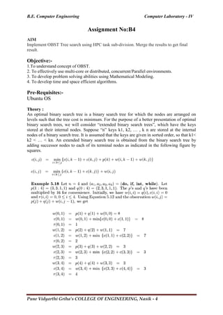
The major advantage of binary search trees over other data structures is that the
related sorting algorithms and search algorithms such as in-order traversal can be very
efficient; they are also easy to code. Binary search trees are a fundamental data
structure used to construct more abstract data structures such as sets, multisets, and
associative arrays.
Some of their disadvantages are as follows:The shape of the binary search tree totally
depends on the order of insertions and deletions, and it can become degenerated.
When inserting or searching for an element in a binary search tree, the key of each
visited node has to be compared with the key of the element to be inserted or found.
The keys in the binary search tree may be long and the run time may increase. After a
long intermixed sequence of random insertion and deletion, the expected height of the
tree approaches square root of the number of keys, √n, which grows much faster than
log n.
Types: There are many types of binary search trees:
1] AVL trees
2] Red-black trees
both forms of self-balancing binary search trees.
Operations:
Binary search trees support three main operations: insertion of elements, deletion of
elements, and lookup (checking whether a key is present).
1) Searching: Searching a binary search tree for a specific key can be a recursive or
an iterative process. We begin by examining the root node. If the tree is null, the
key we are searching for does not exist in the tree.
2) Insertion: Insertion begins as a search would begin; if the key is not equal to that
of the root, we search the left or right subtrees as before. Eventually, we will reach
an external node and add the new key-value pair (here encoded as a record
'newNode') as its right or left child, depending on the node's key..
3) Deletion: Simply remove the node from the tree. Deleting a node with one child:
remove the node and replace it with its child. Deleting a node with two children:
call the node to be deleted N. Do not delete N. Instead, choose either its in-order
successor node or its in-order predecessor node, R. Copy the value of R to N, then
recursively call delete on R until reaching one of the first two cases.
4) Tree traversal: Once the binary search tree has been created, its elements can be
retrieved in-order by recursively traversing the left subtree of the root node,
accessing the node itself, then recursively traversing the right subtree of the node,
continuing this pattern with each node in the tree as it's recursively accessed. As
with all binary trees, one may conduct a pre-order traversal or a post-order
traversal, but neither are likely to be useful for binary search trees. An in-order
traversal of a binary search tree will always result in a sorted list of node items
(numbers, strings or other comparable items).
Application:
1) Sort:
A binary search tree can be used to implement a simple sorting algorithm. Similar to
heap sort, we insert all the values we wish to sort into a new ordered data structure—
in this case a binary search tree—and then traverse it in order.
2) Priority queue operations
Conclusion:.
Hence, we have successfully implemented a function for Binary Search Tree using C
and Divide and Conquer Strategies.](https://image.slidesharecdn.com/finalcl-4manual2017-180104183918/85/COMPUTER-LABORATORY-4-LAB-MANUAL-BE-COMPUTER-ENGINEERING-5-320.jpg)
![B.E. Computer Engineering Computer Laboratory - IV
Pune Vidyarthi Griha’s COLLEGE OF ENGINEERING, Nasik - 4
Assignment No: A2
Title:
Using Divide and Conquer Strategies design a class for Concurrent Quick Sort using C++.
Aim:
Implement a Concurrent Quick Sort using divide and conquer strategy
Prerequsites :
Basic knowledge for concurrent c++ programming.
Ubuntu
Objectives:
1. Understand the importance Divide and Conquer Strategies
2. To learn Quick sort
Theory:
Quick Sort:
QuickSort is a Divide and Conquer algorithm. It picks an element as pivot and partitions the
given array around the picked pivot. There are many different versions of quickSort that pick
pivot in different ways.
1) Always pick first element as pivot.
2) Always pick last element as pivot
3) Pick a random element as pivot.
4) Pick median as pivot.
The key process in quickSort is partition(). Target of partitions is, given an array and an
element x of array as pivot, put x at its correct position in sorted array and put all smaller
elements (smaller than x) before x, and put all greater elements (greater than x) after x. All
this should be done in linear time.
Partition Algorithm:
There can be many ways to do partition. The logic is simple, we start from the leftmost
element and keep track of index of smaller (or equal to) elements as i. While traversing, if we
find a smaller element, we swap current element with pivot., Otherwise we ignore current
element.
partition(array, lower, upper)
{
pivot is array[lower]
while (true)
{ scan from right to left using index called RIGHT
STOP when locate an element that should be left of pivot
scan from left to right using index called LEFT
stop when locate an element that should be right of pivot
swap array[RIGHT] and array[LEFT]](https://image.slidesharecdn.com/finalcl-4manual2017-180104183918/85/COMPUTER-LABORATORY-4-LAB-MANUAL-BE-COMPUTER-ENGINEERING-6-320.jpg)
![B.E. Computer Engineering Computer Laboratory - IV
Pune Vidyarthi Griha’s COLLEGE OF ENGINEERING, Nasik - 4
if (RIGHT and LEFT cross)
pos = location where LEFT/RIGHT cross
swap pivot and array[pos]
all values left of pivot are <= pivot
all values right of pivot are >= pivot
return pos
end pos
} }
Example:
Time Complexity:
Best case complexity of quick sort is O(n log n)
Worst case Complexity is O (n2
)
Concurrent Quick sort:
Quicksort can be parallelized in a variety of ways. In the context of recursive decomposition,
during each call of QUICKSORT, the array is partitioned into two parts and each part is
solved recursively. Sorting the smaller arrays represents two completely independent sub
problems that can be solved in parallel. Therefore, one way to parallelize quicksort is to
execute it initially on a single process; then, when the algorithm performs its recursive calls
assign one of the sub problems to one process & other to another process. Now each of these
processes sorts its array by using quicksort. The algorithm terminates when the arrays cannot
be further partitioned. Upon termination, each process holds an element of the array, and the
sorted order can be recovered by traversing the processes.
Conclusion:
Thus we have studied and implemented concurrent Quick sort.](https://image.slidesharecdn.com/finalcl-4manual2017-180104183918/85/COMPUTER-LABORATORY-4-LAB-MANUAL-BE-COMPUTER-ENGINEERING-7-320.jpg)


![B.E. Computer Engineering Computer Laboratory - IV
Pune Vidyarthi Griha’s COLLEGE OF ENGINEERING, Nasik - 4
Assignment No: A5
Title:
To build a small compute cluster using Raspberry Pi/BBB modules to implement
Booths Multiplication Algorithm.
Aim:
Aim of this assignment is to build a small compute cluster using Raspberry Pi/BBB modules,
to perform Booths Multiplication Algorithm.
Prerequisites:
Beagle Bone Kit
Student should know basic concepts of Raspberry Pi/BBB.
Student should know basic concepts of Booths Multiplication Algorithm.
Objective:
1. To build a small compute cluster using Raspberry Pi/BBB modules, to perform
Booths Multiplication Algorithm.
Theory:
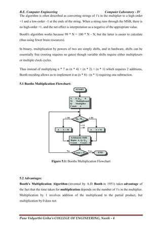
Booth's multiplication algorithm is a multiplication algorithm that multiplies two
signed binary numbers in two's complement notation. The algorithm was invented by
Andrew Donald Booth in 1950 while doing research on crystallography at Birkbeck College
in Bloomsbury, London.
Booth used desk calculators that were faster at shifting than adding and created the algorithm
to increase their speed. Booth's algorithm is of interest in the study of computer architecture.
Booth's algorithm examines adjacent pairs of bits of the N-bit multiplier Y in signed two's
complement representation, including an implicit bit below the least significant bit, y-1 = 0.
For each bit yi, for i running from 0 to N-1, the bits yi and yi-1are considered. Where these two
bits are equal, the product accumulator P is left unchanged. Where yi = 0 and yi-1 = 1, the
multiplicand times 2i
is added to P; and where yi = 1 and yi-1 = 0, the multiplicand times 2i
is
subtracted from P. The final value of P is the signed product.
The multiplicand and product are not specified; typically, these are both also in two's
complement representation, like the multiplier, but any number system that supports addition
and subtraction will work as well. As stated here, the order of the steps is not determined.
Typically, it proceeds from LSB to MSB, starting at i = 0; the multiplication by 2i
is then
typically replaced by incremental shifting of the P accumulator to the right between steps;
low bits can be shifted out, and subsequent additions and subtractions can then be done just
on the highest N bits of P.[1]
There are many variations and optimizations on these details.](https://image.slidesharecdn.com/finalcl-4manual2017-180104183918/85/COMPUTER-LABORATORY-4-LAB-MANUAL-BE-COMPUTER-ENGINEERING-18-320.jpg)

![B.E. Computer Engineering Computer Laboratory - IV
Pune Vidyarthi Griha’s COLLEGE OF ENGINEERING, Nasik - 4
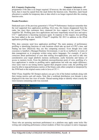
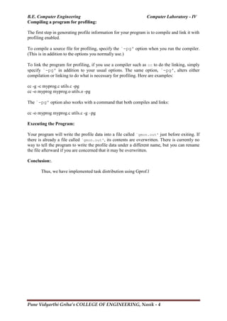
$ gcc –pg test.c –o test
$ ./test
$ gprof –b test gmon.out > output
$ more output
Output :
Each sample counts as 0.01 seconds.
% cumulative self self total
time seconds seconds calls s/call s/call name
71.90 30.17 30.17 1 30.17 30.17 C3
19.42 38.32 8.15 2 4.07 4.07 B2
7.99 41.67 3.35 1 3.35 3.35 C2
0.00 41.67 0.00 1 0.00 37.60 A
0.00 41.67 0.00 1 0.00 33.52 B1
0.00 41.67 0.00 1 0.00 0.00 C1
0.00 41.67 0.00 1 0.00 4.07 D
% time: the percent of self seconds from total program elapsed time.
cumulative seconds: the seconds cumulate from self seconds.
self seconds: total elapsed time called by its parents, not including its children‘s elapsed
time. equal to (self s/call)*(calls)
calls: total number for each subroutine called by its parents.
self s/call: elapsed time for each time called by its parents,not including its children‘s elapsed
time.
total s/call: total elapsed time called by its parents, including its children‘s elapsed time.
name: subroutine name.
Call Graph For Above Program:
Call graph
index %time self children called name
<spontaneous>
[1] 100.0 0.00 41.67 main[1]
0.00 37.60 1/1 A[2]
0.00 4.07 1/1 D[6]
------------------------------------------------------------------
0.00 37.60 1/1 main[1]
[2] 90.2 0.00 37.60 1 A[2]
0.00 33.52 1/1 B1[3]
4.07 0.00 1/2 B2[5]
------------------------------------------------------------------](https://image.slidesharecdn.com/finalcl-4manual2017-180104183918/85/COMPUTER-LABORATORY-4-LAB-MANUAL-BE-COMPUTER-ENGINEERING-40-320.jpg)
![B.E. Computer Engineering Computer Laboratory - IV
Pune Vidyarthi Griha’s COLLEGE OF ENGINEERING, Nasik - 4
0.00 33.52 1/1 A[2]
[3] 80.4 0.00 33.52 1 B1[3]
30.17 0.00 1/1 C3[4]
3.35 0.00 1/1 C2[7]
0.00 0.00 1/1 C1[8]
------------------------------------------------------------------
30.17 0.00 1/1 B1[3]
[4] 72.4 30.17 0.00 1 C3[4]
------------------------------------------------------------------
4.07 0.00 1/2 A[2]
4.07 0.00 1/2 D[6]
[5] 19.6 8.15 0.00 2 B2[5]
------------------------------------------------------------------
0.00 4.07 1/1 main[1]
[6] 9.8 0.00 4.07 1 D[6]
4.07 0.00 1/2 B2[5]
------------------------------------------------------------------
3.35 0.00 1/1 B1[3]
[7] 8.0 3.35 0.00 1 C2[7]
------------------------------------------------------------------
0.00 0.00 1/1 B1[3]
[8] 0.0 0.00 0.00 1 C1[8]
------------------------------------------------------------------
Several forms of output are available from the analysis.
1. The flat profile shows how much time your program spent in each function, and how
many times that function was called. If you simply want to know which functions
burn most of the cycles, it is stated concisely here.
2. The call graph shows, for each function, which functions called it, which other
functions it called, and how many times. There is also an estimate of how much time
was spent in the subroutines of each function. This can suggest places where you
might try to eliminate function calls that use a lot of time.
3. The annotated source listing is a copy of the program's source code, labeled with the
number of times each line of the program was executed.
Profiling has several steps:
You must compile and link your program with profiling enabled. See section
Compiling a Program for Profiling.
You must execute your program to generate a profile data file. See section Executing
the Program.
You must run gprof to analyze the profile data. See section gprof Command
Summary.
Gprof comes pre-installed with most of the Linux distributions, but if that‘s not the case
with your Linux distro, you can download and install it through a command line package
manager like apt-get or yum. For example, run the following command to download and
install gprof on Debian-based systems:
sudo apt-get install binutils](https://image.slidesharecdn.com/finalcl-4manual2017-180104183918/85/COMPUTER-LABORATORY-4-LAB-MANUAL-BE-COMPUTER-ENGINEERING-41-320.jpg)
![B.E. Computer Engineering Computer Laboratory - IV
Pune Vidyarthi Griha’s COLLEGE OF ENGINEERING, Nasik - 4
// ODD-Even Merge Sort
Program:
#include <stdio.h>
#include <stdlib.h>
#include <mpi.h>
int merge(double *ina, int lena, double *inb, int lenb, double *out) {
int i,j;
int outcount=0;
for (i=0,j=0; i<lena; i++) {
while ((inb[j] < ina[i]) && j < lenb) {
out[outcount++] = inb[j++];
}
out[outcount++] = ina[i];
}
while (j<lenb)
out[outcount++] = inb[j++];
return 0;
}
int domerge_sort(double *a, int start, int end, double *b) {
if ((end - start) <= 1) return 0;
int mid = (end+start)/2;
domerge_sort(a, start, mid, b);
domerge_sort(a, mid, end, b);
merge(&(a[start]), mid-start, &(a[mid]), end-mid, &(b[start]));
int i;
for (i=start; i<end; i++)
a[i] = b[i];
return 0;
}
int merge_sort(int n, double *a) {
double b[n];
domerge_sort(a, 0, n, b);
return 0;
}
void printstat(int rank, int iter, char *txt, double *la, int n) {
printf("[%d] %s iter %d: <", rank, txt, iter);
int i,j;
for (j=0; j<n-1; j++)
printf("%6.3lf,",la[j]);
printf("%6.3lf>n", la[n-1]);
}
void MPI_Pairwise_Exchange(int localn, double *locala, int sendrank, int recvrank,](https://image.slidesharecdn.com/finalcl-4manual2017-180104183918/85/COMPUTER-LABORATORY-4-LAB-MANUAL-BE-COMPUTER-ENGINEERING-47-320.jpg)
![B.E. Computer Engineering Computer Laboratory - IV
Pune Vidyarthi Griha’s COLLEGE OF ENGINEERING, Nasik - 4
MPI_Comm comm) {
/*
* the sending rank just sends the data and waits for the results;
* the receiving rank receives it, sorts the combined data, and returns
* the correct half of the data.
*/
int rank;
double remote[localn];
double all[2*localn];
const int mergetag = 1;
const int sortedtag = 2;
MPI_Comm_rank(comm, &rank);
if (rank == sendrank) {
MPI_Send(locala, localn, MPI_DOUBLE, recvrank, mergetag,
MPI_COMM_WORLD);
MPI_Recv(locala, localn, MPI_DOUBLE, recvrank, sortedtag, MPI_COMM_WORLD,
MPI_STATUS_IGNORE);
} else {
MPI_Recv(remote, localn, MPI_DOUBLE, sendrank, mergetag,
MPI_COMM_WORLD, MPI_STATUS_IGNORE);
merge(locala, localn, remote, localn, all);
int theirstart = 0, mystart = localn;
if (sendrank > rank) {
theirstart = localn;
mystart = 0;
}
MPI_Send(&(all[theirstart]), localn, MPI_DOUBLE, sendrank, sortedtag,
MPI_COMM_WORLD);
int i;
for (i=mystart; i<mystart+localn; i++)
locala[i-mystart] = all[i];
}
}
int MPI_OddEven_Sort(int n, double *a, int root, MPI_Comm comm)
{
int rank, size, i;
double *local_a;
// get rank and size of comm
MPI_Comm_rank(comm, &rank); //&rank = address of rank
MPI_Comm_size(comm, &size);
local_a = (double *) calloc(n / size, sizeof(double));
// scatter the array a to local_a
MPI_Scatter(a, n / size, MPI_DOUBLE, local_a, n / size, MPI_DOUBLE,
root, comm);](https://image.slidesharecdn.com/finalcl-4manual2017-180104183918/85/COMPUTER-LABORATORY-4-LAB-MANUAL-BE-COMPUTER-ENGINEERING-48-320.jpg)
![B.E. Computer Engineering Computer Laboratory - IV
Pune Vidyarthi Griha’s COLLEGE OF ENGINEERING, Nasik - 4
// sort local_a
merge_sort(n / size, local_a);
//odd-even part
for (i = 1; i <= size; i++) {
printstat(rank, i, "before", local_a, n/size);
if ((i + rank) % 2 == 0) { // means i and rank have same nature
if (rank < size - 1) {
MPI_Pairwise_Exchange(n / size, local_a, rank, rank + 1, comm);
}
} else if (rank > 0) {
MPI_Pairwise_Exchange(n / size, local_a, rank - 1, rank, comm);
}
}
printstat(rank, i-1, "after", local_a, n/size);
// gather local_a to a
MPI_Gather(local_a, n / size, MPI_DOUBLE, a, n / size, MPI_DOUBLE,
root, comm);
if (rank == root)
printstat(rank, i, " all done ", a, n);
return MPI_SUCCESS;
}
int main(int argc, char **argv) {
MPI_Init(&argc, &argv);
int n = argc-1;
double a[n];
int i;
for (i=0; i<n; i++)
a[i] = atof(argv[i+1]);
MPI_OddEven_Sort(n, a, 0, MPI_COMM_WORLD);
MPI_Finalize();
return 0;
}](https://image.slidesharecdn.com/finalcl-4manual2017-180104183918/85/COMPUTER-LABORATORY-4-LAB-MANUAL-BE-COMPUTER-ENGINEERING-49-320.jpg)
![B.E. Computer Engineering Computer Laboratory - IV
Pune Vidyarthi Griha’s COLLEGE OF ENGINEERING, Nasik - 4
Assignment No: C1
Aim:
Write HTML5 programming techniques to compile a text PDF file integrating Latex
Objective:
To learn the programming techniques in HTML5
Theory:
Introduction:
The Web Hypertext Application Technology Working Group (WHATWG) began work on
the new standard in 2004. At that time, HTML 4.01 had not been updated since 2000, and
the World Wide Web Consortium (W3C) was focusing future developments on XHTML 2.0.
In 2009, the W3C allowed the XHTML 2.0 Working Group's charter to expire and decided
not to renew it. W3C and WHATWG are currently working together on the development of
HTML5.
While some features of HTML5 are often compared to Adobe Flash, the two technologies are
very different. Both include features for playing audio and video within web pages, and for
using Scalable Vector Graphics. However, HTML5 on its own cannot be used for animation
or interactivity – it must be supplemented with CSS3 or JavaScript. There are many Flash
capabilities that have no direct counterpart in HTML5. See Comparison of HTML5 and
Flash.
Although HTML5 has been well known among web developers for years, its interactive
capabilities became a topic of mainstream media around April 2010[11][12][13][14]
after Apple
Inc's then-CEO Steve Jobs issued a public letter titled "Thoughts on Flash" where he
concluded that "Flash is no longer necessary to watch video or consume any kind of web
content" and that "new open standards created in the mobile era, such as HTML5, will
win".[15]
This sparked a debate in web development circles suggesting that, while HTML5
provides enhanced functionality, developers must consider the varying browser support of the
different parts of the standard as well as other functionality differences between HTML5 and
Flash.[16]
In early November 2011, Adobe announced that it would discontinue development
of Flash for mobile devices and reorient its efforts in developing tools using HTML5
Features and APIs:
The W3C proposed a greater reliance on modularity as a key part of the plan to make
faster progress, meaning identifying specific features, either proposed or already existing in
the spec, and advancing them as separate specifications. Some technologies that were
originally defined in HTML5 itself are now defined in separate specifications:
HTML Working Group – HTML Canvas 2D Context
Web Apps WG – Web Messaging, Web Workers, Web Storage, WebSocket API,
Server-Sent Events
IETF HyBi WG – WebSocket Protocol
WebRTC WG – WebRTC
W3C Web Media Text Tracks CG – WebVTT
After the standardization of the HTML5 specification in October 2014, the core vocabulary
and features are being extended in four ways. Likewise, some features that were removed](https://image.slidesharecdn.com/finalcl-4manual2017-180104183918/85/COMPUTER-LABORATORY-4-LAB-MANUAL-BE-COMPUTER-ENGINEERING-50-320.jpg)
![B.E. Computer Engineering Computer Laboratory - IV
Pune Vidyarthi Griha’s COLLEGE OF ENGINEERING, Nasik - 4
begin{document}
Hello world!
end{document}
Spaces
The LaTeX compiler normalises whitespace so that whitespace characters, such as [space] or
[tab], are treated uniformly as "space": several consecutive "spaces" are treated as one,
"space" opening a line is generally ignored, and a single line break also yields ―space‖. A
double line break (an empty line), however, defines the end of a paragraph; multiple empty
lines are also treated as the end of a paragraph. An example of applying these rules is
presented below: the left-hand side shows the user's input (.tex), while the right-hand side
depicts the rendered output (.dvi/.pdf/.ps).
It does not matter whether
you
enter one or several
spaces
after a word.
An empty line starts a
new
paragraph.
It does not matter whether you enter one or several
spaces after a word.
An empty line starts a new paragraph.
Reserved Characters
The following symbols are reserved characters that either have a special meaning under
LaTeX or are unavailable in all the fonts. If you enter them directly in your text, they will
normally not print but rather make LaTeX do things you did not intend.
# $ % ^ & _ { } ~
As you will see, these characters can be used in your documents all the same by adding a
prefix backslash:
# $ % ^{} & _ { } ~{} textbackslash{}
The backslash character cannot be entered by adding another backslash in front of it ();
this sequence is used for line breaking. For introducing a backslash in math mode, you can
use backslash instead.
The commands ~ and ^ produce respectively a tilde and a hat which is placed over the next
letter. For example ~n gives ñ. That's why you need braces to specify there is no letter as
argument. You can also use textasciitilde and textasciicircum to enter these characters; or
other commands .
If you want to insert text that might contain several particular symbols (such as URIs), you
can consider using the verb command, which will be discussed later in the section on
formatting. For source code, see Source Code Listings](https://image.slidesharecdn.com/finalcl-4manual2017-180104183918/85/COMPUTER-LABORATORY-4-LAB-MANUAL-BE-COMPUTER-ENGINEERING-52-320.jpg)

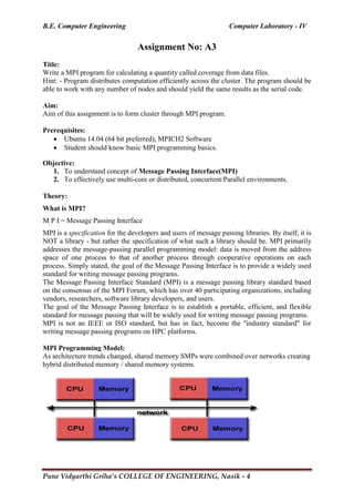
1) The document describes writing an MPI program to calculate a quantity called coverage from data files in a distributed manner across a cluster. 2) MPI (Message Passing Interface) is a standard for writing programs that can run in parallel on multiple processors. The program should distribute the computation efficiently across the cluster nodes and yield the same results as a serial code. 3) The MPI program structure involves initialization, processes running concurrently on nodes, communication between processes, and finalization. Communicators define which processes can communicate.