Correlation and Regression for agriculture.pdf

1. Correlation and regression
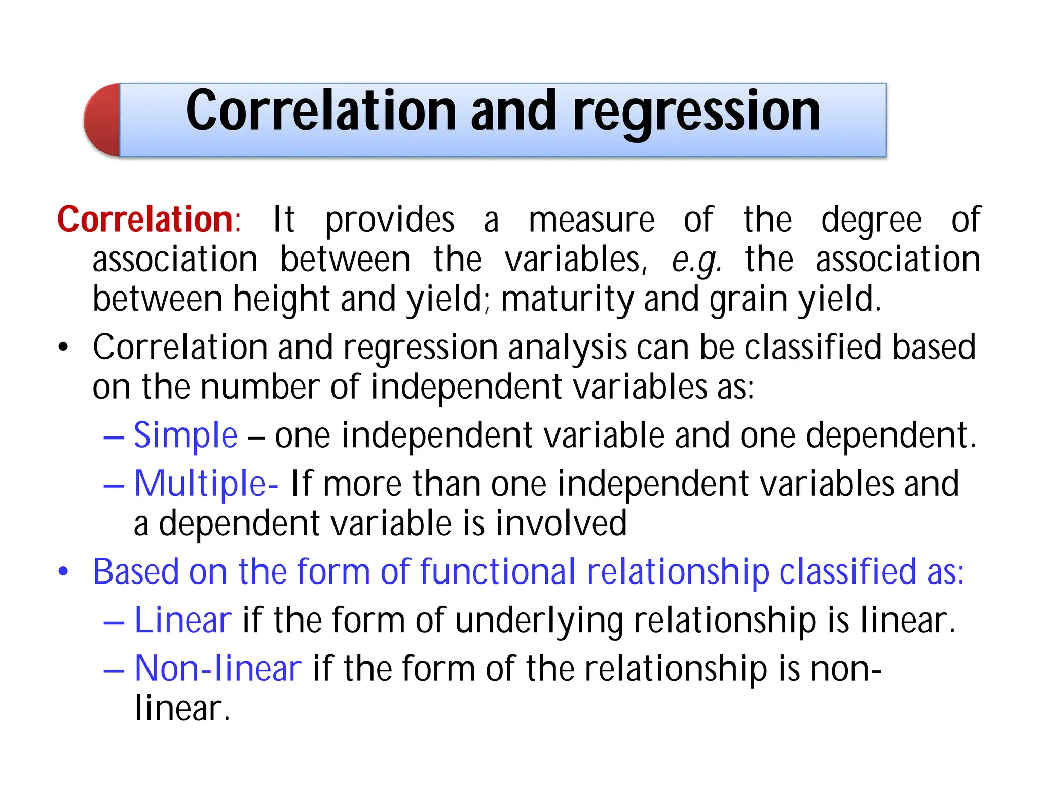
Correlation: It provides a measure of the degree of
association between the variables, e.g. the association
between height and yield; maturity and grain yield.
• Correlation and regression analysis can be classified based
on the number of independent variables as:
– Simple – one independent variable and one dependent.
– Multiple- If more than one independent variables and
a dependent variable is involved
• Based on the form of functional relationship classified as:
– Linear if the form of underlying relationship is linear.
– Non-linear if the form of the relationship is non-
linear.

2. • Common regression and correlation analysis can
be classified into:
• Simple linear regression and correlation analysis.
• Multiple linear regression and correlation analysis.
The most commonly used correlation is linear correlation,
correlation coefficient (‘r’.)
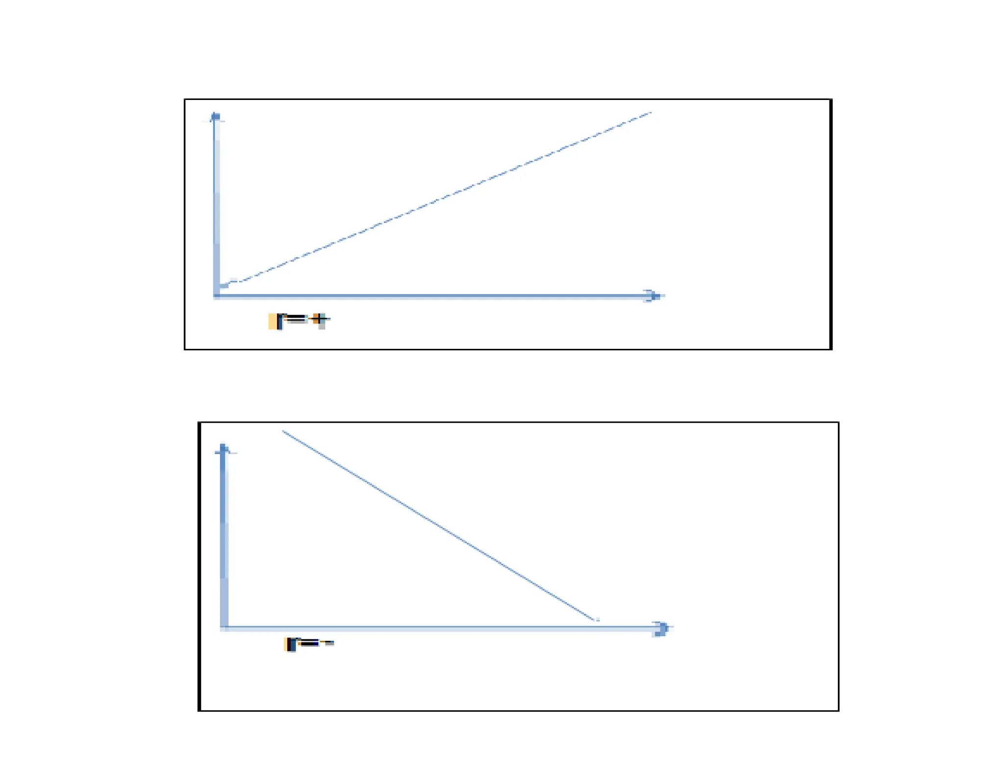
The value of r is within the range of -1 to +1.
R=o shows no-linear relationship

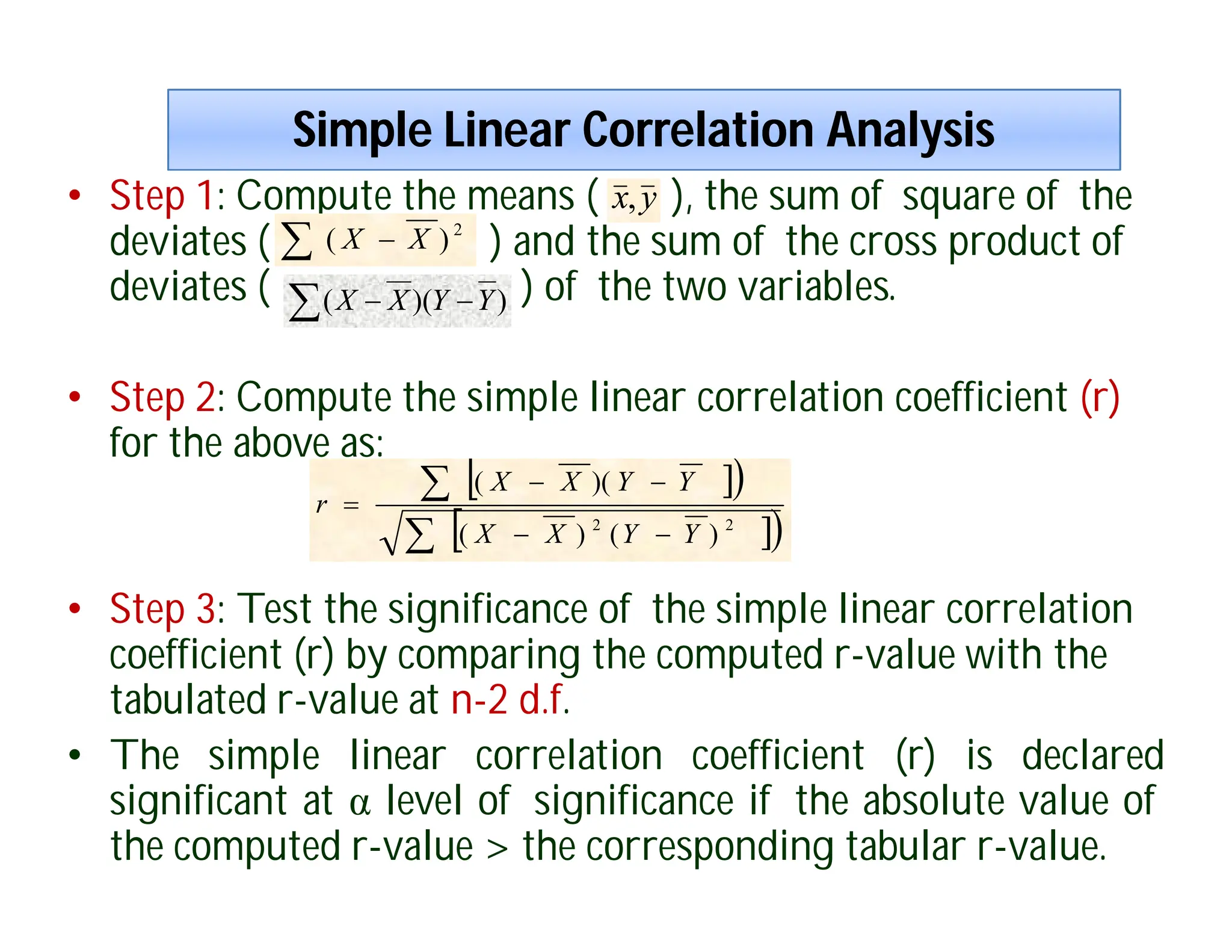
4. Simple Linear Correlation Analysis
Simple Linear Correlation Analysis
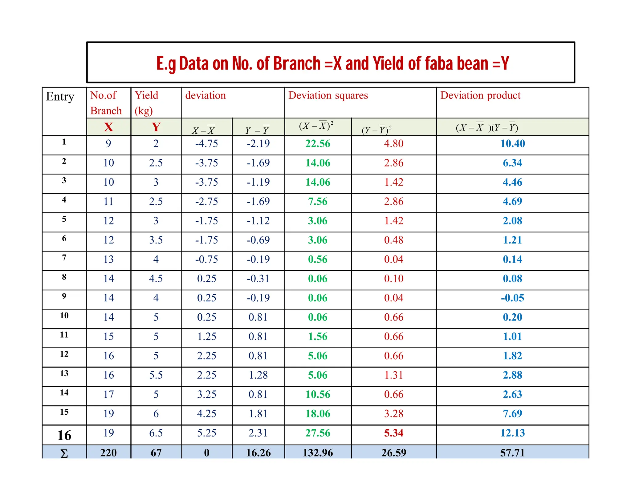
• Step 1: Compute the means ( ), the sum of square of the
deviates ( ) and the sum of the cross product of
deviates ( ) of the two variables.
• Step 2: Compute the simple linear correlation coefficient (r)
for the above as:
• Step 3: Test the significance of the simple linear correlation
coefficient (r) by comparing the computed r-value with the
tabulated r-value at n-2 d.f.
• The simple linear correlation coefficient (r) is declared
significant at α level of significance if the absolute value of
the computed r-value > the corresponding tabular r-value.
y
x,
  2
)
( X
X
 
 )
)(
( Y
Y
X
X

 

 







2
2
)
(
)
(
)(
(
Y
Y
X
X
Y
Y
X
X
r

5. E.g Data on No. of Branch =X and Yield of faba bean =Y
Entry No.of
Branch
Yield
(kg)
deviation Deviation squares Deviation product
X Y
1 9 2 -4.75 -2.19 22.56 4.80 10.40
2 10 2.5 -3.75 -1.69 14.06 2.86 6.34
3 10 3 -3.75 -1.19 14.06 1.42 4.46
4 11 2.5 -2.75 -1.69 7.56 2.86 4.69
5 12 3 -1.75 -1.12 3.06 1.42 2.08
6 12 3.5 -1.75 -0.69 3.06 0.48 1.21
7 13 4 -0.75 -0.19 0.56 0.04 0.14
8 14 4.5 0.25 -0.31 0.06 0.10 0.08
9 14 4 0.25 -0.19 0.06 0.04 -0.05
10 14 5 0.25 0.81 0.06 0.66 0.20
11 15 5 1.25 0.81 1.56 0.66 1.01
12 16 5 2.25 0.81 5.06 0.66 1.82
13 16 5.5 2.25 1.28 5.06 1.31 2.88
14 17 5 3.25 0.81 10.56 0.66 2.63
15 19 6 4.25 1.81 18.06 3.28 7.69
16 19 6.5 5.25 2.31 27.56 5.34 12.13
 220 67 0 16.26 132.96 26.59 57.71
X
X  Y
Y 
2
)
( X
X  2
)
( Y
Y  )
)(
( Y
Y
X
X 


6. Data on Biomass yield (BM) and Grain yield of barley (Y)
No.
No. Gen.
Gen. BM (X)
BM (X) GY(Y)
GY(Y)
Deviation
Deviation Deviation
Deviation squares
squares
D
Deviation
eviation product
product
1 P1 43.1 20.6 -5.88 -0.65 34.57 0.42 3.82
2 P2 63.0 24.7 14.02 3.45 196.56 11.90 48.37
3 F1 54.2 26.1 5.22 4.88 27.25 23.77 25.47
4 F2 42.6 18.9 -6.38 -2.27 40.70 5.14 14.48
5 B1 44.6 20.0 -4.38 -1.23 19.18 1.51 5.39
6 B2 50.4 22.3 1.42 1.11 2.02 1.24 1.58
7 P1 54.7 27.7 5.72 6.50 32.72 42.25 37.18
8 P2 39.5 11.9 -9.48 -9.30 89.87 86.49 88.16
9 F1 47.8 22.7 -1.18 1.48 1.39 2.18 -1.75
10 F2 36.7 15.5 -12.28 -5.67 150.80 32.11 69.63
11 B1 57.3 25.1 8.32 3.89 69.22 15.11 32.36
12 B2 48.8 21.6 -0.18 0.41 0.03 0.17 -0.07
13 P1 52.0 24.7 3.02 3.50 9.12 12.25 10.57
14 P2 61.1 26.0 12.12 4.83 146.89 23.28 58.54
15 F1 49.0 24.0 0.02 2.78 0.00 7.70 0.06
16 F2 46.8 20.7 -2.18 -0.50 4.75 0.25 1.09
17 B1 39.7 19.5 -9.28 -1.69 86.12 2.84 15.68
18 B2 50.4 21.9 1.42 0.72 2.02 0.52 1.02
 881.6
881.6 393.8
393.8 0.06
0.06 12.2
12.2 913.23 269.1
269.1 411.59
mean 48.98 21.88
2
)
( X
X  2
)
( Y
Y 
X
X  Y
Y 

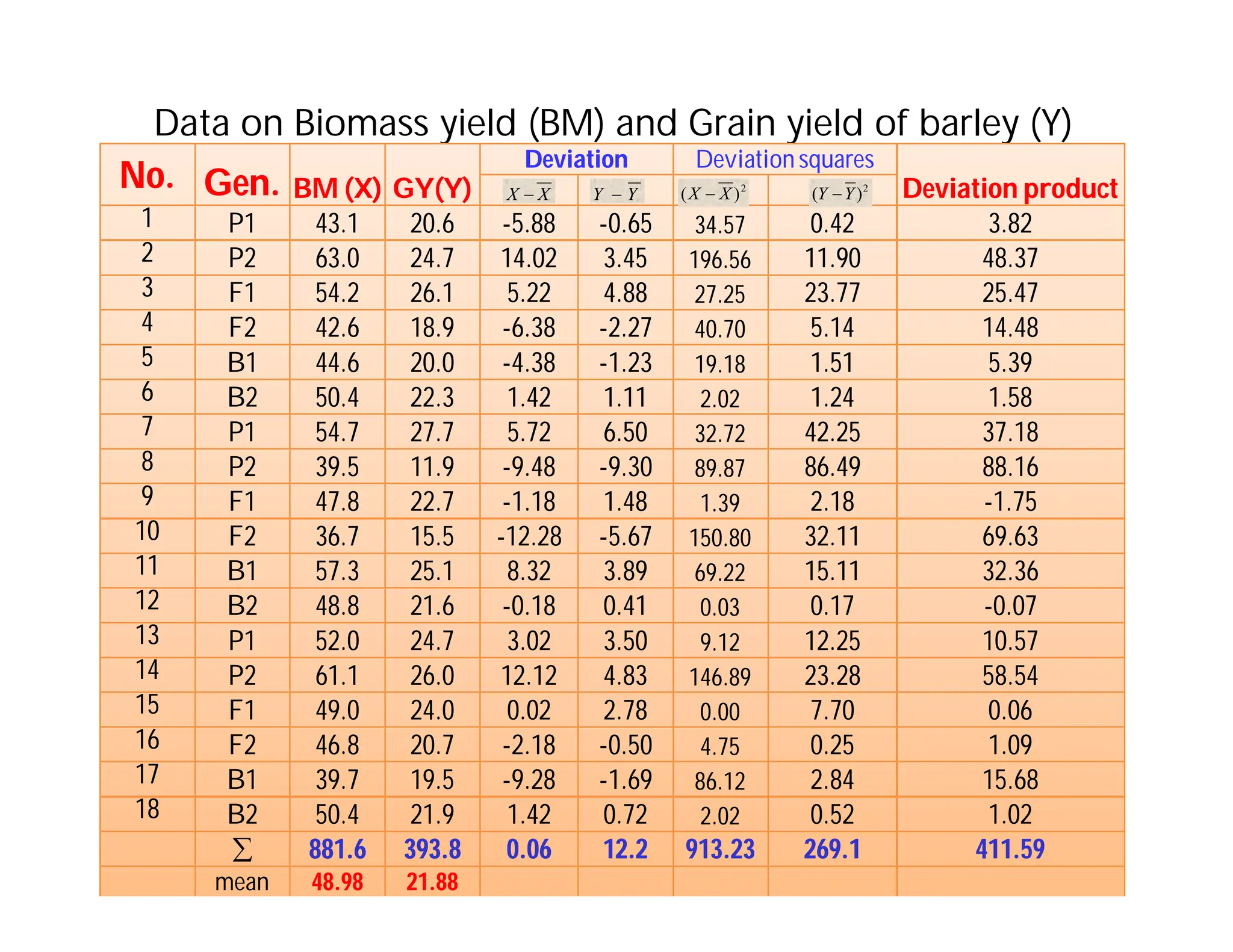
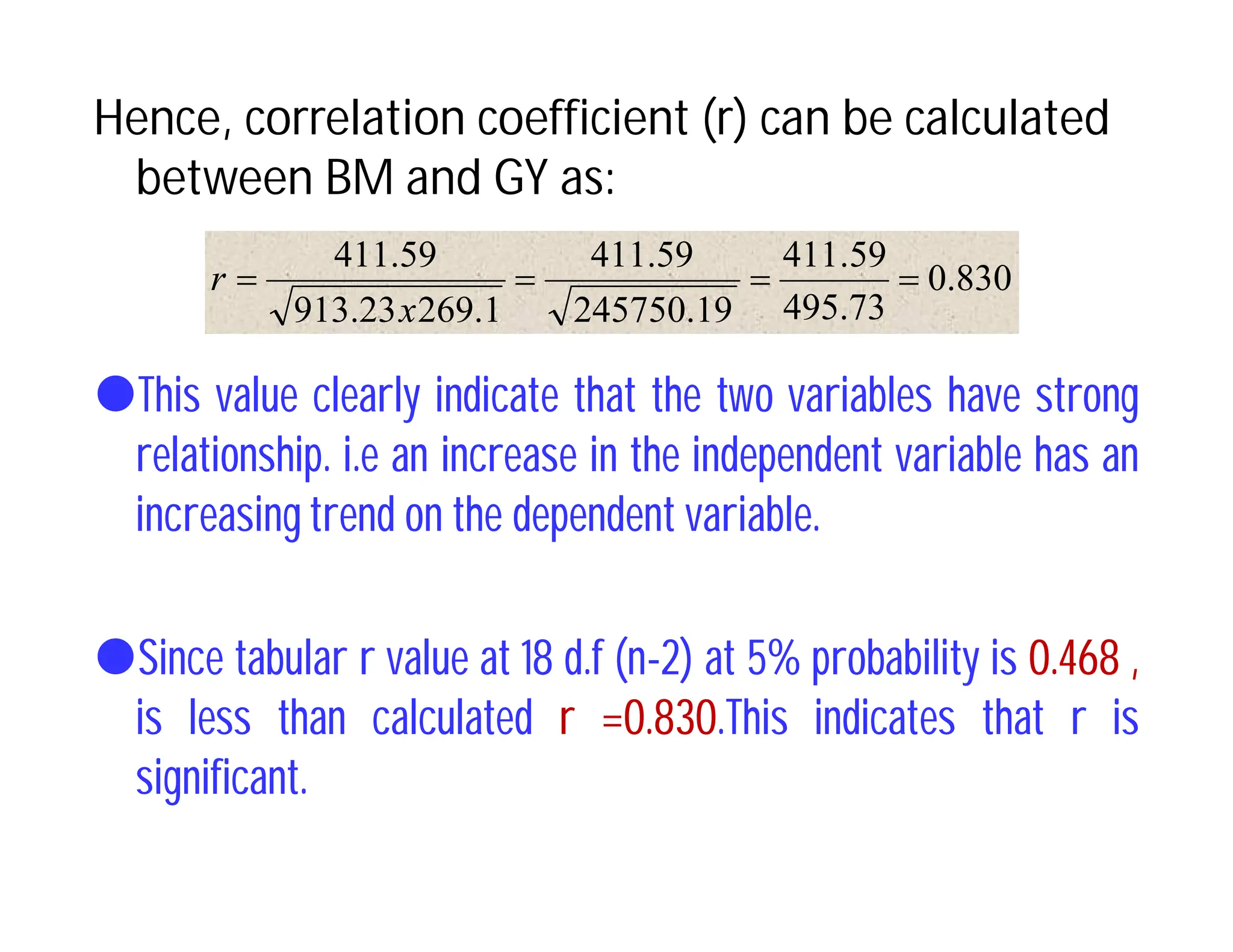
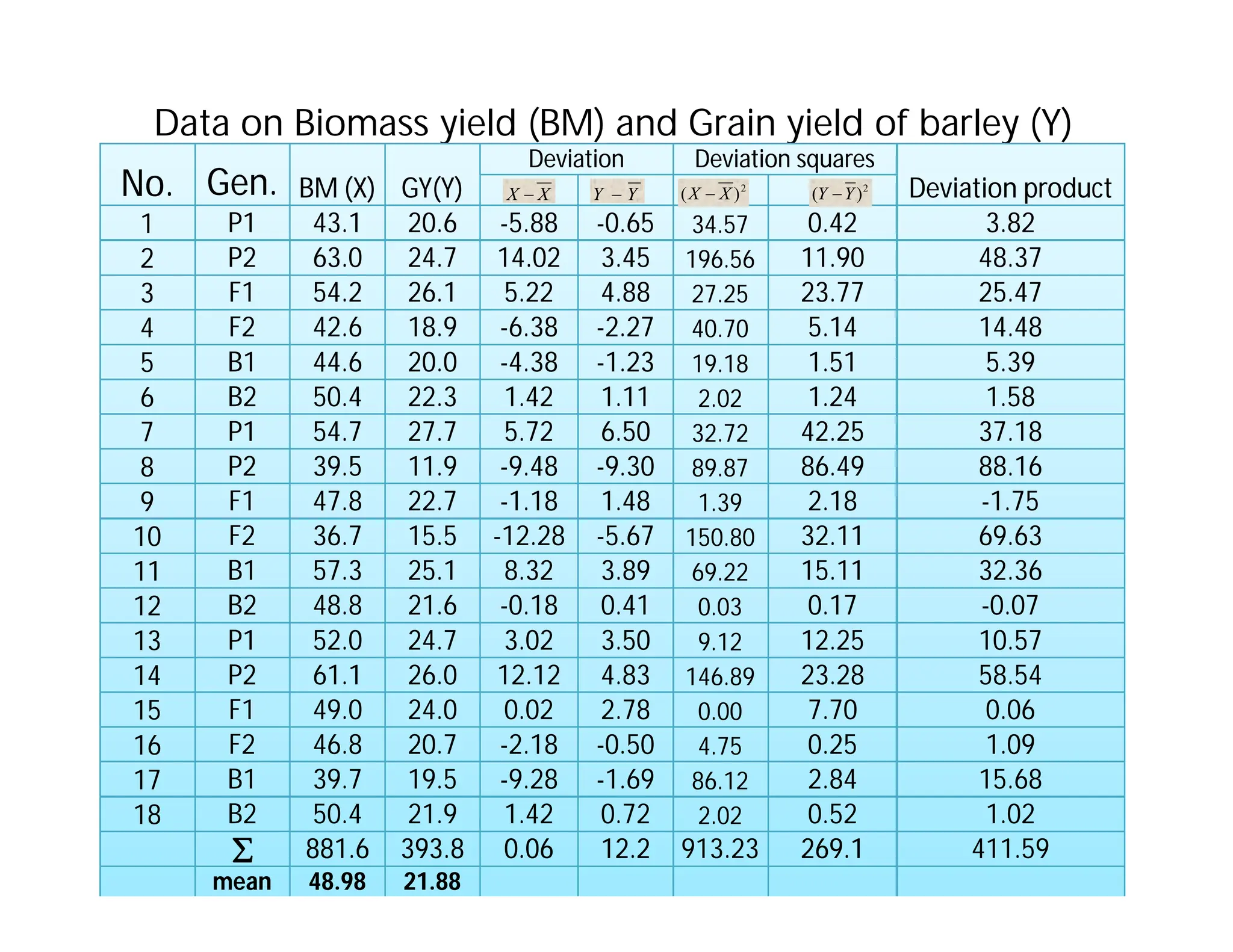
7. Hence, correlation coefficient (r) can be calculated
between BM and GY as:
This value clearly indicate that the two variables have strong
relationship. i.e an increase in the independent variable has an
increasing trend on the dependent variable.
Since tabular r value at 18 d.f (n-2) at 5% probability is 0.468 ,
is less than calculated r =0.830.This indicates that r is
significant.
0.830
495.73
59
.
411
245750.19
411.59
269.1
913.23
411.59




x
r

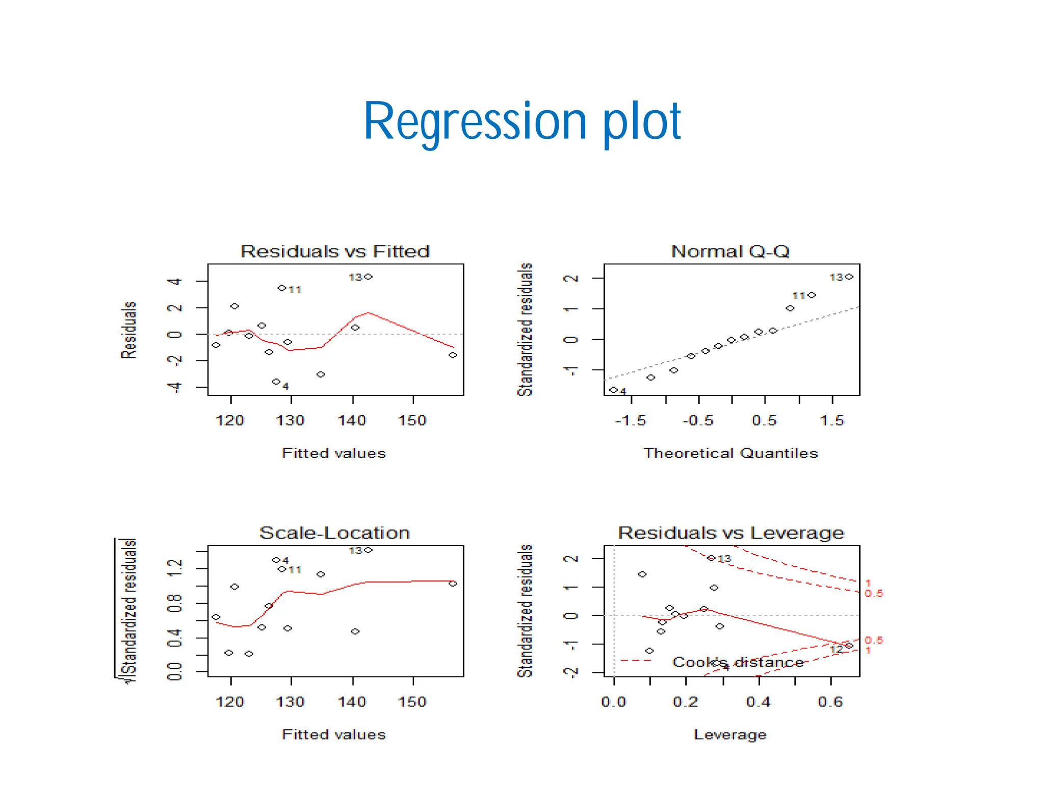
8. Regression
 It describes the effect of one or more variables (designated as
independent variables) on a single variable (designated as
the dependent variable).
 It expresses the dependent variable as a function of
independent variable(s).
 Regression is a mathematical means of expression of the
intensity of relationship between two variables.
 It shows the quantitative change of dependent variable
whenever there is certain unit of change on the independent
variable.
 For regression analysis, it is important to clearly distinguish
between the dependent and independent variables.

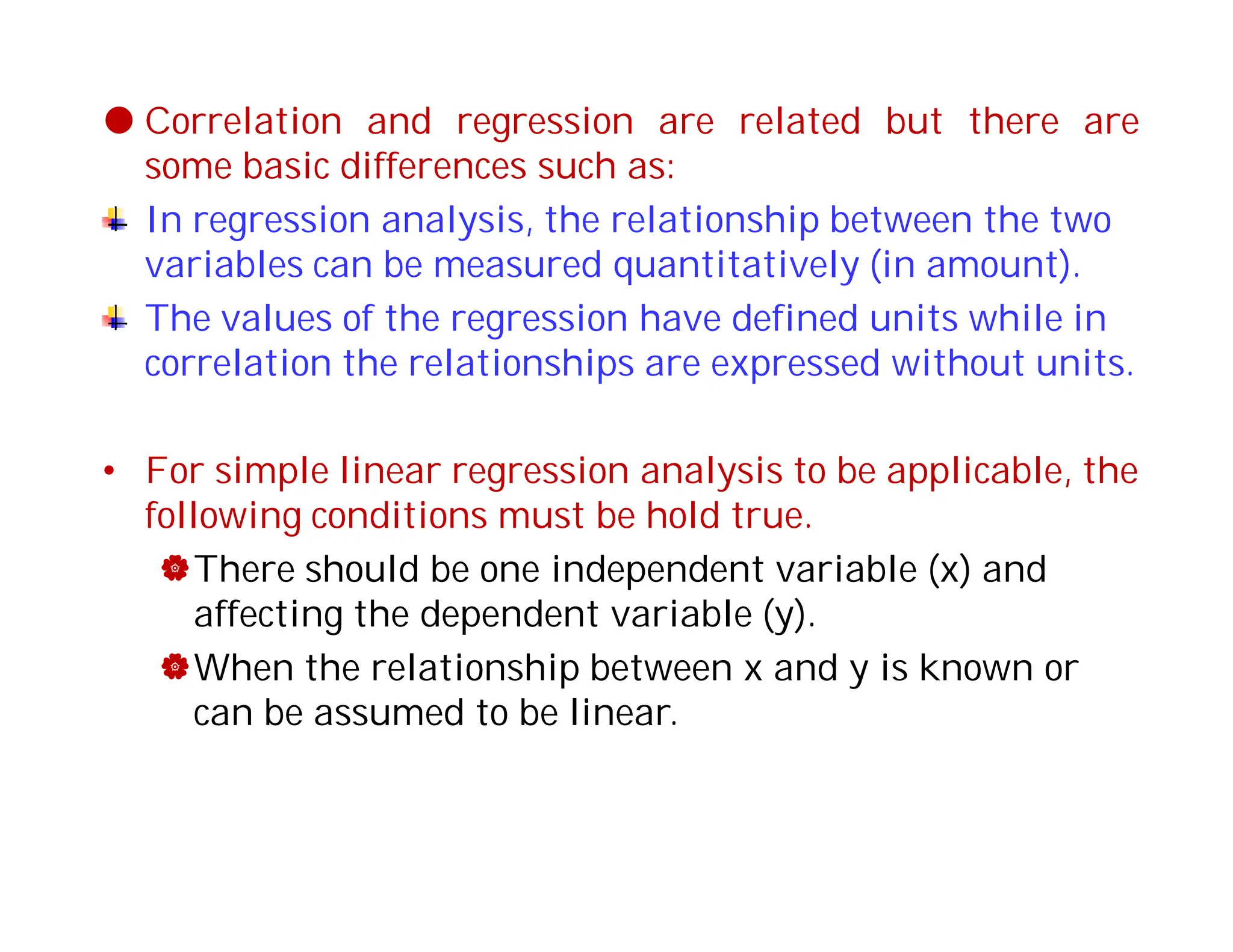
9.  Correlation and regression are related but there are
some basic differences such as:
In regression analysis, the relationship between the two
variables can be measured quantitatively (in amount).
The values of the regression have defined units while in
correlation the relationships are expressed without units.
• For simple linear regression analysis to be applicable, the
following conditions must be hold true.
There should be one independent variable (x) and
affecting the dependent variable (y).
When the relationship between x and y is known or
can be assumed to be linear.

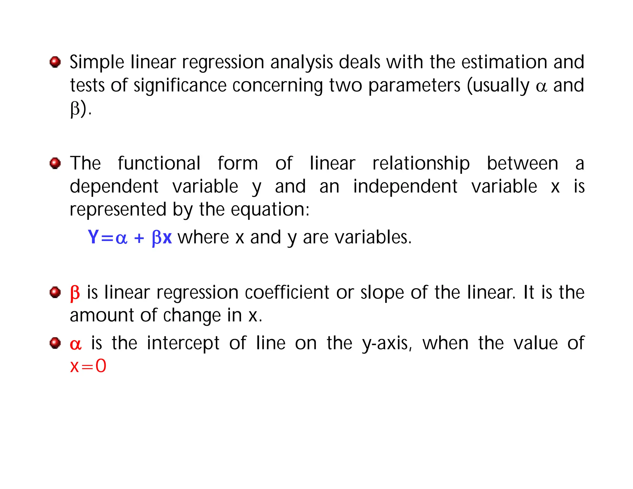
10. Simple linear regression analysis deals with the estimation and
tests of significance concerning two parameters (usually  and
).
The functional form of linear relationship between a
dependent variable y and an independent variable x is
represented by the equation:
Y= + x where x and y are variables.
 is linear regression coefficient or slope of the linear. It is the
amount of change in x.
 is the intercept of line on the y-axis, when the value of
x=0

11. Data on Biomass yield (BM) and Grain yield of barley (Y)
No.
No. Gen.
Gen. BM (X)
BM (X) GY(Y)
GY(Y)
Deviation
Deviation Deviation
Deviation squares
squares
D
Deviation
eviation product
product
1 P1 43.1 20.6 -5.88 -0.65 34.57 0.42 3.82
2 P2 63.0 24.7 14.02 3.45 196.56 11.90 48.37
3 F1 54.2 26.1 5.22 4.88 27.25 23.77 25.47
4 F2 42.6 18.9 -6.38 -2.27 40.70 5.14 14.48
5 B1 44.6 20.0 -4.38 -1.23 19.18 1.51 5.39
6 B2 50.4 22.3 1.42 1.11 2.02 1.24 1.58
7 P1 54.7 27.7 5.72 6.50 32.72 42.25 37.18
8 P2 39.5 11.9 -9.48 -9.30 89.87 86.49 88.16
9 F1 47.8 22.7 -1.18 1.48 1.39 2.18 -1.75
10 F2 36.7 15.5 -12.28 -5.67 150.80 32.11 69.63
11 B1 57.3 25.1 8.32 3.89 69.22 15.11 32.36
12 B2 48.8 21.6 -0.18 0.41 0.03 0.17 -0.07
13 P1 52.0 24.7 3.02 3.50 9.12 12.25 10.57
14 P2 61.1 26.0 12.12 4.83 146.89 23.28 58.54
15 F1 49.0 24.0 0.02 2.78 0.00 7.70 0.06
16 F2 46.8 20.7 -2.18 -0.50 4.75 0.25 1.09
17 B1 39.7 19.5 -9.28 -1.69 86.12 2.84 15.68
18 B2 50.4 21.9 1.42 0.72 2.02 0.52 1.02
881.6
881.6 393.8
393.8 0.06
0.06 12.2
12.2 913.23 269.1
269.1 411.59
mean 48.98 21.88
2
)
( X
X  2
)
( Y
Y 
X
X  Y
Y 

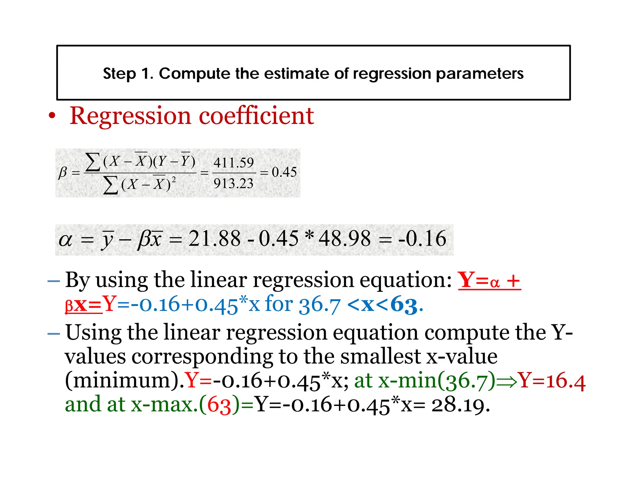
12. Step 1. Compute the estimate of regression parameters
• Regression coefficient
– By using the linear regression equation: Y= +
x=Y=-0.16+0.45*x for 36.7 <x<63.
– Using the linear regression equation compute the Y-
values corresponding to the smallest x-value
(minimum).Y=-0.16+0.45*x; at x-min(36.7)Y=16.4
and at x-max.(63)=Y=-0.16+0.45*x= 28.19.
0.45
913.23
411.59
)
(
)
)(
(
2








X
X
Y
Y
X
X

-0.16
48.98
*
0.45
-
21.88 


 x
y 


13. Regression plot