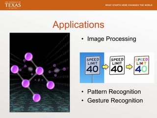
Connected Components Labeling
  Term Project: CS395T, Software for Multicore Processors


                  Hemanth Kumar Mantri
                  Siddharth Subramanian
                      Kumar Ashish
Big Picture
• Studied, Implemented and Evaluated
  various parallel algorithms for Connected
  Components Labeling in Graphs
• Two Architectures
  – CPU (OpenMP) and GPU (CUDA)
• Different types of graphs
• Propose simple Autotuned approach for
  choosing best technique for a graph
Our Menu
•   Motivation
•   Definitions
•   Basic Algorithms
•   Optimizations
•   Datasets and Experiments
•   Autotuning
•   Future Scope
Our Menu
•   Motivation
•   Definitions
•   Basic Algorithms
•   Optimizations
•   Datasets and Experiments
•   Autotuning
•   Future Scope
Why Connected Components?
• Identify vertices that
  form a connected set in
  a Graph
• Used in:
   – Pattern Recognition
   – Physics
      • Identify Clusters
   – Biology
      • DNA components
   – Social Network Analysis
Applications
• Physics               • Image Processing
  – Identify Clusters
• Biology
  – Components in DNA


                        • Pattern Recognition
                        • Gesture Recognition
Sequential Implementation
• Disjoint Set Union
  –   MakeSet
  –   Union
  –   Link
  –   FindSet


• Depth First Search
Our Menu
•   Motivation
•   Definitions
•   Basic Algorithms
•   Optimizations
•   Datasets and Experiments
•   Autotuning
•   Future Scope
Rooted Star
• Directed tree of h = 1

• Root points to itself

• All children point to the
  root

• Root is called the
  representative of a
  connected component
Hooking
• (i, j) is an edge in the
  graph
• If i and j are currently
  in different trees
• Merge the two trees
  in to one
• Make representative
  of one, point to the
  representative of the
  other
Breaking Ties
• Merging two trees T1 and T2,
• Whose representative should be
  changed?
  – Toss a coin and choose a winner
  – Tree with lower(higher) index wins always
  – Alternate between iterations (Even, Odd)
  – Tree with greater height wins
Pointer Jumping
• Move a node higher
  in the tree

• Single Level

• Multi Level

• Final Aim
  – Form Rooter Stars
EXAMPLE
Start From Singletons
Hooking
Pointer Jumping
Our Menu
•   Motivation
•   Definitions
•   Basic Algorithms
•   Optimizations
•   Datasets and Experiments
•   Autotuning
•   Future Scope
SV Algorithm
Revised Deterministic Algorithm
Our Menu
•   Motivation
•   Definitions
•   Basic Algorithms
•   Optimizations
•   Datasets and Experiments
•   Autotuning
•   Future Scope
CPU Optimizations
• Single Instance edge storage
  – (u, v) is same as (v, u)
  – Reduced Memory Footprint
     • Support large graphs
  – Smaller traversal overhead
     • Every iteration needs to see all edges
• Unconditional Hooking
  – Calling at appropriate iteration helps in
    decreasing the number of iterations
Multi Level Pointer Jumping
• Only form stars in
  every iteration
• No overhead in
  determining if a node
  is part of a star
OpenMP Scheduling
• Static

• Dynamic

• Guided Scheduling
  – Gave best performance
Hide Inactive Edges
• If two ends of an edge
  are part of same
  connected
  component, hide
  them
• Save time for next
  iterations
For GPU
• Different from PRAM Model
   – Threads are grouped into Thread Blocks
   – Requires explicit synchronization across TBs

• 64 bit for representing an edge
   – Reduced Random Reads
   – Read edge in single memory transaction

• In first Iteration hook neighbors instead of their parents
   – Reduced irregular reads

• GeForce GTX 480
   – Use 1024 threads per block
Our Menu
•   Motivation
•   Definitions
•   Basic Algorithms
•   Optimizations
•   Datasets and Experiments
•   Autotuning
•   Future Scope
Datasets
• Random Graphs
  – 1M to 7M nodes, average degree 5
• RMAT Graphs
  – Synthetic Social Networks
  – 1M to 7M nodes
• Real World Data (From SNAP, by Leskovec)
  – Road Networks:
     • California
     • Pennsylvania
     • Texas
  – Web Graphs
     • Google Web
     • Berkeley-Stanford domains
Execution Environment
• CPU (Faraday): A 48 core Intel Xeon
  E7540 (2.00 GHz), with 18 MB cache, 132
  GB RAM
• GPU (Gleim): GeForce GTX 480 with 1.5
  GB shared memory and 177.4 GB/s
  memory bandwidth. It was attached to a
  Quadcore Intel Xeon CPU (2.40 GHz)
  running CUDA Toolkit/SDK version 4.1.
  The host machine had 6 GB RAM.
Random Graphs CPU – Scaling with threads
RMAT-Graphs CPU – Scaling with threads
Web graphs CPU – Scaling with threads
Road network CPU – Scaling with threads
Random graph – Scaling with vertices
R-MAT – Scaling with vertices
GPU on Random and RMAT
Real World Graphs
Our Menu
•   Motivation
•   Definitions
•   Basic Algorithms
•   Optimizations
•   Datasets and Experiments
•   Analysis and Autotuning
•   Future Scope
What is Autotuning?
• Automatic process for selecting one out of several
  possible solutions to a computational problem.
• The solutions may differ in the
   – algorithm (quicksort vs selection sort)
   – implementation (loop unroll).
• The versions may result from
   – transformations (unroll, tile, interchange)
• The versions could be generated by
   – programmer manually (coding or directives)
   – compiler automatically
How?
• Have various ways to do hooking, pointer
  jumping
• Characterize graphs based on some
  features
• Employ the best technique for a given
  graph
Performance Deciders
• Number of Iterations
  – Each iteration needs to traverse the whole set
    of edges
• Pointer Jumps
  – Higher the root node, more the work
• Trade off
  – More iterations and Single level jump in each
    iteration
  – Less iterations with Multi Level jumps
Choosing Right Approach
• More iterations and Single level jump in each
  iteration
  – Good for graphs with less edges and less
    diameter
  – If edges is constant, works well for social
    networks
• Less iterations with Multi Level jumps
  – Good for graphs with large diameter
  – Very good scalability – Good for GPU
  – Road Network
Graph Types
• Road Networks
  – Large diameter
  – Forms very deep trees

• R-MAT and Social Networks
  – More Cliques

• Web Graphs
  – Dense graphs
Other Findings
• Multilevel Pointer Jumping
  – Less number of iterations
  – Star-check is not required
  – Good for high diameter graphs
  – Good scalability for R-MAT graphs
• Even-Odd Hooking
  – Works well with random and R-MAT graphs
  – Performance quite similar to Optimized SV in
    most cases
Our approach
• Given: A graph whose type is unknown
• Training phase: Generate models of
  known graph types by running and
  profiling the feature values
• Test phase:
  – Run initial algorithm for few iterations
  – Find the graph similar to current profile
  – Switch to best algorithm for that graph type
Feature selection
• Pointer jumpings per hook
  – Captures the amount of work per iteration
• Percentage of pointer jumpings done per
  iteration
  – Might give insights about type of graph
  – Problem: Needs information from future
    iterations
Effectiveness of features – Pointer jumpings
                  per hook
Percentage of pointer jumpings
         (modified)
Simple tool
• parallel_ccl


  – Optimizations supplied as command line args
Our Menu
•   Motivation
•   Definitions
•   Basic Algorithms
•   Optimizations
•   Datasets and Experiments
•   Analysis and Autotuning
•   Future Scope
Future Scope
• More sophisticated Autotuning
  – Reduce profiling overhead
  – Introduce more intelligent modeling based on
    better features for the graphs
• Heterogeneous Algorithm
  – Start with running on GPU
  – Parallelism falls after a few iterations
     • Less active edges
  – Switch to CPU to save power
GPU power profile

Connected Components Labeling

  • 1.
    Connected Components Labeling Term Project: CS395T, Software for Multicore Processors Hemanth Kumar Mantri Siddharth Subramanian Kumar Ashish
  • 2.
    Big Picture • Studied,Implemented and Evaluated various parallel algorithms for Connected Components Labeling in Graphs • Two Architectures – CPU (OpenMP) and GPU (CUDA) • Different types of graphs • Propose simple Autotuned approach for choosing best technique for a graph
  • 3.
    Our Menu • Motivation • Definitions • Basic Algorithms • Optimizations • Datasets and Experiments • Autotuning • Future Scope
  • 4.
    Our Menu • Motivation • Definitions • Basic Algorithms • Optimizations • Datasets and Experiments • Autotuning • Future Scope
  • 5.
    Why Connected Components? •Identify vertices that form a connected set in a Graph • Used in: – Pattern Recognition – Physics • Identify Clusters – Biology • DNA components – Social Network Analysis
  • 6.
    Applications • Physics • Image Processing – Identify Clusters • Biology – Components in DNA • Pattern Recognition • Gesture Recognition
  • 7.
    Sequential Implementation • DisjointSet Union – MakeSet – Union – Link – FindSet • Depth First Search
  • 8.
    Our Menu • Motivation • Definitions • Basic Algorithms • Optimizations • Datasets and Experiments • Autotuning • Future Scope
  • 9.
    Rooted Star • Directedtree of h = 1 • Root points to itself • All children point to the root • Root is called the representative of a connected component
  • 10.
    Hooking • (i, j)is an edge in the graph • If i and j are currently in different trees • Merge the two trees in to one • Make representative of one, point to the representative of the other
  • 11.
    Breaking Ties • Mergingtwo trees T1 and T2, • Whose representative should be changed? – Toss a coin and choose a winner – Tree with lower(higher) index wins always – Alternate between iterations (Even, Odd) – Tree with greater height wins
  • 12.
    Pointer Jumping • Movea node higher in the tree • Single Level • Multi Level • Final Aim – Form Rooter Stars
  • 13.
  • 14.
  • 15.
  • 16.
  • 17.
    Our Menu • Motivation • Definitions • Basic Algorithms • Optimizations • Datasets and Experiments • Autotuning • Future Scope
  • 18.
  • 19.
  • 20.
    Our Menu • Motivation • Definitions • Basic Algorithms • Optimizations • Datasets and Experiments • Autotuning • Future Scope
  • 21.
    CPU Optimizations • SingleInstance edge storage – (u, v) is same as (v, u) – Reduced Memory Footprint • Support large graphs – Smaller traversal overhead • Every iteration needs to see all edges • Unconditional Hooking – Calling at appropriate iteration helps in decreasing the number of iterations
  • 22.
    Multi Level PointerJumping • Only form stars in every iteration • No overhead in determining if a node is part of a star
  • 23.
    OpenMP Scheduling • Static •Dynamic • Guided Scheduling – Gave best performance
  • 24.
    Hide Inactive Edges •If two ends of an edge are part of same connected component, hide them • Save time for next iterations
  • 25.
    For GPU • Differentfrom PRAM Model – Threads are grouped into Thread Blocks – Requires explicit synchronization across TBs • 64 bit for representing an edge – Reduced Random Reads – Read edge in single memory transaction • In first Iteration hook neighbors instead of their parents – Reduced irregular reads • GeForce GTX 480 – Use 1024 threads per block
  • 26.
    Our Menu • Motivation • Definitions • Basic Algorithms • Optimizations • Datasets and Experiments • Autotuning • Future Scope
  • 27.
    Datasets • Random Graphs – 1M to 7M nodes, average degree 5 • RMAT Graphs – Synthetic Social Networks – 1M to 7M nodes • Real World Data (From SNAP, by Leskovec) – Road Networks: • California • Pennsylvania • Texas – Web Graphs • Google Web • Berkeley-Stanford domains
  • 28.
    Execution Environment • CPU(Faraday): A 48 core Intel Xeon E7540 (2.00 GHz), with 18 MB cache, 132 GB RAM • GPU (Gleim): GeForce GTX 480 with 1.5 GB shared memory and 177.4 GB/s memory bandwidth. It was attached to a Quadcore Intel Xeon CPU (2.40 GHz) running CUDA Toolkit/SDK version 4.1. The host machine had 6 GB RAM.
  • 29.
    Random Graphs CPU– Scaling with threads
  • 30.
    RMAT-Graphs CPU –Scaling with threads
  • 31.
    Web graphs CPU– Scaling with threads
  • 32.
    Road network CPU– Scaling with threads
  • 33.
    Random graph –Scaling with vertices
  • 34.
    R-MAT – Scalingwith vertices
  • 35.
    GPU on Randomand RMAT
  • 36.
  • 37.
    Our Menu • Motivation • Definitions • Basic Algorithms • Optimizations • Datasets and Experiments • Analysis and Autotuning • Future Scope
  • 38.
    What is Autotuning? •Automatic process for selecting one out of several possible solutions to a computational problem. • The solutions may differ in the – algorithm (quicksort vs selection sort) – implementation (loop unroll). • The versions may result from – transformations (unroll, tile, interchange) • The versions could be generated by – programmer manually (coding or directives) – compiler automatically
  • 39.
    How? • Have variousways to do hooking, pointer jumping • Characterize graphs based on some features • Employ the best technique for a given graph
  • 40.
    Performance Deciders • Numberof Iterations – Each iteration needs to traverse the whole set of edges • Pointer Jumps – Higher the root node, more the work • Trade off – More iterations and Single level jump in each iteration – Less iterations with Multi Level jumps
  • 41.
    Choosing Right Approach •More iterations and Single level jump in each iteration – Good for graphs with less edges and less diameter – If edges is constant, works well for social networks • Less iterations with Multi Level jumps – Good for graphs with large diameter – Very good scalability – Good for GPU – Road Network
  • 42.
    Graph Types • RoadNetworks – Large diameter – Forms very deep trees • R-MAT and Social Networks – More Cliques • Web Graphs – Dense graphs
  • 43.
    Other Findings • MultilevelPointer Jumping – Less number of iterations – Star-check is not required – Good for high diameter graphs – Good scalability for R-MAT graphs • Even-Odd Hooking – Works well with random and R-MAT graphs – Performance quite similar to Optimized SV in most cases
  • 44.
    Our approach • Given:A graph whose type is unknown • Training phase: Generate models of known graph types by running and profiling the feature values • Test phase: – Run initial algorithm for few iterations – Find the graph similar to current profile – Switch to best algorithm for that graph type
  • 45.
    Feature selection • Pointerjumpings per hook – Captures the amount of work per iteration • Percentage of pointer jumpings done per iteration – Might give insights about type of graph – Problem: Needs information from future iterations
  • 46.
    Effectiveness of features– Pointer jumpings per hook
  • 47.
  • 48.
    Percentage of pointerjumpings (modified)
  • 49.
    Simple tool • parallel_ccl – Optimizations supplied as command line args
  • 50.
    Our Menu • Motivation • Definitions • Basic Algorithms • Optimizations • Datasets and Experiments • Analysis and Autotuning • Future Scope
  • 51.
    Future Scope • Moresophisticated Autotuning – Reduce profiling overhead – Introduce more intelligent modeling based on better features for the graphs • Heterogeneous Algorithm – Start with running on GPU – Parallelism falls after a few iterations • Less active edges – Switch to CPU to save power
  • 52.