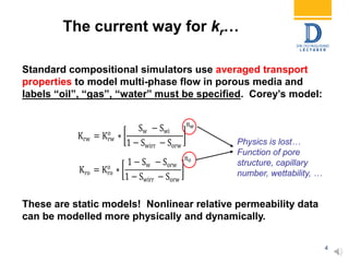
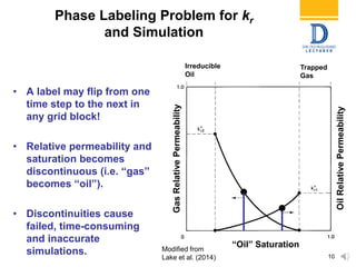
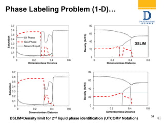
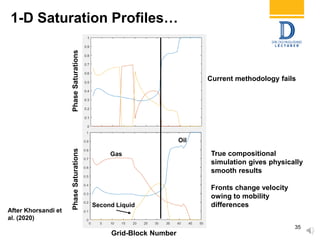
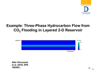
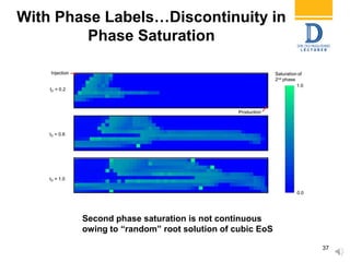
What are the advantages and disadvantages of membrane structures.pptx
Compositional Simulations that is Truly Compositional - Russell Johns
1. Primary funding is provided by
The SPE Foundation through member donations
and a contribution from Offshore Europe
The Society is grateful to those companies that allow their
professionals to serve as lecturers
Additional support provided by AIME
Society of Petroleum Engineers
Distinguished Lecturer Program
www.spe.org/dl
2. Compositional Simulation that is
Truly Compositional
Dr. Russell T. Johns
The Pennsylvania State University
George E. Trimble Chair in Earth and Mineral Sciences
rjohns@psu.edu
(44 Total Slides
Society of Petroleum Engineers
Distinguished Lecturer Program
www.spe.org/dl
3. 3
1) What defines a thermodynamic state function?
a) The function has one unique value for given input
parameters.
b) Integration of the function around a closed loop
yields zero.
c) The function change is independent of the path
taken.
2) Should petrophysical functions like relative permeability
(kr) have a unique (single) value for a given set of inputs
like saturation, phase connectivity, interfacial area,
anisotropic stress, capillary number, wettability, …?
3) Would it be useful that functions like kr and capillary
pressure (Pc) be coupled with similar inputs?
Quiz 1…
4. 4
Standard compositional simulators use averaged transport
properties to model multi-phase flow in porous media and
labels “oil”, “gas”, “water” must be specified. Corey’s model:
These are static models! Nonlinear relative permeability data
can be modelled more physically and dynamically.
Krw = Krw
o
∗
Sw − Swi
1 − Swirr − Sorw
𝑛 𝑤
Kro = Kro
o
∗
1 − Sw − Sorw
1 − Swirr − Sorw
𝑛 𝑜
Physics is lost…
Function of pore
structure, capillary
number, wettability, …
The current way for kr…
5. Quiz 2…
Why is relative permeability a function of phase labels, such as
oil, water, and gas?
Such labels began early on and worked well for water flooding
where oil and water are immiscible (distinguishable phases).
Relative permeabilities are measured with immiscible fluids as
functions only of labeled saturations.
Problem: Fluid properties change significantly during enhanced
oil recovery (EOR). Phase labels are meaningless!
5
6. 6
The Conventional-
Thinking Train is
Hard to Stop…
• Examples of old ways of
thinking are “barrels”
and labeling of phases
as “oil, gas, and water”.
• Using labeling can
change recoveries by up
to 20% OOIP from
simulation!
7. Outline
7
• What’s wrong with
compositional simulation?
• The fix is petrophysical!
• Incorporation of a new kr model
in compositional simulation
• Examples showing significant
benefits
• Conclusions
8. Is Compositional Simulation Truly
Compositional?
Compositional codes are not compositional, and owing to phase
labeling discontinuities are time consuming and can fail to converge.
8
Cubic EoS Flash
(T, P, composition)
Relative Permeability
(Labelled saturation)
Capillary Pressure
(Labelled saturation)
Grid to Grid Flux
Calculations
(Labelled saturation)
Current
Compositional
Simulators
Black-oil
simulation is
therefore used
most often owing
to its robustness.
9. Phase Labeling Example
• Consider a path from A
“gas” to B “oil” at fixed
composition.
• Labels input to kr curves:
krg = f(Sg) and kro = f(So).
• Problem: Where does the
phase label change and
can kr be continuous?
A
B
9
Pressure
TemperatureModified from
Lake et al. (2014)
10. Phase Labeling Problem for kr
and Simulation
• A label may flip from one
time step to the next in
any grid block!
• Relative permeability and
saturation becomes
discontinuous (i.e. “gas”
becomes “oil”).
• Discontinuities cause
failed, time-consuming
and inaccurate
simulations.
10“Oil” Saturation
GasRelativePermeability
OilRelativePermeability
Irreducible
Oil
Trapped
Gas
10
Modified from
Lake et al. (2014)
11. Objectives
Develop a unifying and predictive physical
approach to model rock-fluid interactions by
removing phase labels to improve robustness,
speed, and accuracy of compositional simulation
and give more reliable oil recovery estimates
11
12. New State Function (EoS) Approach to Model
Relative Permeability (kr)
Key References:
Khorsandi et al., 2016 (SPEJ)
Khorsandi et al. 2017 (SPE 182655)
Purswani et al. 2019 (Computational Geosciences)
Purswani et al. 2020 (SPE 200410)
12
13. 𝑘 𝑟 = 𝑓 𝑆, 𝜒, 𝐼, 𝑁𝑐, 𝜆 𝑑𝑘 𝑟 =
𝜕𝑘 𝑟
𝜕𝑆
𝑑S +
𝜕𝑘 𝑟
𝜕 𝜒
𝑑 𝜒 +
𝜕𝑘 𝑟
𝜕𝐼
𝑑𝐼 +
𝜕𝑘 𝑟
𝜕𝑁𝐶
𝑑𝑁𝐶 +
𝜕𝑘 𝑟
𝜕𝜆
𝑑𝜆
Gibbs energy is a state function that could depend on many
intensive and extensive parameters. We choose
Phase Euler connectivity index
Capillary number
(viscous/capillary)
Pore structure
Wettability index
(contact angle)
𝑘 𝑟 = S Φ − Φ 𝑟𝑒𝑓
Φ ≡ 𝑆 + 𝜒 = Flow function (no exponent!)
𝑑𝐺 =
𝜕𝐺
𝜕𝑃
𝑑𝑃 +
𝜕𝐺
𝜕𝑇
𝑑𝑇 +
𝑖=1
𝑛 𝑐
𝜕𝐺
𝜕𝑛𝑖
𝑑𝑛𝑖
New State Function (EoS) for kr
13
Similarly, relative permeability can be made a state function… If so,
this forces it to be continuous and unique, independent of labeling.
, , .iG f P T n
Saturation
Integration
14. Fluid Connectivity – A Little Topology
X = Euler Characteristic = # Pores – # Connections
14
X = 4 – 0 = 4X = 1 – 0 = 1X = 2 – 0 = 2X = 3 – 0 = 3
Four discontinuous
oil droplets
X = 4 – 1 = 3X = 4 – 2 = 2X = 4 – 3 = 1X = 4 – 4 = 0
All droplets are
continuous and
may flow
Smaller values of X
are more connected
Euler mentioned the formula in
his letter to Goldbach in 1750.
One pore filled
with oil
Oil is connected
between two pores
X = 4 – 5 = -1
15. 𝜒 = 167𝜒 = 87
Water image
Source of data: Chang et al. (2009). Environmental geology. 400 pores and nearly 760 possible
connections. Thus, 𝝌 𝒎𝒂𝒙 = 𝟒𝟎𝟎 and 𝝌 𝒎𝒊𝒏 = −𝟑𝟔𝟎.
Calculation of Euler Characteristic
(Khorsandi et al. 2017, SPEJ)
15
Normalized Connectivity
(Size independent)
𝜒 = 0 for fully 𝐝𝐢𝐬𝐜𝐨𝐧𝐧𝐞𝐜𝐭𝐞𝐝 phase
𝜒 = 1 for fully 𝐜𝐨𝐧𝐧𝐞𝐜𝐭𝐞𝐝 phase
Experimental Displacement Gas image
max
max min
ˆ
( 𝜒 = 0.41) ( 𝜒 = 0.31)
16. Source of data:
Chang et al. (2009). Environmental geology.
Drainage, 𝜒 = 0.74 Imbibition, 𝜒 = 0.63
16
Same saturation, but different relative permeability!
Impact of Euler Connectivity on kr
17. A Simple Thought Experiment…
17
Consider a porous rock at fixed capillary number and
pore structure:
The simplest model is constant partial derivatives:
How will kr change for an increase in S holding X and
wettability constant? Is the coefficient positive or
negative?
ˆˆ ,,cos ,cos
ˆ cos
ˆ cos
j jj j
rj rj rj
rj j j
j j S XX S
k k k
dk dS dX d
S X
ˆ cosrj S j X j I Sk S X
For increasing X with S and wettability constant?For increasing water wetness with X and S constant?
18. Relative Permeability Match to Data…
18
b
Excellent fit as a state function
with R2 = 0.971
ˆ
ˆ
j j
r j r j
j j j S
k k
S S
ˆ
j
r j
j S
k
ˆ
ˆ
j j
r j r j
j j j S
k k
S S
Nca ~ 10-4
Example data from
Armstrong et al. (2016)
Assuming saturation dependence
only, conventional Corey exponents
compensate, but predictability is lost
for other S-X paths.
Purswani et al. 2019 (Comp. Geo)
a
19. Illustration of Hysteresis (One Cycle)
19
Wetting-Phase Saturation (S)
Normalized(𝝌)
krw
1
3
2
Only one kr value
for given ( 𝝌 , S)!
See Purswani et
al. 2019, (Comp.
Geo.)
20. 0
0.2
0.4
0.6
0.8
1
0 0.2 0.4 0.6 0.8 1
kro
Non-Wetting Phase Saturation (𝑆 𝑜)
0
0.2
0.4
0.6
0.8
1
0 0.2 0.4 0.6 0.8 1
Pore Network Simulations for Oil-
Water Flow
20
• Bentheimer
sandstone
• 16,850 pores
After Purswani
et al. (2020,
SPE 200410)
First pore entered (𝜒=1)
Sor1
Residual
Locus
Sor2Sor3
Non-Wetting Phase Saturation (𝑆 𝑜)
Connectivity(𝜒𝑜)
kr equal to +- 0.01
Avg. contact angle 𝜃 ~ 50 𝑜
Path predictions:
• Imbibition
paths are
linear.
• Drainage
paths have
similar
curvature.
22. Best Fits to Experimental Data
22
• Unknown values
of 𝜒 determined
with d 𝝌 /dS = pSk.
• Fixed end-point
kr
o and S.
• kr-EoS fit data well
even at small
saturations.
After Purswani
et al. (2020, SPE
200410)
23. Data from Chang et al. (2009). Environmental Geology, “1” is drainage, “2” is imbibition..
𝑘 𝑟 = 𝑆 Φ − Φ 𝑟 Φ ≡ 𝑆 + 𝜒
Tuning with constant 𝑰, 𝑵 𝒄, 𝝀
Tuning of Micromodel Experiments
(See Khorsandi et al. 2017, SPEJ)
23
Prediction of krw
24. Impact of Capillary Number
24
a b
Slow increase in
connectivity
Fast increase in
connectivity
NCA ~ 1 (low IFT) NCA ~ 10-5 (high IFT)
ˆ
ˆ ˆ
j j
r j r j
j j j j S
k k
S S
ˆ
j
r j
j S
k
ˆ
j
r j
j j S
k
S
ˆ
ˆ ˆ
j j
r j r j
j j j j S
k k
S S
Corey exponent < 1
(Common for microemulsion phases that
form in surfactant polymer flooding)
Corey exponent > 1
𝜒
25. Truly Compositional Simulation…
1. Incorporate simple EoS for kr and Pc
2. Modify grid-block to grid-block phase flux
calculations. Flux occurs between phases
with most similar compositions.
Now, everything is truly compositional!
25
Phase 1
Phase 2
Phase 3
Grid block i Phase 2
Phase 1
Phase 3
Grid block i+1
26. Example: 1-D Continuous Injection Near
Critical Point (Ternary)
(Khorsandi et al. 2017, SPEJ)
26
27. kr
IMPECX Simulation of Miscible Flood
IMPECX ≡ Implicit Pressure Explicit Composition-
27
Solution is now continuous!
ˆX
Dimensionless Distance xDAfter Yuan and Pope, SPEJ, 2012
Gas
Oil
29. Surfactant Polymer Flooding and the Critical
Micelle Concentration (CMC)
(Khorsandi and Johns 2018, SPE 190207)
29
30. Effect of Critical Micelle Concentration
(CMC) on Relative Permeability
30
Optimum
Salinity
CMC
Phase labels change discontinuously from microemulsion phase to
oil/brine as Cs < CMC causing chemical simulation failures.
Very Low
Salinity
Low
Salinity
Very High
Salinity
High
Salinity
Microemulsion
phase
Brine phase
31. Chemical Simulation of
Layered Reservoir
31
Solutions are now continuous and there is no problem identifying
the microemulsion phase from excess oil/brine phases!
32. Oil Displacements by CO2 Resulting in Three-
Hydrocarbon Phases
(7-component oil, Okuno et al. 2010)
32
35. 1-D Saturation Profiles…
35
PhaseSaturations
Grid-Block Number
PhaseSaturations
Grid-Block Number
Current methodology fails
True compositional
simulation gives physically
smooth results
Fronts change velocity
owing to mobility
differences
After Khorsandi et
al. (2020)
Second Liquid
Oil
Gas
40. Results in Large Time-Step Sizes
and Unique Oil Recovery
40
Time-step sizes are near
the Courant–Friedrichs–
Lewy (CFL) limit.
max 1
u t
CFL
x
42. Conclusions
• Petrophysics is the solution to many reservoir engineering
problems! No more labeling even in modified black-oil
simulations!
• Physics-based EoS gives continuous rock-fluid properties
with changing S, , cos, Nc, and pore structure… Leads to
more accurate recovery estimates.
• Sor depends on the initial state in -S space and its path.
• There is improved convergence of flash calculations and
pressure solvers using the kr-EoS and grid-block flux
calculations… Leads to reduced computational time.
42
43. Acknowledgements…(rtj3@psu.edu)
Prior Students:
• Dr. Saeid Khorsandi (Chevron)
• Dr. Liwei Li (West Virginia U.)
• Dr. Ryosuke Okuno (UT-Austin)
• Dr. Meghdad Roshanfekr (BP)
• Mr. Prakash Purswani (Penn
State) 43
http://www.energy.psu.edu/gf/ George E. Trimble Chair
in EMS at Penn State
Editor's Notes
Additional comments
We would like to get a form similar to Broke and Corey
Corey’s model, all terms are zero
1- how this model is related to conventional models
2- There are many possible forms for relative permeability, one could actually define the coefficients in first equation and integrate them.
3- I affect other derivatives