This document describes a Ph.D. thesis that studied the seismic response of an instrumented multi-story reinforced concrete building in India. Acceleration time histories recorded in the building during the 2001 Bhuj earthquake are analyzed to determine modal parameters, floor accelerations and velocities, storey drifts, and other response quantities. Ambient vibration tests are conducted to identify the building's modal properties. Soil properties at the site are determined through in-situ and laboratory tests. Finite element models of the building with different levels of complexity are developed and analyzed under earthquake ground motions, both with and without considering soil-structure interaction effects. The observed and computed responses are then compared.


![xxiii
NOMENCLATURE
CHAPTER 3 - STRUCTURAL RESPONSE OF THE INSTRUMENTED
BUILDING FROM STRONG MOTION RECORD
EW East west direction
NS North south direction
Afloor Peak value of acceleration recorded at the concern floor level
AG Peak value of acceleration recorded at the ground floor level
NS1 First translational frequency in N-S direction
EW1 First translational frequency in E-W direction
T1 First torsional frequency
NS2 Second translational frequency in N-S direction
T2 Second torsional frequency
CHAPTER 4 - IDENTIFICATION OF MODAL PARAMETERS OF THE
INSTRUMENTED BUILDING FROM AMBIENT VIBRATION
RECORDS
t, τ Time
f Frequency
y(t) System response
,ϕ Mode shape, mode shape matrix
C Covariance matrix
G Spectral density matrix
u, U Singular vector, Matrix of singular vectors
[ ]is Diagonal matrix of singular values
CHAPTER 5- DETERMINATION OF INSITU SOIL PARAMETERS OF
FOUNDING SOIL OF THE INSTRUMENTED BUILDING
DS Disturbed soil sample
UDS Undisturbed soil sample
SPT Standard penetration test
SBC Safe bearing capacity
NP Non plastic
DST Direct shear test
LL Liquid limit
PL Plastic limit
PI Plasticity index](https://image.slidesharecdn.com/e06007d8-aa31-45d6-8e33-b25ea132ae82-150903142754-lva1-app6891/85/Complete-Thesis-29-320.jpg)


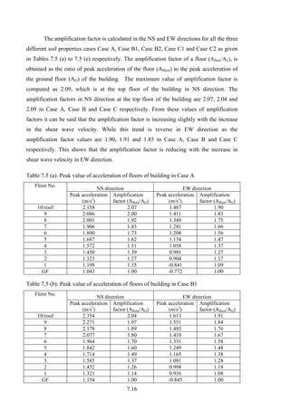
![3.27
3.13 whereas second mode is a torsional having natural frequency of 1.031 Hz. Detailed
study of different FE models of the building and their response to Bhuj earthquake have
been studied in Chapter 6 and 7.
Table 3.13: Modal frequencies of bare frame model
Mode M1 (Hz)
1 0.909 First translational mode in NS direction
2 1.031 First torsional mode
3 1.084 First translational mode in EW direction
4 1.582 Mixed mode
5 1.841 Mixed mode
3.7 ANALYSIS OF TIME HISTORIES FOR BUILDING RESPONSE, RESULT
AND DISCUSSION
3.7.1 Fourier Spectrum
A Fourier spectrum is a plot where Fourier amplitude (response of the linear
system) is extracted from the recorded signal, plotted against the frequencies of
excitation. Linear transforms, especially Fourier is widely used in solving problems in
science and engineering, which provides a link between the time domain and the
frequency domain of the signal. The Fourier transform is used in linear systems analysis
(Brigham, 1988). Although measurement data are usually available as samples of the
input and output time signals, it is very useful to look at the frequency-domain
representation of these signals. Many interesting signal’s features are revealed in
frequency domain. For instance, the Eigen frequencies of a structure emerge immediately
as the peaks in a frequency-domain plot of a measurement signal.
The mathematical tool to convert a time signal to the frequency domain is the
Fourier transform. Fourier transform of the accelerogram )(tx&& is given by Eq. (3.14).
∫
∞
∞−
ω−
=ω dtetxX ti
)()( && (3.14)
Assuming ground acceleration is non-zero in ],0( Tt ∈ the Eq. (3.14) can be written as](https://image.slidesharecdn.com/e06007d8-aa31-45d6-8e33-b25ea132ae82-150903142754-lva1-app6891/85/Complete-Thesis-77-320.jpg)


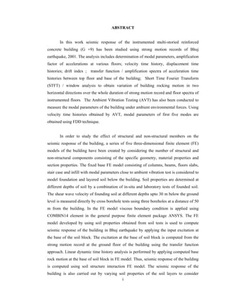
![3.32
record is obtained for the Ch.12 to Ch.8 by deducting the GF component of Ch.6. For
vertical component, Ch.14 is obtained by deducting Ch.13 from it.
The relative acceleration time histories obtained as described earlier have been
used as input for modal parameter extraction. Acceleration time history of the remaining
floors where there is no instrumental data is linearly interpolated. All floors are assumed
as rigid diaphragms and nodes where acceleration time histories are measured have been
considered as master nodes. The equations of other floor nodes have been obtained using
master nodes movement. To minimize the effect of noise in records, 200 SPS data is
decimated by a factor of two to have ultimate data of 100 SPS or having nyquist
frequency of 50Hz. Table 3.14 gives modal parameters of the instrumented building
based on strong motion records of Bhuj earthquake.
Table 3.14. Modal parameters estimated from strong motion data
Mode Frequency (Hz) Period (s) Damping Ratio (%)
1 1.26NS1
0.79 5.0
2 1.47EW1
0.68 2.9
3 2.34T1
0.43 2.7
4 3.91NS2
0.26 2.4
5 4.98T2
0.20 1.4
3.7.4 Short Time Fourier Transform (STFT)
In order to identify variation in the first two fundamental system frequencies over
the whole duration of earthquake, instantaneous system frequency was evaluated by
STFT as described in Trifunac et al. (2001). Apparent building rocking responses for the
EW and NS were evaluated as:
[ ] 30/)t(a)t(a)t( 712WE
..
−=θ − (3.22)
[ ] 30/)t(a)t(a)t( 16SN
..
−=θ − (3.23)
Where ai indicates the accelerations of sensor i and 30 is the building height in metre (see
Fig. 3.15 for sensor locations).](https://image.slidesharecdn.com/e06007d8-aa31-45d6-8e33-b25ea132ae82-150903142754-lva1-app6891/85/Complete-Thesis-82-320.jpg)


![4.7
Thus if the modal co-ordinates are un-correlated, the power spectral density matrix
( )fqqS of the modal co-ordinates is diagonal, and thus, if the mode shapes are orthogonal,
then Eq. (4.4) is a singular value decomposition (SVD) of the response spectral matrix.
Therefore, FDD is based on taking the SVD of the spectral density matrix
( ) ( )[ ] ( )T
iyy tsff UUG = (4.5)
The matrix [ ]...,u,uU 21= is a matrix of singular vectors and the matrix [ ]is is a diagonal
matrix of singular values. As it appears from this explanation, plotting the singular values
of the spectral density matrix will provide an overlaid plot of the auto spectral densities of
the modal coordinates. Note here that the singular matrix [ ]...,u,uU 21= is a function of
frequency because of the sorting process that is taking place as a part of the SVD
algorithm. A mode is identified by looking at where the first singular value has a peak, let
us say at the frequency 0f . This defines in the simplest form of the FDD technique - the
peak picking version of FDD - the modal frequency. The corresponding mode shape is
obtained as the corresponding first singular vector 1u in U .
( )01u f=ϕ (4.6)
For modal damping, enhanced FDD technique is used as described in Brincker et al.
(2000).
The modal damping is estimated using Enhanced FDD (EFDD) technique, which
is an extension to the FDD technique. In EFDD, the SDOF Power Spectral Density
function, identified around a resonance peak, is taken back to the time domain using the
Inverse Discrete Fourier Transform (IDFT). The damping is obtained by determining the
logarithmic decrement of the corresponding SDOF normalized auto correlation function.](https://image.slidesharecdn.com/e06007d8-aa31-45d6-8e33-b25ea132ae82-150903142754-lva1-app6891/85/Complete-Thesis-129-320.jpg)


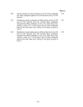
![5.7
5.4.1 Test Procedure
The boreholes, for conducting the cross borehole tests, had an internal diameter of
80 mm. and were made upto a depth of 30m below the natural ground level. These
boreholes were cased with PVC casing pipes and plugged at the bottom. PVC pipes
should withstand pressure upto 10kg/cm2
(IS: 4985 - 2000). The water inside the
boreholes was pumped out before conducting the test. Holes in alluvium soil close in
soon after digging and to prevent collapse or washouts, boreholes are normally cased with
plastic PVC pipe. The annular space between the casing and the surrounding soil has been
filled with 10 gallons of water per bag of cement, diluted with 5 to 10% bentonite by
volume [C., Doug, (2002)] to ensure a proper coupling of the soil with the borehole
casing.
A set of three boreholes laid out along a straight line, was used for conducting the
test as shown in Fig. 5.6. The spacing, centre to centre, between the first and second
boreholes was 4.88m and between the second and third boreholes it was 4.93m.
A schematic diagram of the cross borehole test setup is given in Fig.5.7. A Bison
borehole hammer was now lowered into the first borehole (borehole No. 1). This is a
special type of hammer with hydraulically operated shoes that can be extended or
retracted within the borehole as desired. At a predetermined depth, say 3.0m, the hammer
shoes were hydraulically extended to grip the borehole walls and lock the hammer in
place. Now two geophones were lowered into the other two boreholes (boreholes No. 2
and 3). These geophones with specially fitted rubber bladders, which can be inflated
pneumatically, can be locked in the borehole at any desired depth, 3.0m in this case. The
electrical signals from the borehole hammer and the geophones were fed into a Bison
seismograph (Fig. 5.8).
Having locked the borehole hammer and the geophones at the same desired depth,
3.0m in this case, the seismograph was switched on. A shear wave was now generated in
the first borehole by operating the hammer. This activated a timer switch in the
seismograph and the shear wave waveform arrivals at the borehole geophones were
displayed on the video screen of the seismograph. Figure 5.9 shows a typical record
obtained from the cross borehole test using superposition of waveforms and Fig. 5.10 shows](https://image.slidesharecdn.com/e06007d8-aa31-45d6-8e33-b25ea132ae82-150903142754-lva1-app6891/85/Complete-Thesis-157-320.jpg)


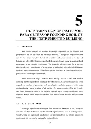
![6.6
6.4.1 Input excitation
Strong motion record at the ground floor in NS, EW and vertical directions of the
building is used as input excitation at the base of FE models for the dynamic time history
analysis. The frequency contents of input excitation in three perpendicular directions are
shown in Figs. 6.4 (a), 6.4 (b) and 6.4 (c). The characteristics of input excitation in three
perpendicular directions are given in Table 6.2.
Table 6.2: Characteristics of input excitation
Direction Peak acceleration
(m/s2
)
Time of occurrence of peak
acceleration (s)
NS 1.038 46.940
EW 0.782 34.945
Vertical 0.686 44.060
6.4.2 Material damping
The material damping of the reinforced concrete structure of the instrumented
multi-storied reinforced concrete building (G +9) is incorporated as Raleigh damping:
[ ] [ ] [ ]KMC β+α= (6.6)
Where α and β are Raleigh damping coefficients. The damping matrix [ ]C is orthogonal
with respect to system eigenvectors, and the modal damping coefficients Ci for the ith
mode may be calculated:
2
iiii 2C ωβ+α=ωξ= (6.7)
above equation (2) can be written in terms of modal critical ratio:
( ) 2/2/ iii ωβωαξ += (6.8)
The value of α and β are computed by using the first and second modal frequencies (i = 1,
2) with equation (3).
In the instrumented multi-storied reinforced concrete building (G +9) five percent
modal damping is observed in the first mode of the building in the earthquake from the
response of building to earthquake as described in Chapter 3. Therefore for the dynamic
time history analysis in the present study, five percent modal damping is considered for
the first two modes of the building to calculate values of α and β coefficients to](https://image.slidesharecdn.com/e06007d8-aa31-45d6-8e33-b25ea132ae82-150903142754-lva1-app6891/85/Complete-Thesis-178-320.jpg)


![7.10
7.7 MATERIAL DAMPING
The damping in the raft-soil-structure system includes material damping and the
radiation damping. The material damping has been incorporated as Raleigh damping:
[ ] [ ] [ ]KMC β+α= (5.1)
Where α and β are Raleigh damping coefficients. The damping matrix [ ]C is orthogonal
with respect to system eigenvectors, and the modal damping coefficients for the ith
mode
Ci may be calculated:
2
iiii 2C ωβ+α=ωξ= (5.2)
above equation (2) can be written in terms of modal critical ratio:
( ) 2/2/ iii ωβωαξ += (5.3)
The value of α and β are computed by using the first and second modal frequencies (i = 1,
2) with equation (3).
In the instrumented multi-storied reinforced concrete building (G +9) five percent
modal damping is observed in the first mode of the building during Bhuj earthquake as
mentioned in Chapter 3. Therefore for the dynamic time history analysis of building-raft-
soil system, five percent modal damping is considered for the first two modes to calculate
values of α and β coefficients to incorporate the Raleigh damping in the building-raft-soil
system. Material damping is assumed to be constant throughout the entire seismic event,
although the damping ratio varies with the strain level.
7.8 TYPE OF ANALYSIS PERFORMED ON THREE-DIMENSIONAL SOIL-
RAFT-BUILDING SYSTEM
Dynamic time history analysis has been performed using the comprehensive
building-raft-soil system. Input base excitation described in the next section, has been
applied at the bottom of the soil block in the FE model of the building for the whole
duration of the recorded Bhuj earthquake (133.525 s).](https://image.slidesharecdn.com/e06007d8-aa31-45d6-8e33-b25ea132ae82-150903142754-lva1-app6891/85/Complete-Thesis-208-320.jpg)