2. Since presidential elections only occur once every four years, it seems reasonable to assume the shocks
in will have dissipated by the time the next election occurs, which would make the error term in the
equation serially uncorrelated.
(ii) When the OLS residuals from
J = .481 −.0435JIJ H +.0544 JI +.0108JIJ H∙ J J -.0077JIJ H∙ J
(.012) (.0405) (.0234) (.0041) (.0033)
n=20, R2=.663, $ = .573
are regressed on the lagged residuals, we obtain = −.068 and J { { = .240. What do you conclude
about serial correlation in the ?
The t statistic is −.068 . 240 ≈ −.0283, which is very small, so the null H : = 0 is not rejected. The
value of −.068 for is also small which indicates serial correlation is not an issue.
(iii) Does the small sample size in this application worry you in testing for serial correlation?
The small sample size may be of some concern because the t statistic is only asymptotically justified.
But since the value for is both statistically insignificant and practically small, the usual OLS inference
procedures are usually not far off.
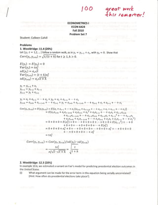
3. Wooldridge: C11.3 (20%)
(i) In Example 11.4, it may be that the expected value of the return at time t, given past returns,
is a quadratic function of J JJ # . To check this possibility, use the data in NYSE.RAW to
estimate
J JJ = + # J JJ # + $ J JJ # $ + ;
report the results in standard form.
J JJ = .2255486 +.0485723J JJ −1 −.009735J JJ −12
(.087234) (.0387224) (.0070296)
n=689, R2=.0063, $ = .0034
(ii) State and test the null hypothesis that {J JJ ÉJ JJ #{ does not depend on
J JJ # (Hint: there are two restrictions to test here. ) What do you conclude?
H : # = 0, $ =0
= 2.16
p-value: 0.1161
= 2.30 at the 10% significance level
Colleen Cahill ECON 6424 Problem Set 7 - 11/23/10 Page 2 of 7

3. With {É É = 2.16{ { = 2.30{ , and a p-value of .1161, there is insufficient evidence at the 10%
significance level to reject H : # = 0, $ = 0. We conclude J JJ # and J JJ # $ do not
have joint significance at the 10% level.
(iii) Drop J JJ # $ from the model, but add the interaction term J JJ # ∙ J JJ $.
Now test the efficient markets hypothesis.
J JJ = .1731605 +.0687116J JJ −1 +.0113384J JJ −1 ∙ J JJ −2
(.0809626) (.0392472) (.0100134)
n=688, R2=.0052, $ = .0023
H : # = 0, $ =0
= 1.80
p-value: 0.1658
= 2.30 at the 10% significance level
With {É É = 1.80{ { = 2.30{ , and a p-value of .1650, there is insufficient evidence at the 10%
significance level to reject H : # = 0, $ = 0. The p-value indicates we would not reject the null even
at 15% significance level. We conclude J JJ # and J JJ # ∙ J JJ $ do not have joint
significance at the 10% level.
(iv) What do you conclude about predicting weekly stock returns based on past stock returns?
It does not appear that weekly stock returns can be predicted based on past stock returns. Even using
the data from just one lag does not explain much of the variation in J JJ .
4. Wooldridge: C11.5 (20%)
(i) Add a linear time trend to the equation ∆ J = + # ∆J + $ ∆J # + % ∆J $ + . Is
a time trend necessary in the first-difference equation?
model: ∆ J= + # ∆J + $ ∆J # + % ∆J $ + +
∆ J= -1.267445 −.0348352∆J −.0131442∆J −1 +.11109∆J $ +.0078781
(1.046219) (.0272856) (.0278616) (.0272773) (.0242282)
n=69, R2=.2337, $ = .1859
.0078781
= = 0.33
.0242282
p-value: 0.746
= 1.96 at the 5% significance level for a two-tailed test
Colleen Cahill ECON 6424 Problem Set 7 - 11/23/10 Page 3 of 7

4. With {É É = 0.33{ { = 1.96{ , and a p-value of 0.746, there is insufficient evidence at the 5%
significance level to reject H : $ = 0 . We conclude is statistically insignificant (apparently very
much so with a p-value this large) and is not needed in the equation.
(ii) Drop the time trend and add the variables 2 and J to the equation (do not difference
these dummy variables). Are these variables jointly significant at the 5% level?
model: ∆ J= + # ∆J + $ ∆J # + % ∆J $ + 2+ 'J +
∆ J= -.6502546 −.0751636∆J −.0513865∆J # +.0882556∆J $ +4.839225 2 -1.676145J
(.5817652) (.0323566) (.0331632) (.0279766) (2.831973) (1.004766)
n=69, R2=.2956, $ = .2397
Test H : = 0, ' =0
F( 2, 63) = 2.82
Prob F = 0.0670
With {É É = 2.82{ { = 2.30{ , and a p-value of .0670, there is sufficient evidence at the 10%
significance level to reject H : = 0, ' = 0. The p-value indicates we would not reject the null at
the 5% significance level though. We conclude 2 and J have joint significance at the 10%
level.
(iii) Using the model from part (ii), estimate the LRP and obtain its standard error. Compare this
to
-22.13 2 −31.30J
J = 95.87 +.073J −.0058J +.034J # $
(3.28) (.126) (.1557) (.126) (10.73) (3.98)
n=70, R2=.499, $ = .459
where J and J appeared in levels rather than in first differences.
H = 1 + 2 + 3 = +.073 − .0058 + .034 ≈ .101
H = 1 + 2 + 3 = −.0751636 − .0513865 + .0882556 = −0.0382945
model: ∆ J= + # ∆J + $ {∆J # − ∆J { + % {∆J $ − ∆J { + 2+ 'J +
∆ J= -.6502546 −.0382945∆J −.0513865∆J # +.0882556∆J $ +4.839225 2 -1.676145J
(.5817652) (.0621577) (.0331632) (.0279766) (2.831973) (1.004766)
n=69, R2=.2956, $ = .2397
−.0382945
= = −.62
.0621577
Colleen Cahill ECON 6424 Problem Set 7 - 11/23/10 Page 4 of 7

5. p-value: 0.540
= 1.96 at the 5% significance level for a two-tailed test
With ? = .62C { = 1.96{ , and a p-value of .540, there is insufficient evidence at the 5%
significance level to reject H : # = 0 . We conclude the LRP is statistically insignificant at the 5%
level.
Compared with the LRP from the levels model, (which is positive and very significant) the LRP is now
negative and insignificant even at large significance levels.
5. Wooldridge: C12.5 (20%)
Consider the version of Fair’s model in Example 10.6. Now rather than predicting the
proportion of the two-party vote received by the Democrat, estimate a linear probability model
for whether or not the Democrat wins.
(i) Use the binary variable JJ in place of J in
J = + # JIJ H + $ JI + % JIJ H ∙ J J + JIJ H∙
J +
and report the results in standard form. Which factors affect the probability of
winning? Use the data only through 1992.
Model: JJ = + # JIJ H+ $ JI + % JIJ H∙ J J+
JIJ H∙ J +
JJ = .4405406 −.4730305JIJ H +.4792038 JI
(.1071623) (.353554) (.2046276)
+.0590304JIJ H∙ J J -.023867 JIJ H∙ J
(.0360612) (.0284591)
n=20, R2=.4371, $ = .2871
−.4730305
= = −1.34
.353554
p-value: 0.201
.4792038
= .2046276 = 2.34
p-value: 0.033
.0590304
JIJ H∙ J = .0360612 = 1.64
J
p-value: 0.122
−.023867
JIJ H∙ J = = −0.84
.0284591
p-value: 0.415
Colleen Cahill ECON 6424 Problem Set 7 - 11/23/10 Page 5 of 7

6. The only coefficient with a p-value low enough to be significant in a meaningful way is the one on
JI . But even that may be deceptive, for with an incumbent Democrat, the coefficient on JI
must be added to the coefficient on JIJ H, which nets out to zero.
The rest of the coefficients are less statistically significant, with the coefficient on JIJ H∙ J J
being the most significant. Even then it is not statistically significant until you reach above a 12%
significance level.
(ii) How many fitted values are less than zero? How many are greater than one?
Two of the fitted values are less than zero and two of the fitted values are greater than one.
(iii) Use the following prediction rule: if
JJ .5, you predict the Democrat wins;
otherwise, the Republican wins. Using this rule, determine how many of the 20
elections are correctly predicted by the model.
Of the 10 elections with JJ = 1, 8 of them are predicted correctly by the model.
Of the 10 elections with JJ = 0, 7 of them are predicted correctly by the model.
Therefore, 15 of the 20 elections are correctly predicted by the model.
(iv) Plug in the values of the explanatory variables for 1996. What is the predicted
probability that Clinton would win the election? Clinton did win; did you get the
correct prediction?
JJ = .4405406 − .473030{1{ + .4792038{1{ + .0590304{3{ − .023867{3.019{ = .5517507
Because . 5517507 .5, the model would predict Clinton winning, so the model predicted correctly.
(v) Use a heterskedasticity-robust test for AR(1) serial correlation in the errors. What
do you find?
Model: = + # # +
= -.0014714 −.1636607 −1
(.0867883) (.2057769)
n=20, R2=.0270
The correlation coefficient is ≈ −.1636607 with a t statistic using the robust standard
error of = −.1636607 . 2057769 = −0.80 and a p-value of 0.437, indicating serial
correlation does not appear to be a problem in the errors.
Colleen Cahill ECON 6424 Problem Set 7 - 11/23/10 Page 6 of 7

7. (vi) Obtain the heteroskedasticity-robust standard errors for the estimates in part (i).
Are there notable changes in any statistics?
JJ = .4405406 −.4730305JIJ H +.4792038 JI
(.1071623) (.353554) (.2046276)
[.0993785] [.3474566] [.2141727]
+.0590304JIJ H∙ J J -.023867 JIJ H∙ J
(.0360612) (.0284591)
[.0342501] [.0214536]
n=20, R2=.4371, $ = .2871
Usual se Robust se
−.4730305 −.4730305
= .353554 = −1.34 = .3474566 = −1.36
p-value: 0.201 p-value: 0.193
.4792038 .4792038
= .2046276 = 2.34 = .2141727 = 2.24
p-value: 0.033 p-value: 0.041
.0590304 .0590304
JIJ H∙ J = J = 1.64 JIJ H∙ J = J = 1.72
.0360612 .0342501
p-value: 0.122 p-value: 0.105
−.023867 −.023867
JIJ H∙ J= = −0.84 JIJ H∙ J = = −1.11
.0284591 .0214536
p-value: 0.415 p-value: 0.283
There is no change using the heteroskedasticity-robust standard errors that would make one of
the variables that much more significant than when using the usual standard errors. The
largest change is with JIJ H ∙ J which would become significant at a much lower significance
level than previously, but remains practically insignificant.
Colleen Cahill ECON 6424 Problem Set 7 - 11/23/10 Page 7 of 7