Relaibility

1. Chapter 7.0
RELIABILITY IN THE CONSTRUCTION OF
INFRASTRUCTURE PROJECTS

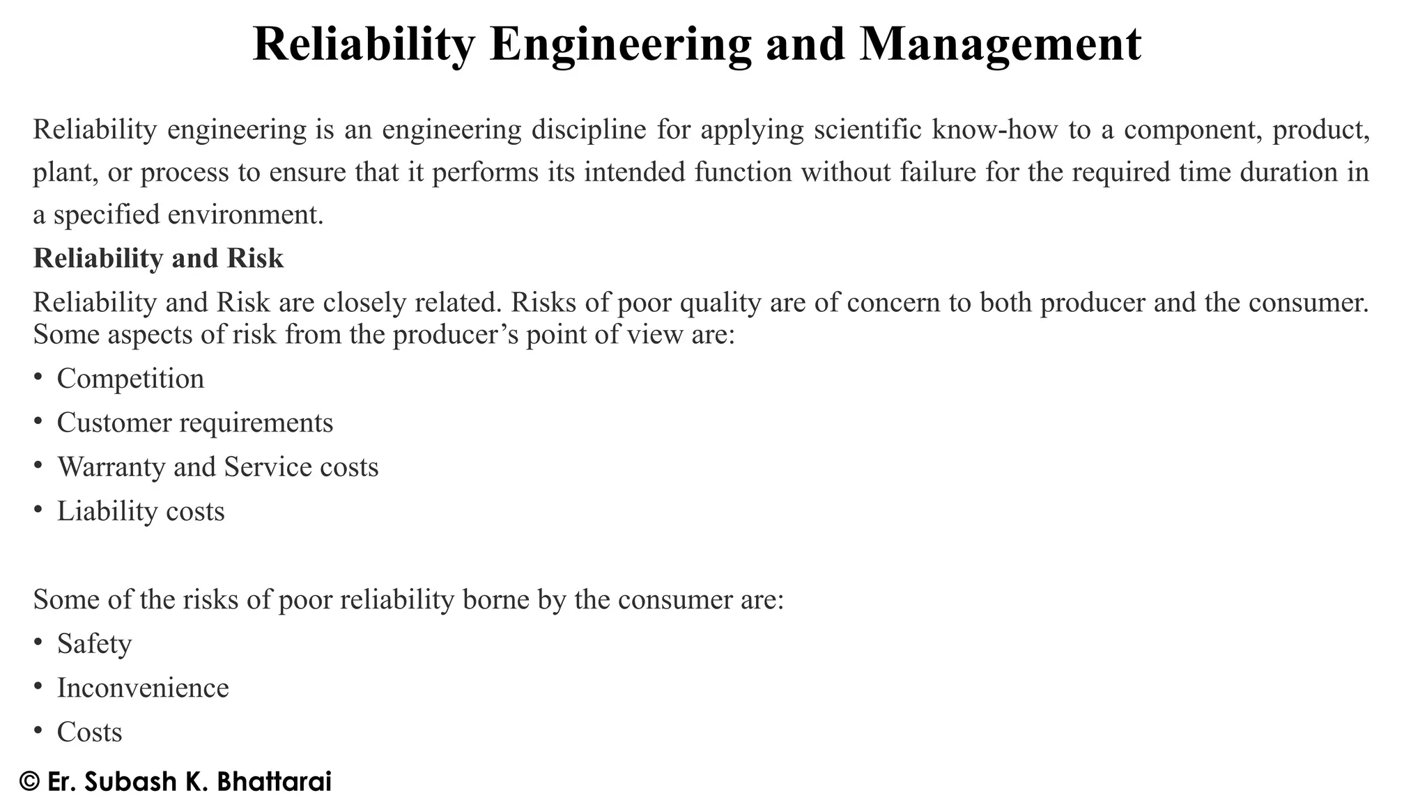
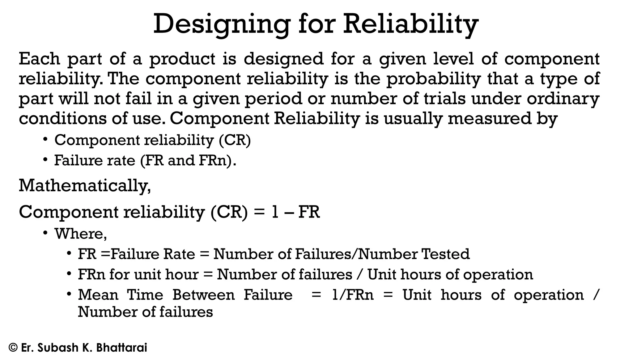
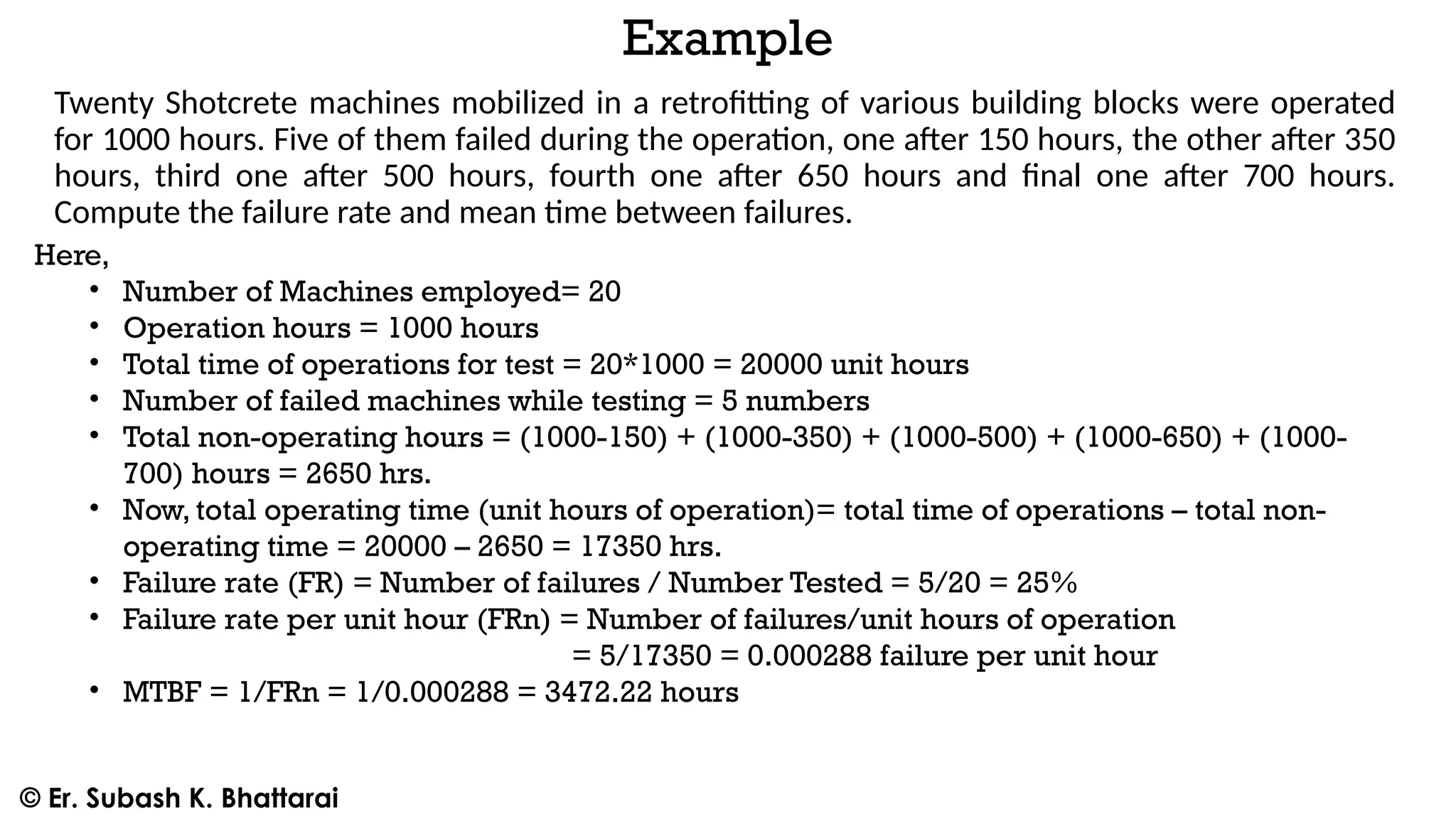
2. Reliability
Reliability is the likelihood that a component, equipment, or system performs
its intended function without failure over a specified time, under given
conditions.
In construction management, reliability refers to the consistent performance
of construction components or processes. For instance:
• A concrete batching plant operating without breakdown during a 30-day
highway paving operation.
• Structural formwork safely performing until removal without deformation or
collapse.
• A backup generator reliably supporting a hospital construction site during all
power outages over a 6-month period.

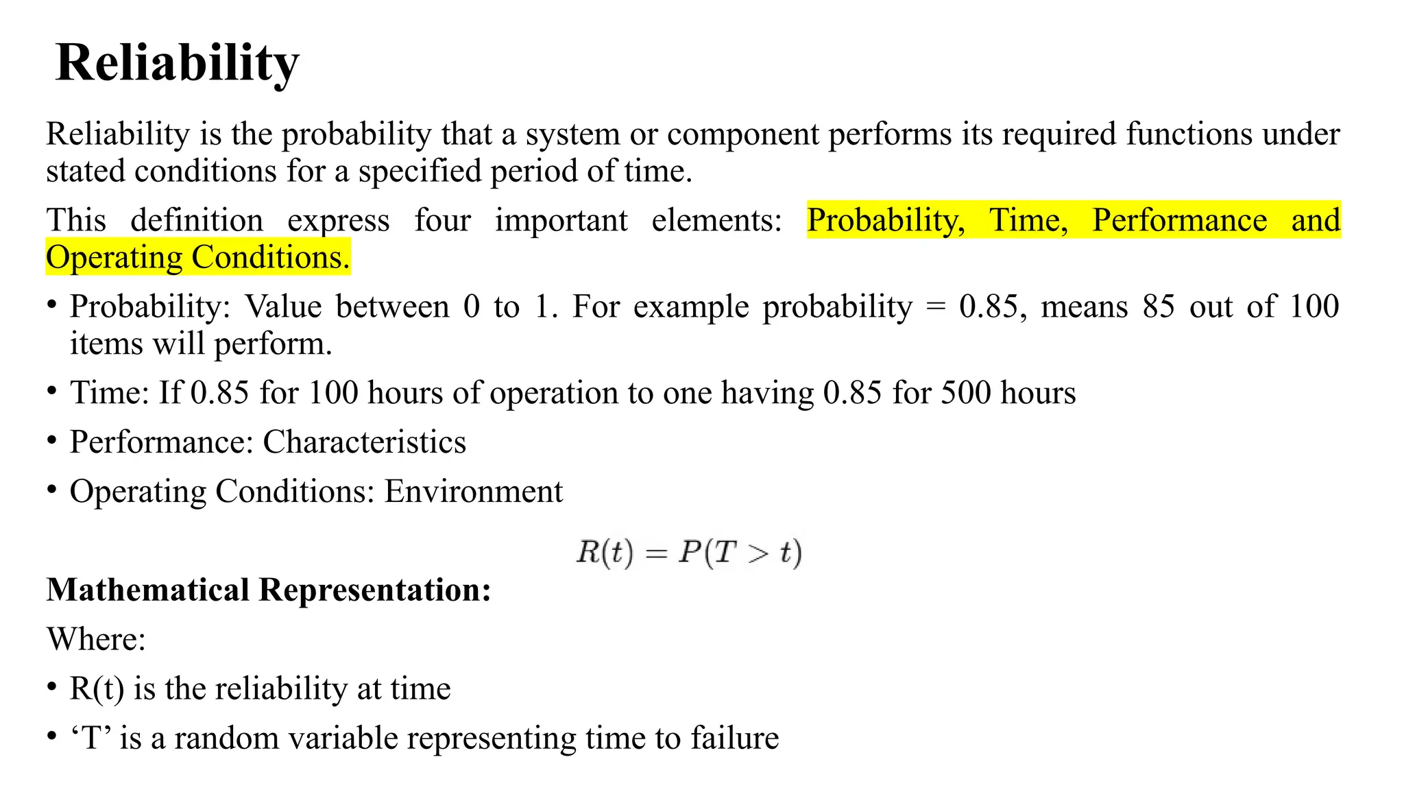
3. Reliability
Reliability is the probability that a system or component performs its required functions under
stated conditions for a specified period of time.
This definition express four important elements: Probability, Time, Performance and
Operating Conditions.
• Probability: Value between 0 to 1. For example probability = 0.85, means 85 out of 100
items will perform.
• Time: If 0.85 for 100 hours of operation to one having 0.85 for 500 hours
• Performance: Characteristics
• Operating Conditions: Environment
Mathematical Representation:
Where:
• R(t) is the reliability at time
• ‘T’ is a random variable representing time to failure

4. Reliability Engineering and Management
Reliability engineering is an engineering discipline for applying scientific know-how to a component, product,
plant, or process to ensure that it performs its intended function without failure for the required time duration in
a specified environment.
Reliability and Risk
Reliability and Risk are closely related. Risks of poor quality are of concern to both producer and the consumer.
Some aspects of risk from the producer’s point of view are:
• Competition
• Customer requirements
• Warranty and Service costs
• Liability costs
Some of the risks of poor reliability borne by the consumer are:
• Safety
• Inconvenience
• Costs
© Er. Subash K. Bhattarai

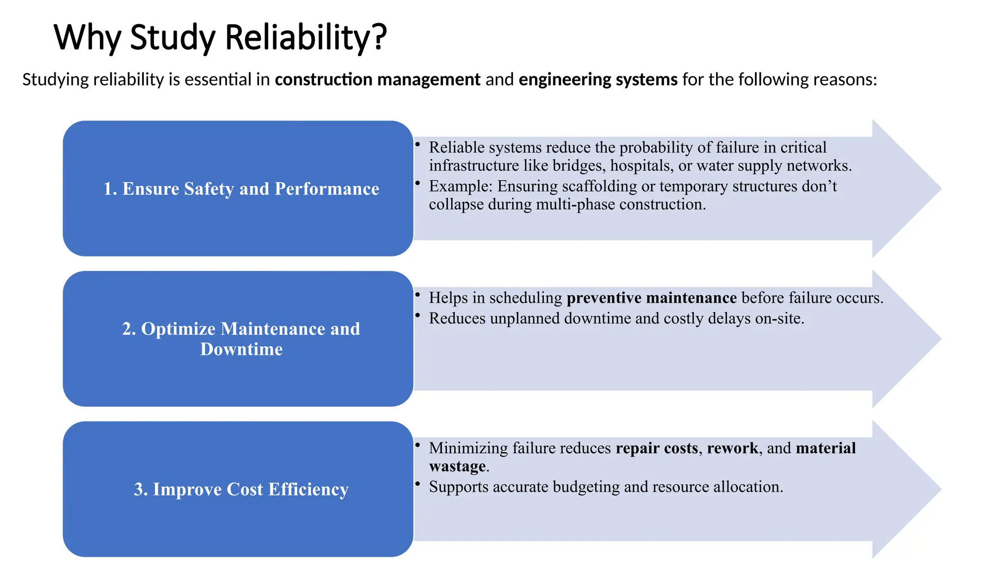
5. Why Study Reliability?
Studying reliability is essential in construction management and engineering systems for the following reasons:
• Reliable systems reduce the probability of failure in critical
infrastructure like bridges, hospitals, or water supply networks.
• Example: Ensuring scaffolding or temporary structures don’t
collapse during multi-phase construction.
1. Ensure Safety and Performance
• Helps in scheduling preventive maintenance before failure occurs.
• Reduces unplanned downtime and costly delays on-site.
2. Optimize Maintenance and
Downtime
• Minimizing failure reduces repair costs, rework, and material
wastage.
• Supports accurate budgeting and resource allocation.
3. Improve Cost Efficiency

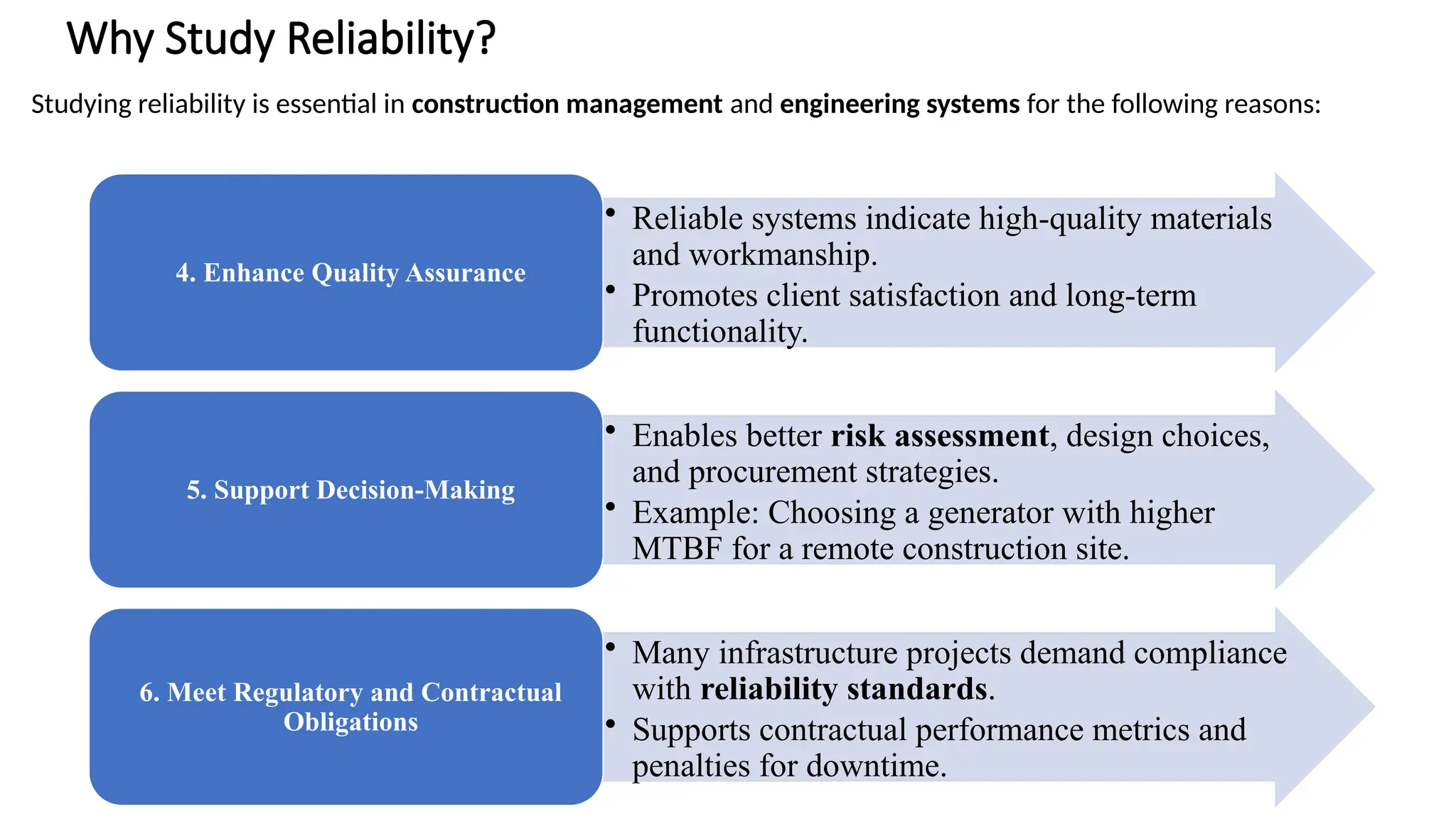
6. Why Study Reliability?
Studying reliability is essential in construction management and engineering systems for the following reasons:
• Reliable systems indicate high-quality materials
and workmanship.
• Promotes client satisfaction and long-term
functionality.
4. Enhance Quality Assurance
• Enables better risk assessment, design choices,
and procurement strategies.
• Example: Choosing a generator with higher
MTBF for a remote construction site.
5. Support Decision-Making
• Many infrastructure projects demand compliance
with reliability standards.
• Supports contractual performance metrics and
penalties for downtime.
6. Meet Regulatory and Contractual
Obligations

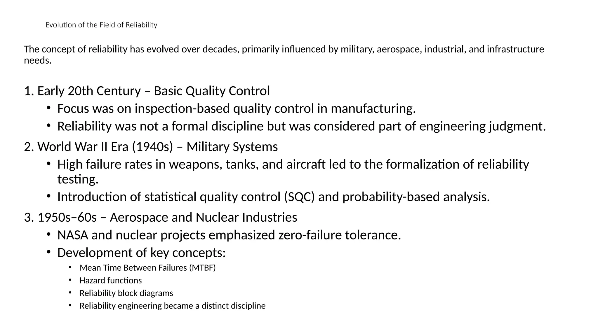
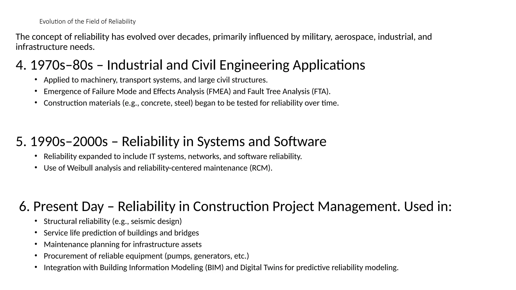
7. Evolution of the Field of Reliability
The concept of reliability has evolved over decades, primarily influenced by military, aerospace, industrial, and infrastructure
needs.
1. Early 20th Century – Basic Quality Control
• Focus was on inspection-based quality control in manufacturing.
• Reliability was not a formal discipline but was considered part of engineering judgment.
2. World War II Era (1940s) – Military Systems
• High failure rates in weapons, tanks, and aircraft led to the formalization of reliability
testing.
• Introduction of statistical quality control (SQC) and probability-based analysis.
3. 1950s–60s – Aerospace and Nuclear Industries
• NASA and nuclear projects emphasized zero-failure tolerance.
• Development of key concepts:
• Mean Time Between Failures (MTBF)
• Hazard functions
• Reliability block diagrams
• Reliability engineering became a distinct discipline.

8. Evolution of the Field of Reliability
The concept of reliability has evolved over decades, primarily influenced by military, aerospace, industrial, and
infrastructure needs.
4. 1970s–80s – Industrial and Civil Engineering Applications
• Applied to machinery, transport systems, and large civil structures.
• Emergence of Failure Mode and Effects Analysis (FMEA) and Fault Tree Analysis (FTA).
• Construction materials (e.g., concrete, steel) began to be tested for reliability over time.
5. 1990s–2000s – Reliability in Systems and Software
• Reliability expanded to include IT systems, networks, and software reliability.
• Use of Weibull analysis and reliability-centered maintenance (RCM).
6. Present Day – Reliability in Construction Project Management. Used in:
• Structural reliability (e.g., seismic design)
• Service life prediction of buildings and bridges
• Maintenance planning for infrastructure assets
• Procurement of reliable equipment (pumps, generators, etc.)
• Integration with Building Information Modeling (BIM) and Digital Twins for predictive reliability modeling.

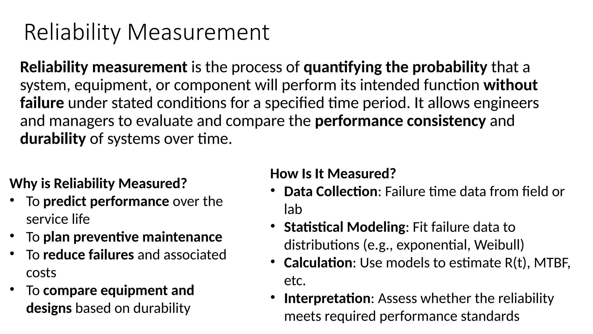
9. Reliability Measurement
Reliability measurement is the process of quantifying the probability that a
system, equipment, or component will perform its intended function without
failure under stated conditions for a specified time period. It allows engineers
and managers to evaluate and compare the performance consistency and
durability of systems over time.
Why is Reliability Measured?
• To predict performance over the
service life
• To plan preventive maintenance
• To reduce failures and associated
costs
• To compare equipment and
designs based on durability
How Is It Measured?
• Data Collection: Failure time data from field or
lab
• Statistical Modeling: Fit failure data to
distributions (e.g., exponential, Weibull)
• Calculation: Use models to estimate R(t), MTBF,
etc.
• Interpretation: Assess whether the reliability
meets required performance standards

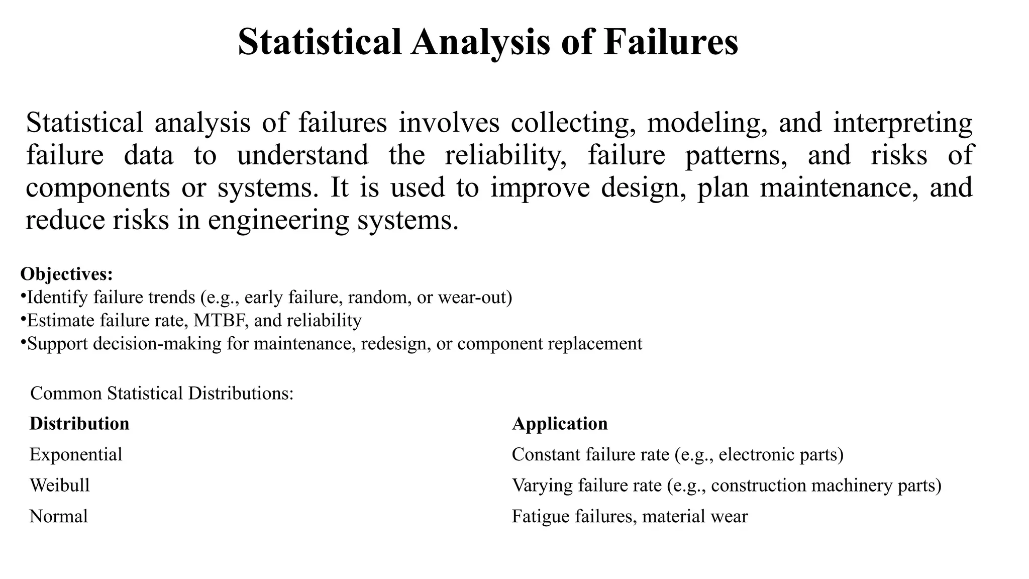
10. Statistical Analysis of Failures
Statistical analysis of failures involves collecting, modeling, and interpreting
failure data to understand the reliability, failure patterns, and risks of
components or systems. It is used to improve design, plan maintenance, and
reduce risks in engineering systems.
Objectives:
•Identify failure trends (e.g., early failure, random, or wear-out)
•Estimate failure rate, MTBF, and reliability
•Support decision-making for maintenance, redesign, or component replacement
Distribution Application
Exponential Constant failure rate (e.g., electronic parts)
Weibull Varying failure rate (e.g., construction machinery parts)
Normal Fatigue failures, material wear
Common Statistical Distributions:

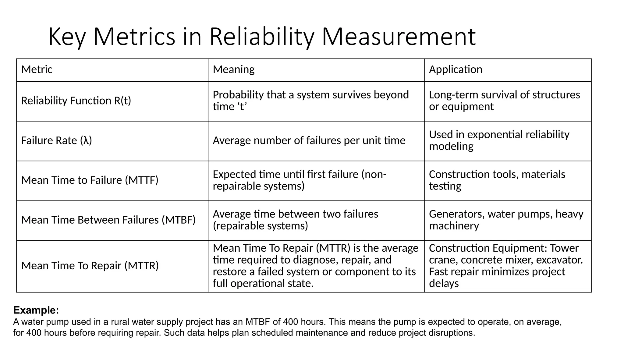
11. Key Metrics in Reliability Measurement
Metric Meaning Application
Reliability Function R(t)
Probability that a system survives beyond
time ‘t’
Long-term survival of structures
or equipment
Failure Rate (λ) Average number of failures per unit time
Used in exponential reliability
modeling
Mean Time to Failure (MTTF) Expected time until first failure (non-
repairable systems)
Construction tools, materials
testing
Mean Time Between Failures (MTBF)
Average time between two failures
(repairable systems)
Generators, water pumps, heavy
machinery
Mean Time To Repair (MTTR)
Mean Time To Repair (MTTR) is the average
time required to diagnose, repair, and
restore a failed system or component to its
full operational state.
Construction Equipment: Tower
crane, concrete mixer, excavator.
Fast repair minimizes project
delays
Example:
A water pump used in a rural water supply project has an MTBF of 400 hours. This means the pump is expected to operate, on average,
for 400 hours before requiring repair. Such data helps plan scheduled maintenance and reduce project disruptions.

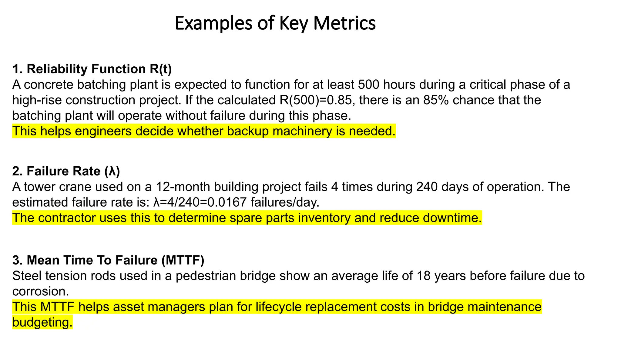
12. Examples of Key Metrics
1. Reliability Function R(t)
A concrete batching plant is expected to function for at least 500 hours during a critical phase of a
high-rise construction project. If the calculated R(500)=0.85, there is an 85% chance that the
batching plant will operate without failure during this phase.
This helps engineers decide whether backup machinery is needed.
2. Failure Rate (λ)
A tower crane used on a 12-month building project fails 4 times during 240 days of operation. The
estimated failure rate is: λ=4/240=0.0167 failures/day.
The contractor uses this to determine spare parts inventory and reduce downtime.
3. Mean Time To Failure (MTTF)
Steel tension rods used in a pedestrian bridge show an average life of 18 years before failure due to
corrosion.
This MTTF helps asset managers plan for lifecycle replacement costs in bridge maintenance
budgeting.

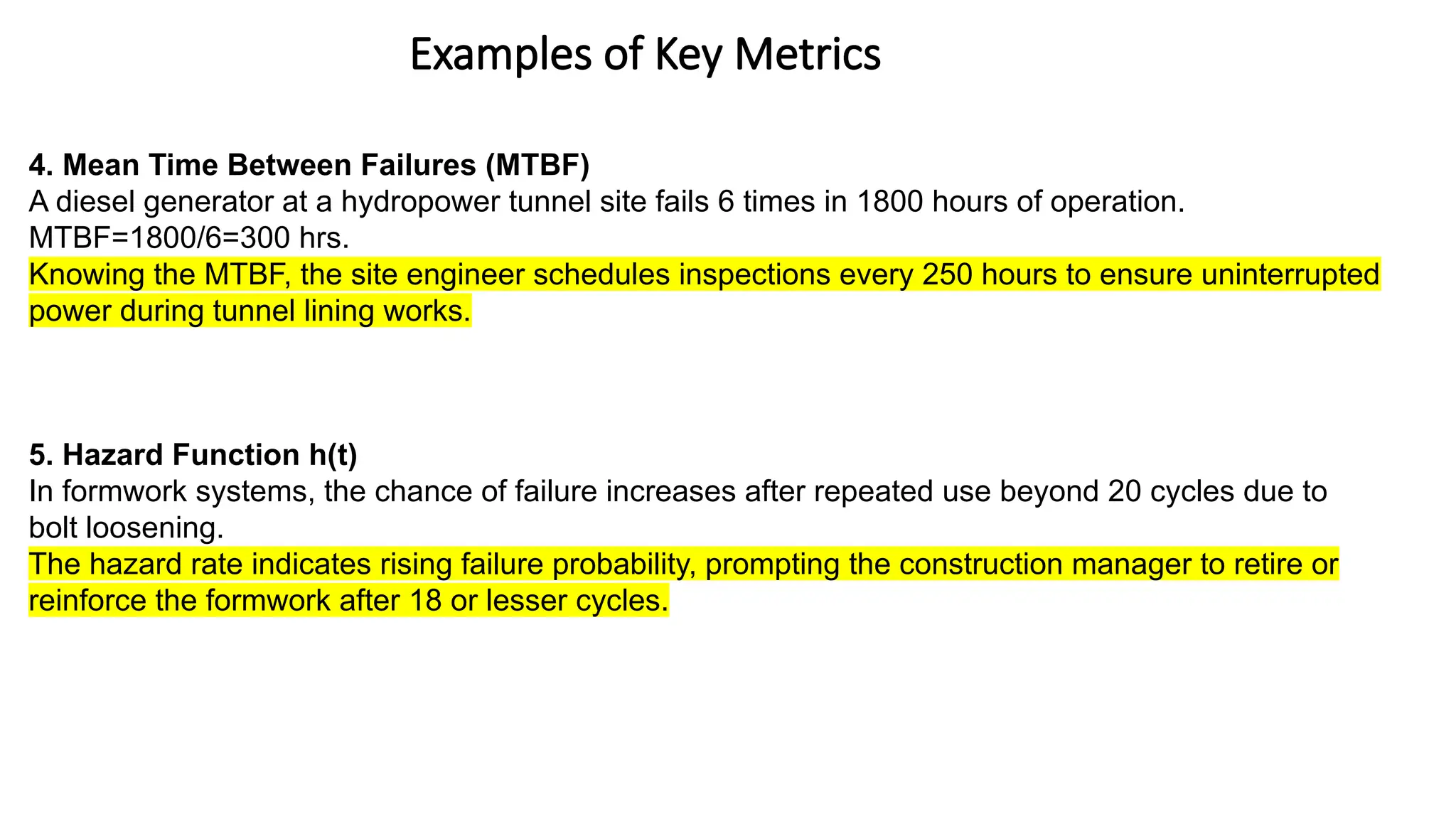
13. Examples of Key Metrics
4. Mean Time Between Failures (MTBF)
A diesel generator at a hydropower tunnel site fails 6 times in 1800 hours of operation.
MTBF=1800/6=300 hrs.
Knowing the MTBF, the site engineer schedules inspections every 250 hours to ensure uninterrupted
power during tunnel lining works.
5. Hazard Function h(t)
In formwork systems, the chance of failure increases after repeated use beyond 20 cycles due to
bolt loosening.
The hazard rate indicates rising failure probability, prompting the construction manager to retire or
reinforce the formwork after 18 or lesser cycles.

14. Designing for Reliability
Each part of a product is designed for a given level of component
reliability. The component reliability is the probability that a type of
part will not fail in a given period or number of trials under ordinary
conditions of use. Component Reliability is usually measured by
• Component reliability (CR)
• Failure rate (FR and FRn).
Mathematically,
Component reliability (CR) = 1 – FR
• Where,
• FR =Failure Rate = Number of Failures/Number Tested
• FRn for unit hour = Number of failures / Unit hours of operation
• Mean Time Between Failure = 1/FRn = Unit hours of operation /
Number of failures
© Er. Subash K. Bhattarai

15. Example
Twenty Shotcrete machines mobilized in a retrofitting of various building blocks were operated
for 1000 hours. Five of them failed during the operation, one after 150 hours, the other after 350
hours, third one after 500 hours, fourth one after 650 hours and final one after 700 hours.
Compute the failure rate and mean time between failures.
Here,
• Number of Machines employed= 20
• Operation hours = 1000 hours
• Total time of operations for test = 20*1000 = 20000 unit hours
• Number of failed machines while testing = 5 numbers
• Total non-operating hours = (1000-150) + (1000-350) + (1000-500) + (1000-650) + (1000-
700) hours = 2650 hrs.
• Now, total operating time (unit hours of operation)= total time of operations – total non-
operating time = 20000 – 2650 = 17350 hrs.
• Failure rate (FR) = Number of failures / Number Tested = 5/20 = 25%
• Failure rate per unit hour (FRn) = Number of failures/unit hours of operation
= 5/17350 = 0.000288 failure per unit hour
• MTBF = 1/FRn = 1/0.000288 = 3472.22 hours
© Er. Subash K. Bhattarai

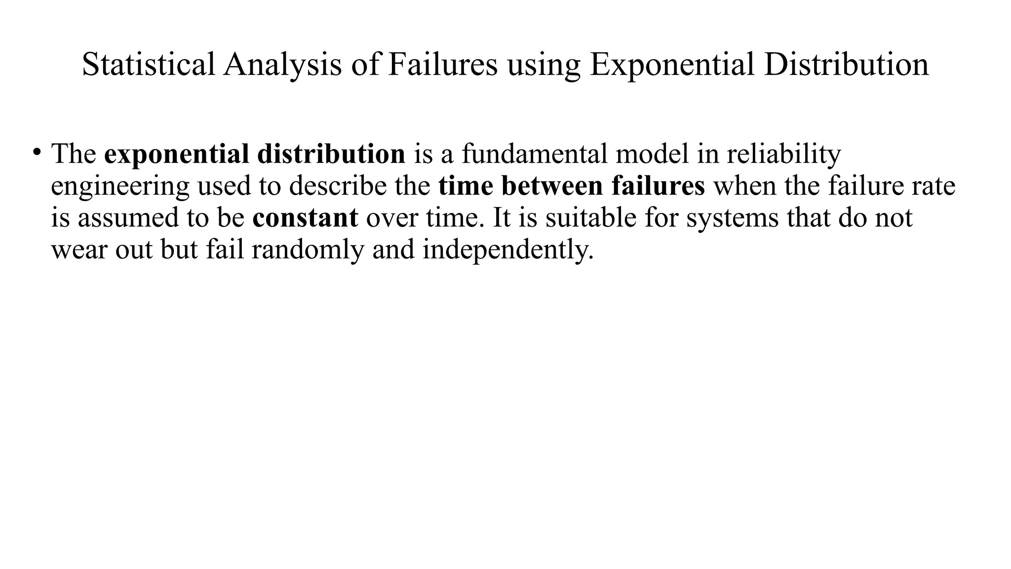
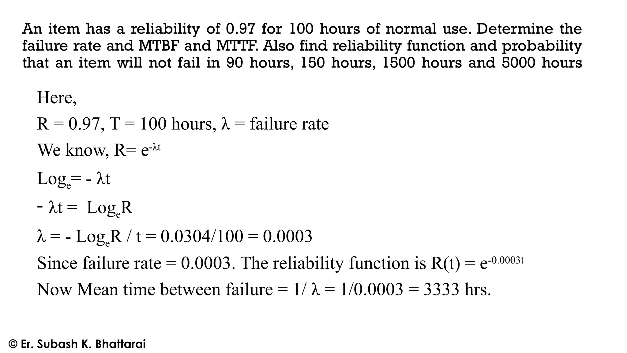
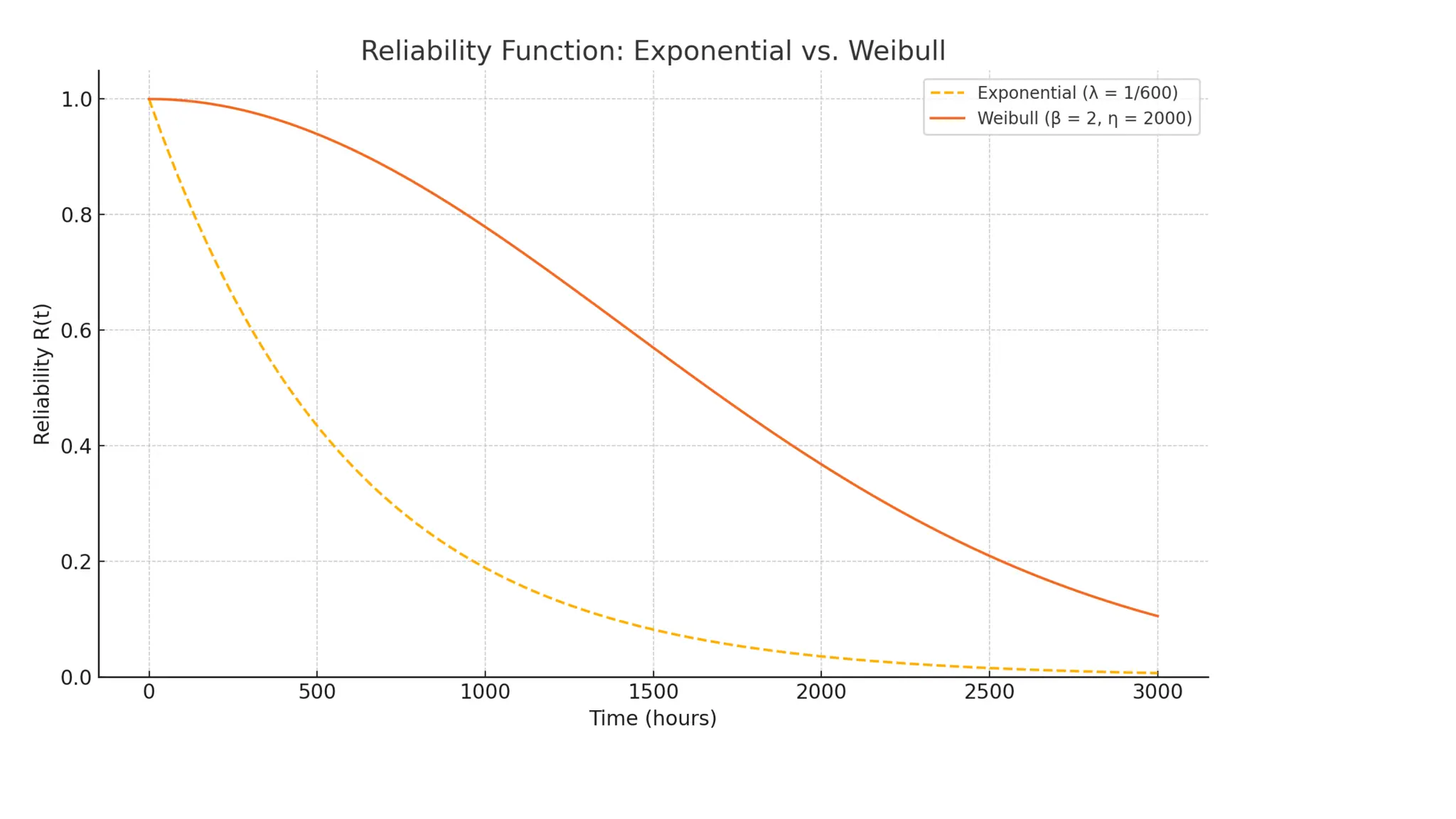
16. Statistical Analysis of Failures using Exponential Distribution
• The exponential distribution is a fundamental model in reliability
engineering used to describe the time between failures when the failure rate
is assumed to be constant over time. It is suitable for systems that do not
wear out but fail randomly and independently.

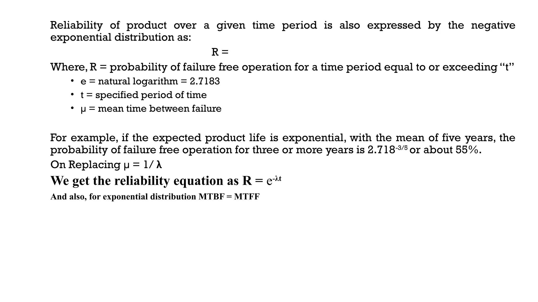
17. Reliability of product over a given time period is also expressed by the negative
exponential distribution as:
R =
Where, R = probability of failure free operation for a time period equal to or exceeding “t”
• e = natural logarithm = 2.7183
• t = specified period of time
• µ = mean time between failure
For example, if the expected product life is exponential, with the mean of five years, the
probability of failure free operation for three or more years is 2.718-3/5
or about 55%.
On Replacing µ = 1/ λ
We get the reliability equation as R = e-λt
And also, for exponential distribution MTBF = MTFF

18. An item has a reliability of 0.97 for 100 hours of normal use. Determine the
failure rate and MTBF and MTTF. Also find reliability function and probability
that an item will not fail in 90 hours, 150 hours, 1500 hours and 5000 hours
Here,
R = 0.97, T = 100 hours, λ = failure rate
We know, R= e-λt
Loge= - λt
- λt = LogeR
λ = - LogeR / t = 0.0304/100 = 0.0003
Since failure rate = 0.0003. The reliability function is R(t) = e-0.0003t
Now Mean time between failure = 1/ λ = 1/0.0003 = 3333 hrs.
© Er. Subash K. Bhattarai

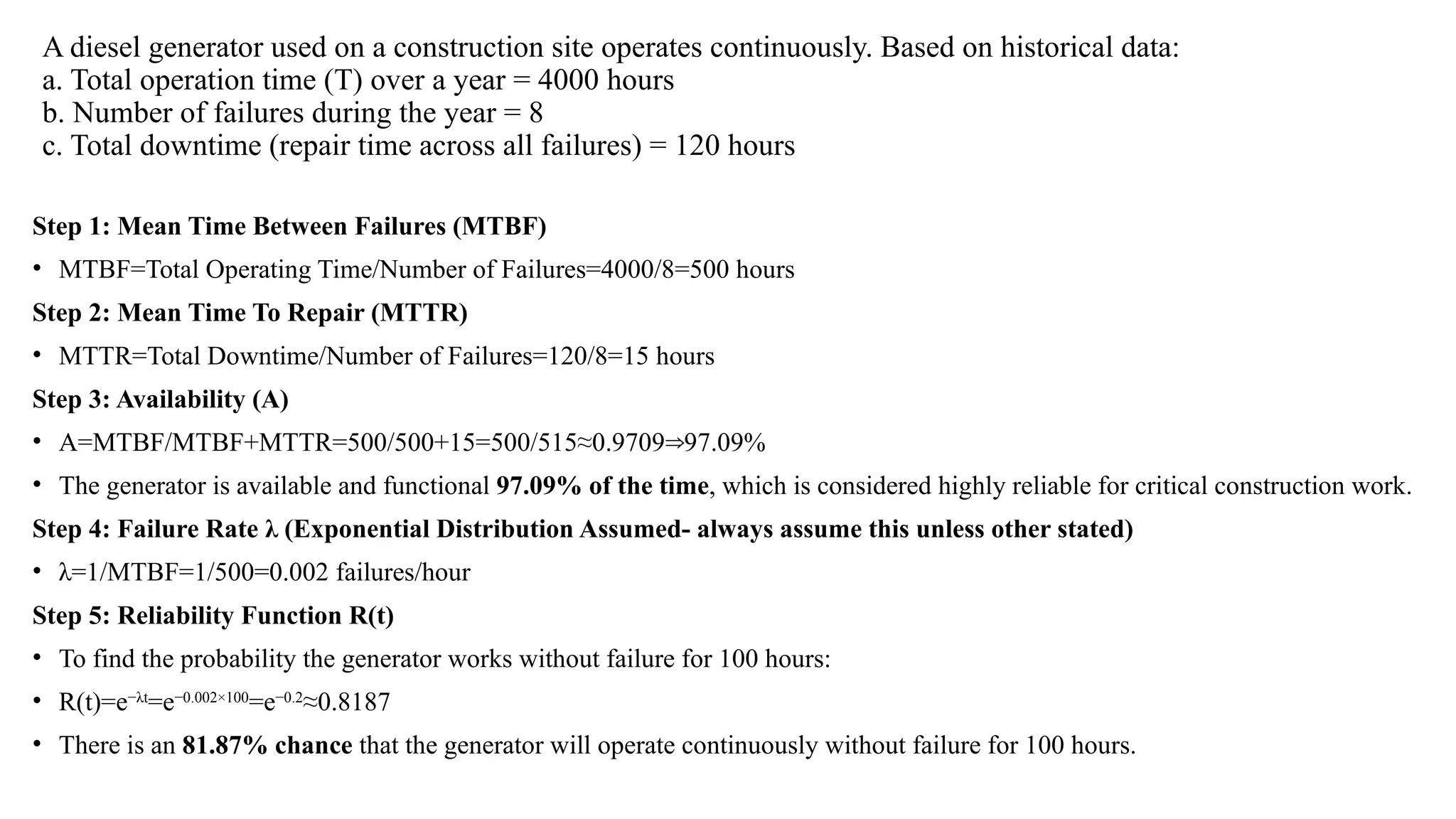
19. A diesel generator used on a construction site operates continuously. Based on historical data:
a. Total operation time (T) over a year = 4000 hours
b. Number of failures during the year = 8
c. Total downtime (repair time across all failures) = 120 hours
Step 1: Mean Time Between Failures (MTBF)
• MTBF=Total Operating Time/Number of Failures=4000/8=500 hours
Step 2: Mean Time To Repair (MTTR)
• MTTR=Total Downtime/Number of Failures=120/8=15 hours
Step 3: Availability (A)
• A=MTBF/MTBF+MTTR=500/500+15=500/515≈0.9709 97.09%
⇒
• The generator is available and functional 97.09% of the time, which is considered highly reliable for critical construction work.
Step 4: Failure Rate λ (Exponential Distribution Assumed- always assume this unless other stated)
• λ=1/MTBF=1/500=0.002 failures/hour
Step 5: Reliability Function R(t)
• To find the probability the generator works without failure for 100 hours:
• R(t)=e−λt
=e−0.002×100
=e−0.2
≈0.8187
• There is an 81.87% chance that the generator will operate continuously without failure for 100 hours.

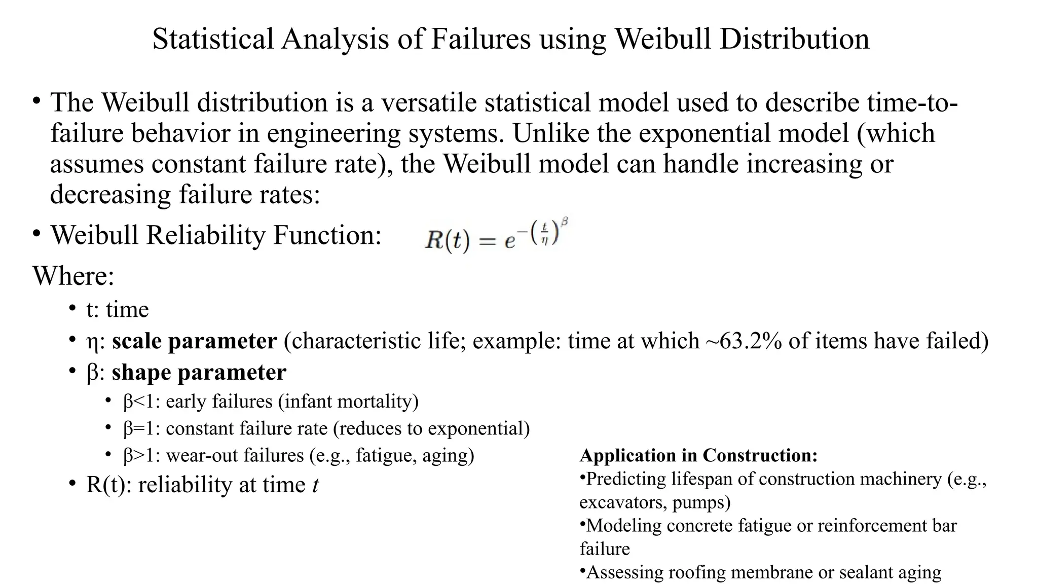
20. Statistical Analysis of Failures using Weibull Distribution
• The Weibull distribution is a versatile statistical model used to describe time-to-
failure behavior in engineering systems. Unlike the exponential model (which
assumes constant failure rate), the Weibull model can handle increasing or
decreasing failure rates:
• Weibull Reliability Function:
Where:
• t: time
• η: scale parameter (characteristic life; example: time at which ~63.2% of items have failed)
• β: shape parameter
• β<1: early failures (infant mortality)
• β=1: constant failure rate (reduces to exponential)
• β>1: wear-out failures (e.g., fatigue, aging)
• R(t): reliability at time t
Application in Construction:
•Predicting lifespan of construction machinery (e.g.,
excavators, pumps)
•Modeling concrete fatigue or reinforcement bar
failure
•Assessing roofing membrane or sealant aging

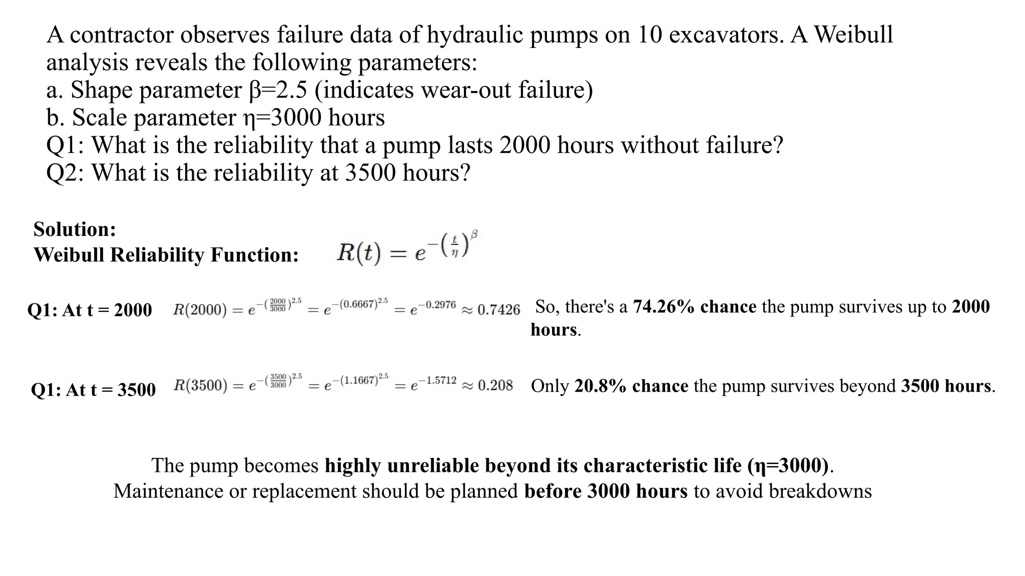
21. A contractor observes failure data of hydraulic pumps on 10 excavators. A Weibull
analysis reveals the following parameters:
a. Shape parameter β=2.5 (indicates wear-out failure)
b. Scale parameter η=3000 hours
Q1: What is the reliability that a pump lasts 2000 hours without failure?
Q2: What is the reliability at 3500 hours?
Solution:
Weibull Reliability Function:
Q1: At t = 2000 So, there's a 74.26% chance the pump survives up to 2000
hours.
Q1: At t = 3500 Only 20.8% chance the pump survives beyond 3500 hours.
The pump becomes highly unreliable beyond its characteristic life (η=3000).
Maintenance or replacement should be planned before 3000 hours to avoid breakdowns

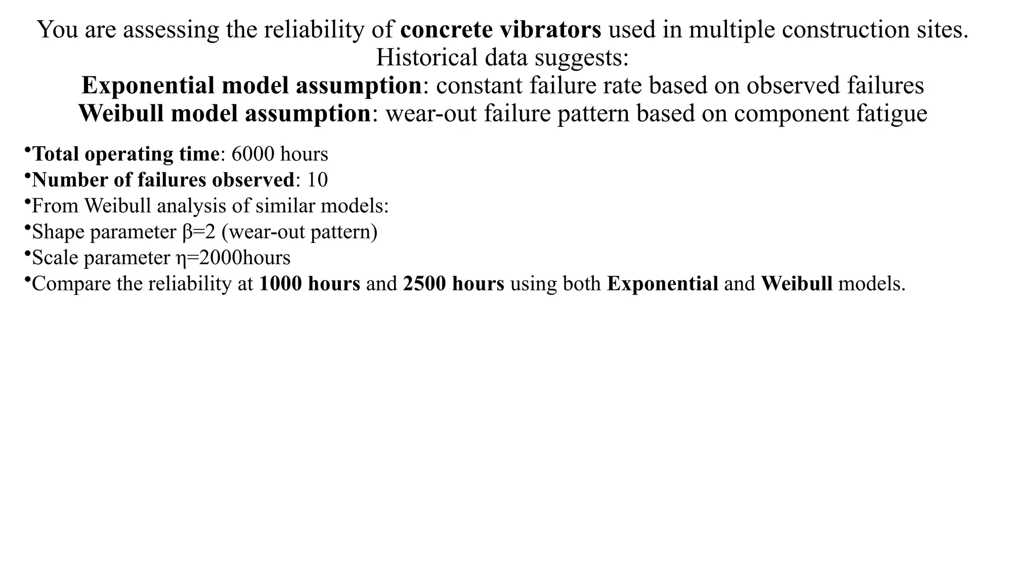
22. You are assessing the reliability of concrete vibrators used in multiple construction sites.
Historical data suggests:
Exponential model assumption: constant failure rate based on observed failures
Weibull model assumption: wear-out failure pattern based on component fatigue
•Total operating time: 6000 hours
•Number of failures observed: 10
•From Weibull analysis of similar models:
•Shape parameter β=2 (wear-out pattern)
•Scale parameter η=2000hours
•Compare the reliability at 1000 hours and 2500 hours using both Exponential and Weibull models.

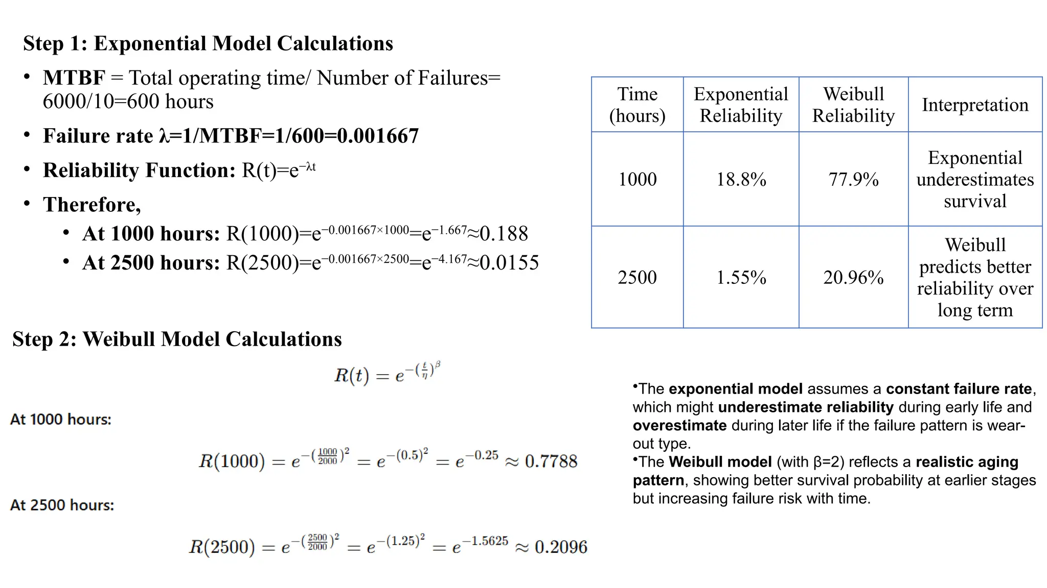
23. Step 1: Exponential Model Calculations
• MTBF = Total operating time/ Number of Failures=
6000/10=600 hours
• Failure rate λ=1/MTBF=1/600=0.001667
• Reliability Function: R(t)=e−λt
• Therefore,
• At 1000 hours: R(1000)=e−0.001667×1000
=e−1.667
≈0.188
• At 2500 hours: R(2500)=e−0.001667×2500
=e−4.167
≈0.0155
Step 2: Weibull Model Calculations
Time
(hours)
Exponential
Reliability
Weibull
Reliability
Interpretation
1000 18.8% 77.9%
Exponential
underestimates
survival
2500 1.55% 20.96%
Weibull
predicts better
reliability over
long term
•The exponential model assumes a constant failure rate,
which might underestimate reliability during early life and
overestimate during later life if the failure pattern is wear-
out type.
•The Weibull model (with β=2) reflects a realistic aging
pattern, showing better survival probability at earlier stages
but increasing failure risk with time.

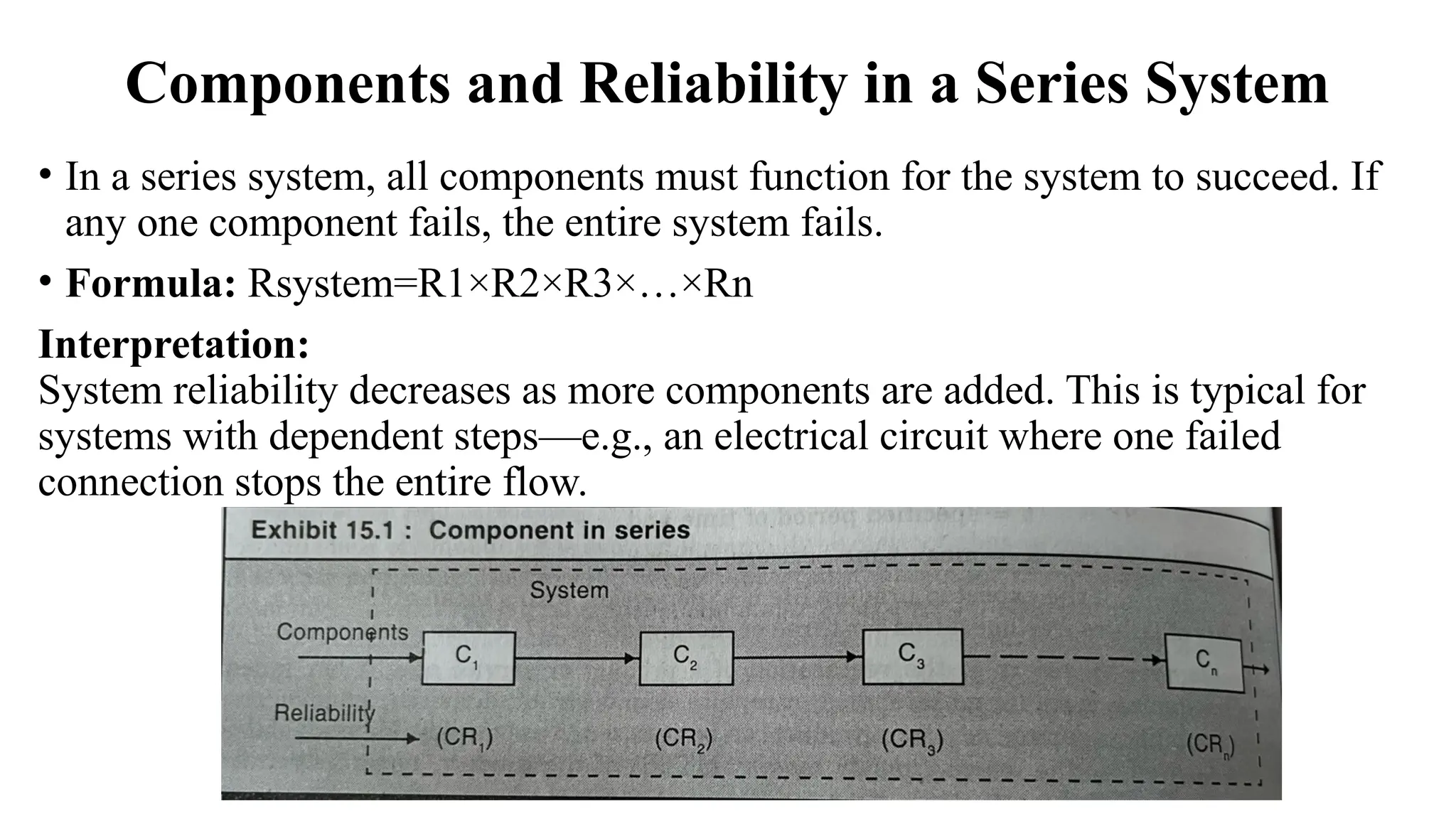
25. Components and Reliability in a Series System
• In a series system, all components must function for the system to succeed. If
any one component fails, the entire system fails.
• Formula: Rsystem=R1×R2×R3×…×Rn
Interpretation:
System reliability decreases as more components are added. This is typical for
systems with dependent steps—e.g., an electrical circuit where one failed
connection stops the entire flow.

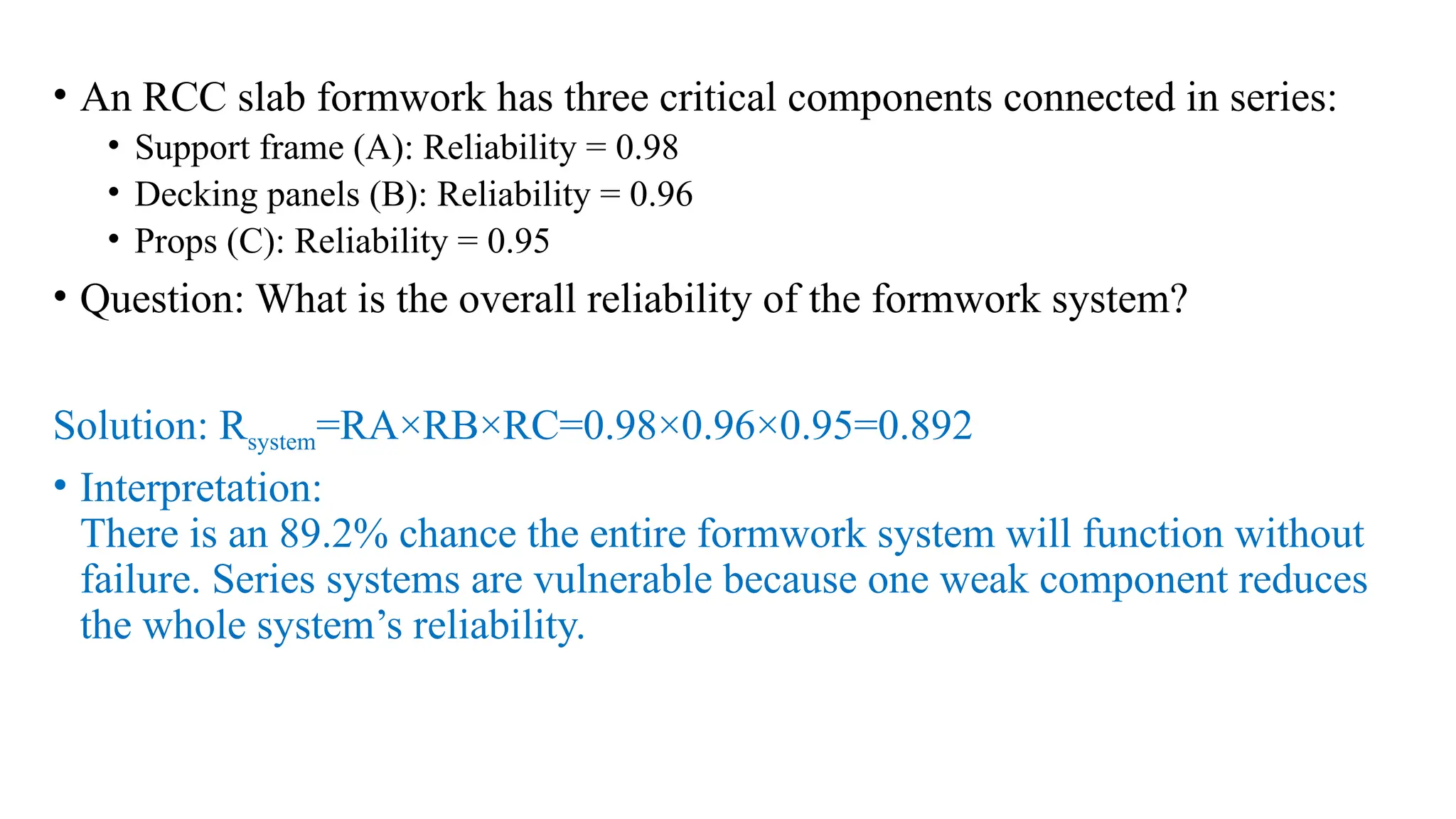
26. • An RCC slab formwork has three critical components connected in series:
• Support frame (A): Reliability = 0.98
• Decking panels (B): Reliability = 0.96
• Props (C): Reliability = 0.95
• Question: What is the overall reliability of the formwork system?
Solution: Rsystem=RA×RB×RC=0.98×0.96×0.95=0.892
• Interpretation:
There is an 89.2% chance the entire formwork system will function without
failure. Series systems are vulnerable because one weak component reduces
the whole system’s reliability.

27. Reliability in Parallel Systems
• Definition:
In a parallel system, the system works as long as at least one component
functions. All components must fail for the system to fail.
• Formula: Rsystem=1−[(1−R1)(1−R2)(1−R3)…(1−Rn)]
• Interpretation:
System reliability increases as more components are added in parallel. This
setup is used where redundancy is critical—e.g., backup power systems.

28. Problem:
A building’s water supply system has two pumps installed in parallel. Either
pump can independently serve the building. Their reliabilities are:
• Pump A: 0.85
• Pump B: 0.90
• Question: What is the overall system reliability?
Solution: Rsystem=1−[(1−RA)(1−RB)]=1−[(1−0.85)
(1−0.90)]=1−(0.15×0.10)=1−0.015=0.985
Interpretation:
The system has 98.5% reliability, showing that redundancy in parallel increases
system safety significantly.

29. Reliability in Mixed (Series-Parallel or Complex)
Systems
• Definition:
A mixed system combines both series and parallel configurations. The overall
reliability is calculated step-by-step, first solving for parallel or series subsections,
then combining them.
• Example Structure:
• Components A and B in parallel
• Combined result in series with component C
• RAB=1−[(1−RA)(1−RB)]
• Rsystem=RAB×RC
• Interpretation:
Mixed systems allow balancing between cost, complexity, and reliability, common
in construction (e.g., HVAC systems with backup blowers and series duct flow).

30. Problem:
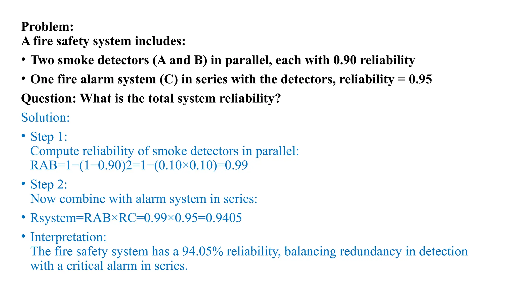
A fire safety system includes:
• Two smoke detectors (A and B) in parallel, each with 0.90 reliability
• One fire alarm system (C) in series with the detectors, reliability = 0.95
Question: What is the total system reliability?
Solution:
• Step 1:
Compute reliability of smoke detectors in parallel:
RAB=1−(1−0.90)2=1−(0.10×0.10)=0.99
• Step 2:
Now combine with alarm system in series:
• Rsystem=RAB×RC=0.99×0.95=0.9405
• Interpretation:
The fire safety system has a 94.05% reliability, balancing redundancy in detection
with a critical alarm in series.

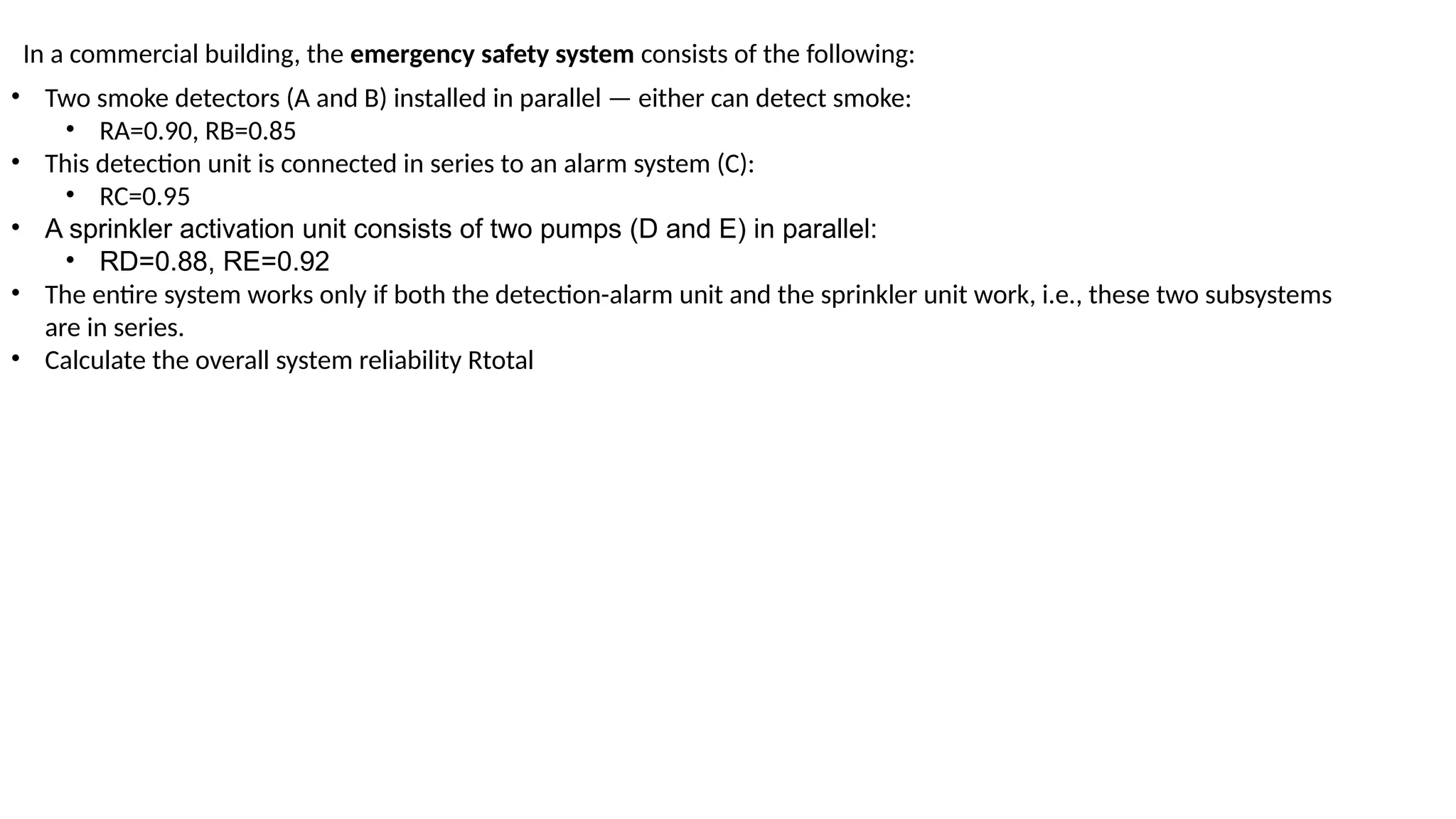
31. In a commercial building, the emergency safety system consists of the following:
• Two smoke detectors (A and B) installed in parallel — either can detect smoke:
• RA=0.90, RB=0.85
• This detection unit is connected in series to an alarm system (C):
• RC=0.95
• A sprinkler activation unit consists of two pumps (D and E) in parallel:
• RD=0.88, RE​
=0.92
• The entire system works only if both the detection-alarm unit and the sprinkler unit work, i.e., these two subsystems
are in series.
• Calculate the overall system reliability Rtotal

32. Solution
Step 1: Parallel Smoke Detectors (A and B)
• RAB=1−[(1−RA)(1−RB)]=1−[(1−0.90)
(1−0.85)]=1−(0.10×0.15)=1−0.015=0.985
Step 2: Detection + Alarm in Series (AB and C)
• RDetect+Alarm=RAB×RC=0.985×0.95=0.93575
Step 3: Parallel Sprinkler Pumps (D and E)
• RDE=1−[(1−RD)
(1−RE)]=1−(0.12×0.08)=1−0.0096=0.9904
Step 4: Total System Reliability (Detection+Alarm in
Series with Sprinkler Unit)
• Rtotal=(RDetect+Alarm)×RDE=0.93575×0.9904≈0.9268
The overall system reliability is 0.9268 or 92.68%