This document discusses procedures for testing claims and constructing confidence intervals about differences in two population proportions. Key points covered include:
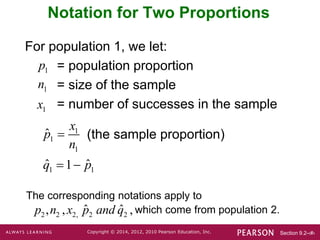
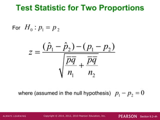
- How to test a claim about two population proportions using a z-test with the test statistic calculated as the difference between the sample proportions divided by the pooled standard error.
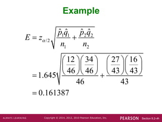
- How to construct a confidence interval for the difference between two population proportions using the pooled sample proportions and standard errors.
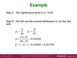
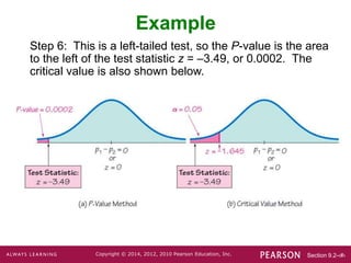
- An example that tests the claim that people are less likely to spend money given in large denominations by analyzing data on student spending behavior.