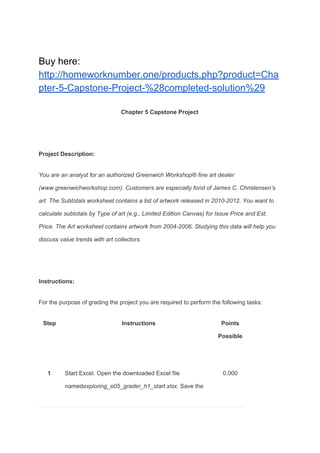
Buy here:
http://homeworknumber.one/products.php?product=Cha
pter-5-Capstone-Project-%28completed-solution%29
Chapter 5 Capstone Project
Project Description:
You are an analyst for an authorized Greenwich Workshop® fine art dealer
(www.greenwichworkshop.com). Customers are especially fond of James C. Christensen’s
art. The Subtotals worksheet contains a list of artwork released in 2010-2012. You want to
calculate subtotals by Type of art (e.g., Limited Edition Canvas) for Issue Price and Est.
Price. The Art worksheet contains artwork from 2004-2006. Studying this data will help you
discuss value trends with art collectors.
Instructions:
For the purpose of grading the project you are required to perform the following tasks:
Step Instructions Points
Possible
1 Start Excel. Open the downloaded Excel file
named​exploring_e05_grader_h1_start.xlsx​. Save the
0.000
workbook as​exploring_e05_grader_h1_LastFirst​,
replacing ​LastFirst​with your own name.
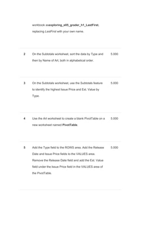
2 On the Subtotals worksheet, sort the data by Type and
then by Name of Art, both in alphabetical order.
5.000
3 On the Subtotals worksheet, use the Subtotals feature
to identify the highest Issue Price and Est. Value by
Type.
5.000
4 Use the Art worksheet to create a blank PivotTable on a
new worksheet named ​PivotTable​.
5.000
5 Add the Type field to the ROWS area. Add the Release
Date and Issue Price fields to the VALUES area.
Remove the Release Date field and add the Est. Value
field under the Issue Price field in the VALUES area of
the PivotTable.
5.000
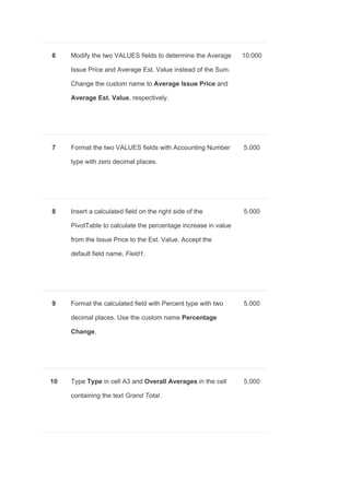
6 Modify the two VALUES fields to determine the Average
Issue Price and Average Est. Value instead of the Sum.
Change the custom name to ​Average Issue Price​and
Average Est. Value​, respectively.
10.000
7 Format the two VALUES fields with Accounting Number
type with zero decimal places.
5.000
8 Insert a calculated field on the right side of the
PivotTable to calculate the percentage increase in value
from the Issue Price to the Est. Value. Accept the
default field name, ​Field1​.
5.000
9 Format the calculated field with Percent type with two
decimal places. Use the custom name ​Percentage
Change​.
5.000
10 Type ​Type​in cell A3 and ​Overall Averages​in the cell
containing the text​Grand Total​.
5.000
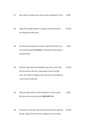
11 Set a filter to display only sold-out art (indicated by ​Yes​). 5.000
12 Apply Pivot Style Medium 5, display banded columns,
and display banded rows.
10.000
13 Use the Art worksheet to create a blank PivotChart on a
new sheet named ​PivotChart​. Change the chart type to
Clustered Bar.
5.000
14 Add the Type field to the ROWS area of the chart. Add
the Issue Price and Est. Value fields to the VALUES
area. Set a filter to display only sold-out art (indicated by
Yes) for the PivotChart.
10.000
15 Hide the field buttons in the PivotChart. Insert a chart
title above the chart and type ​2005-2007 Art​.
5.000
16 Format the value axis with Accounting with zero decimal
places. Apply 8-pt size to the category axis and value
10.000
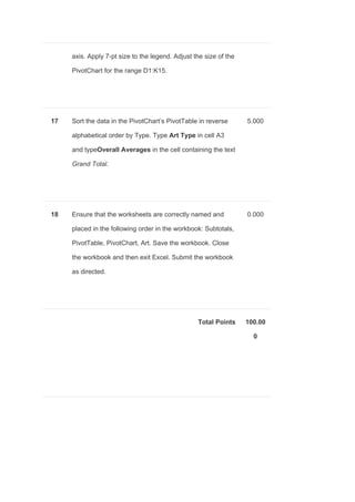
axis. Apply 7-pt size to the legend. Adjust the size of the
PivotChart for the range D1:K15.
17 Sort the data in the PivotChart’s PivotTable in reverse
alphabetical order by Type. Type ​Art Type​in cell A3
and type​Overall Averages​in the cell containing the text
Grand Total​.
5.000
18 Ensure that the worksheets are correctly named and
placed in the following order in the workbook: Subtotals,
PivotTable, PivotChart, Art. Save the workbook. Close
the workbook and then exit Excel. Submit the workbook
as directed.
0.000
Total Points 100.00
0

Chapter 5 Capstone Project (completed solution)

  • 1.
    Buy here: http://homeworknumber.one/products.php?product=Cha pter-5-Capstone-Project-%28completed-solution%29 Chapter 5Capstone Project Project Description: You are an analyst for an authorized Greenwich Workshop® fine art dealer (www.greenwichworkshop.com). Customers are especially fond of James C. Christensen’s art. The Subtotals worksheet contains a list of artwork released in 2010-2012. You want to calculate subtotals by Type of art (e.g., Limited Edition Canvas) for Issue Price and Est. Price. The Art worksheet contains artwork from 2004-2006. Studying this data will help you discuss value trends with art collectors. Instructions: For the purpose of grading the project you are required to perform the following tasks: Step Instructions Points Possible 1 Start Excel. Open the downloaded Excel file named​exploring_e05_grader_h1_start.xlsx​. Save the 0.000
  • 2.
    workbook as​exploring_e05_grader_h1_LastFirst​, replacing ​LastFirst​withyour own name. 2 On the Subtotals worksheet, sort the data by Type and then by Name of Art, both in alphabetical order. 5.000 3 On the Subtotals worksheet, use the Subtotals feature to identify the highest Issue Price and Est. Value by Type. 5.000 4 Use the Art worksheet to create a blank PivotTable on a new worksheet named ​PivotTable​. 5.000 5 Add the Type field to the ROWS area. Add the Release Date and Issue Price fields to the VALUES area. Remove the Release Date field and add the Est. Value field under the Issue Price field in the VALUES area of the PivotTable. 5.000
  • 3.
    6 Modify thetwo VALUES fields to determine the Average Issue Price and Average Est. Value instead of the Sum. Change the custom name to ​Average Issue Price​and Average Est. Value​, respectively. 10.000 7 Format the two VALUES fields with Accounting Number type with zero decimal places. 5.000 8 Insert a calculated field on the right side of the PivotTable to calculate the percentage increase in value from the Issue Price to the Est. Value. Accept the default field name, ​Field1​. 5.000 9 Format the calculated field with Percent type with two decimal places. Use the custom name ​Percentage Change​. 5.000 10 Type ​Type​in cell A3 and ​Overall Averages​in the cell containing the text​Grand Total​. 5.000
  • 4.
    11 Set afilter to display only sold-out art (indicated by ​Yes​). 5.000 12 Apply Pivot Style Medium 5, display banded columns, and display banded rows. 10.000 13 Use the Art worksheet to create a blank PivotChart on a new sheet named ​PivotChart​. Change the chart type to Clustered Bar. 5.000 14 Add the Type field to the ROWS area of the chart. Add the Issue Price and Est. Value fields to the VALUES area. Set a filter to display only sold-out art (indicated by Yes) for the PivotChart. 10.000 15 Hide the field buttons in the PivotChart. Insert a chart title above the chart and type ​2005-2007 Art​. 5.000 16 Format the value axis with Accounting with zero decimal places. Apply 8-pt size to the category axis and value 10.000
  • 5.
    axis. Apply 7-ptsize to the legend. Adjust the size of the PivotChart for the range D1:K15. 17 Sort the data in the PivotChart’s PivotTable in reverse alphabetical order by Type. Type ​Art Type​in cell A3 and type​Overall Averages​in the cell containing the text Grand Total​. 5.000 18 Ensure that the worksheets are correctly named and placed in the following order in the workbook: Subtotals, PivotTable, PivotChart, Art. Save the workbook. Close the workbook and then exit Excel. Submit the workbook as directed. 0.000 Total Points 100.00 0