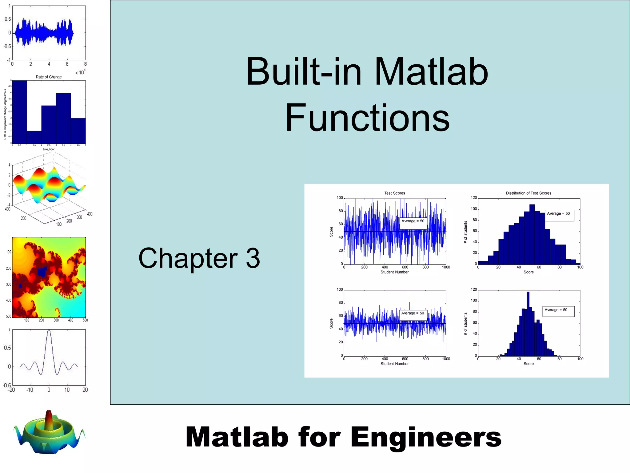
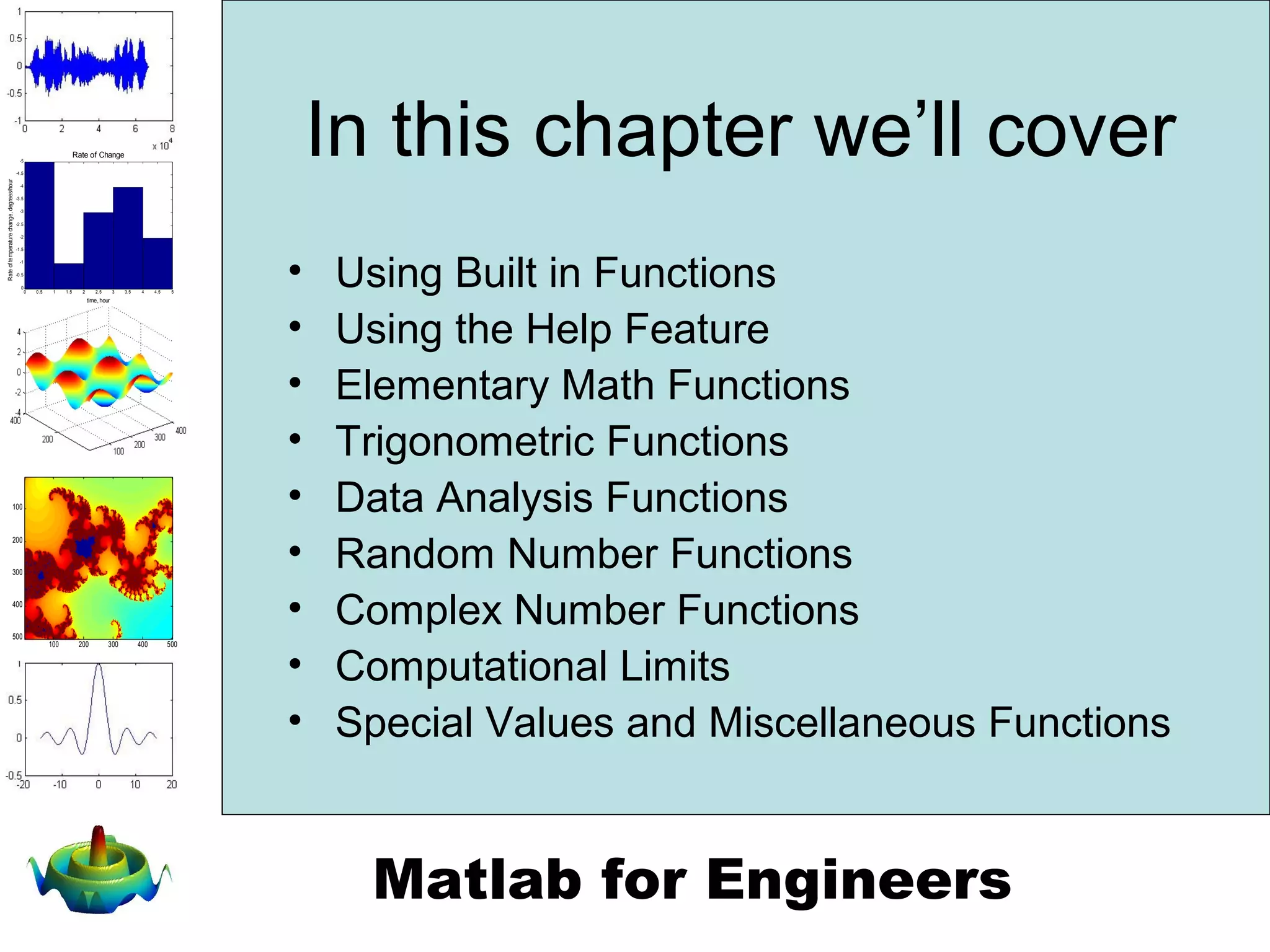
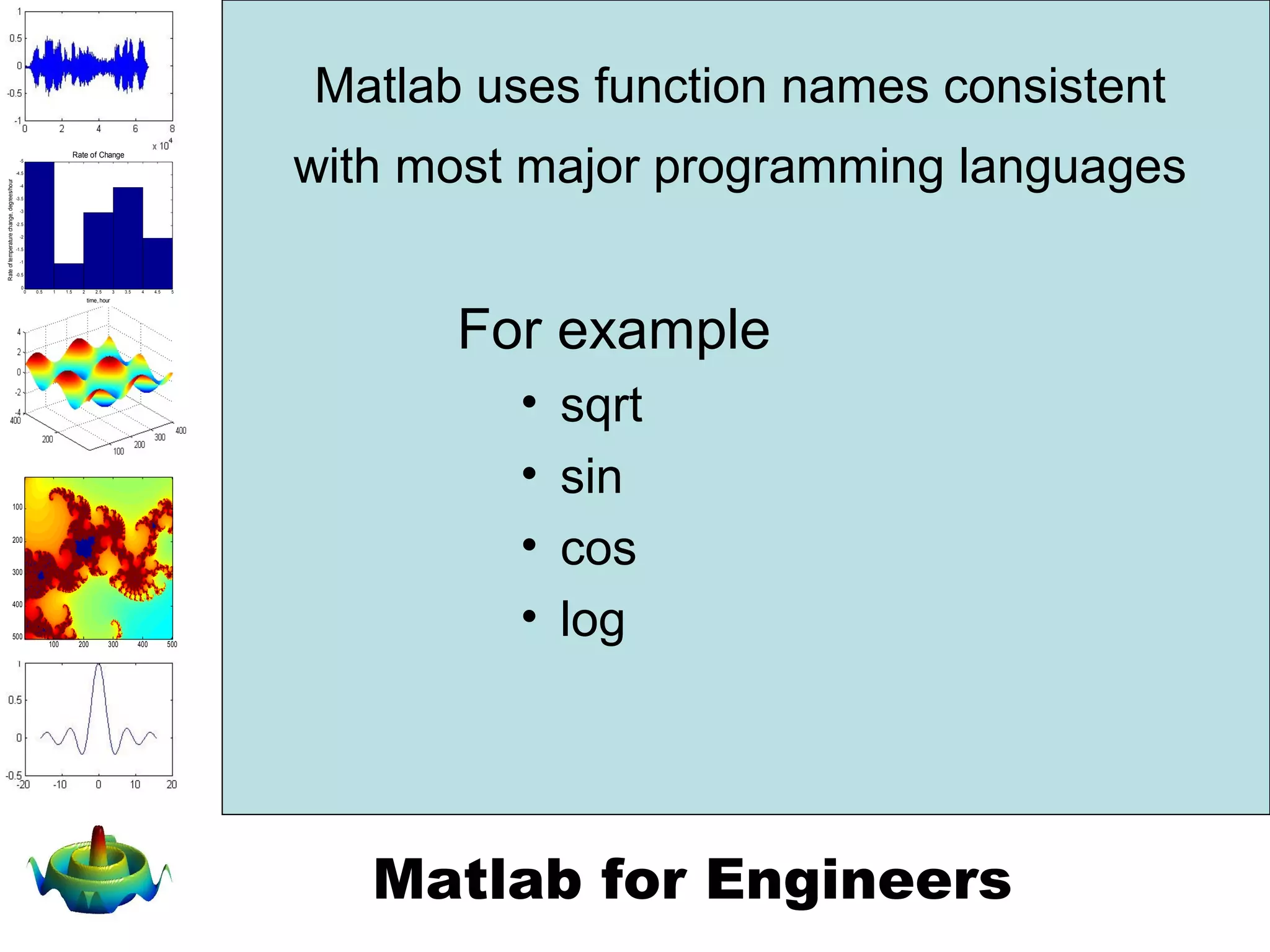
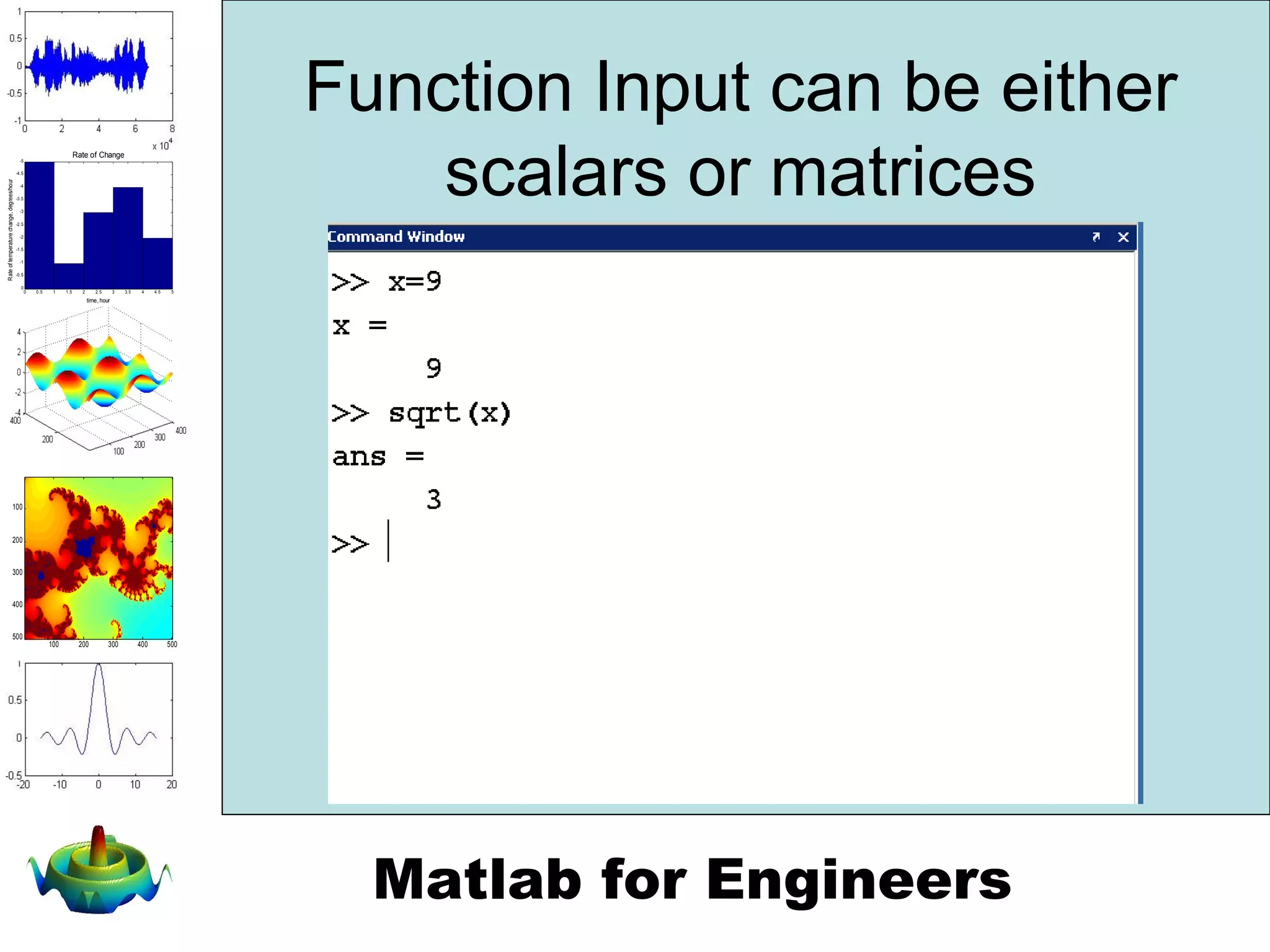
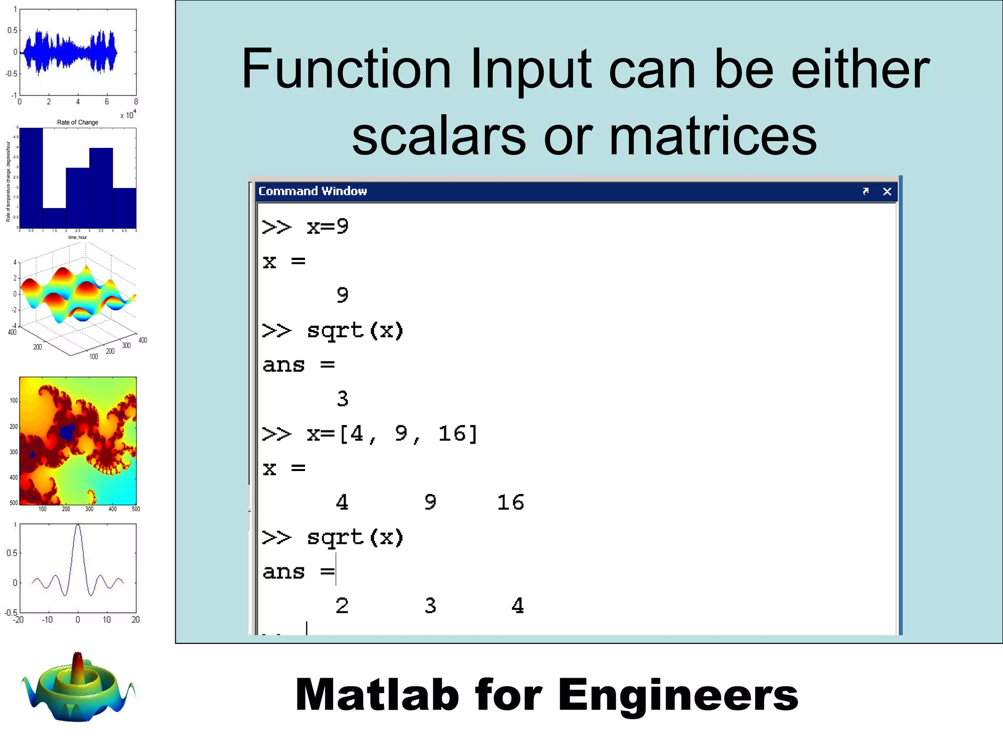
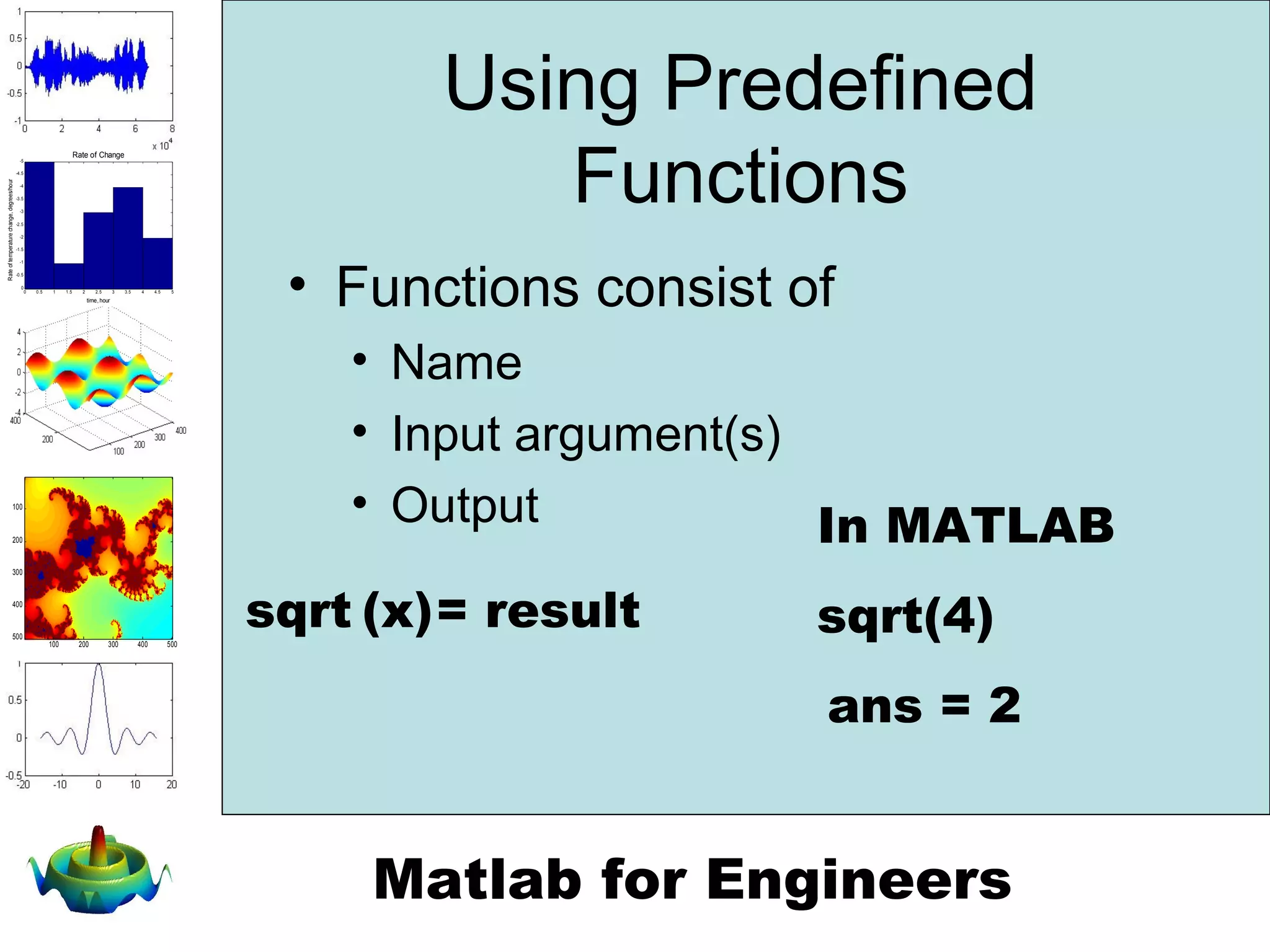
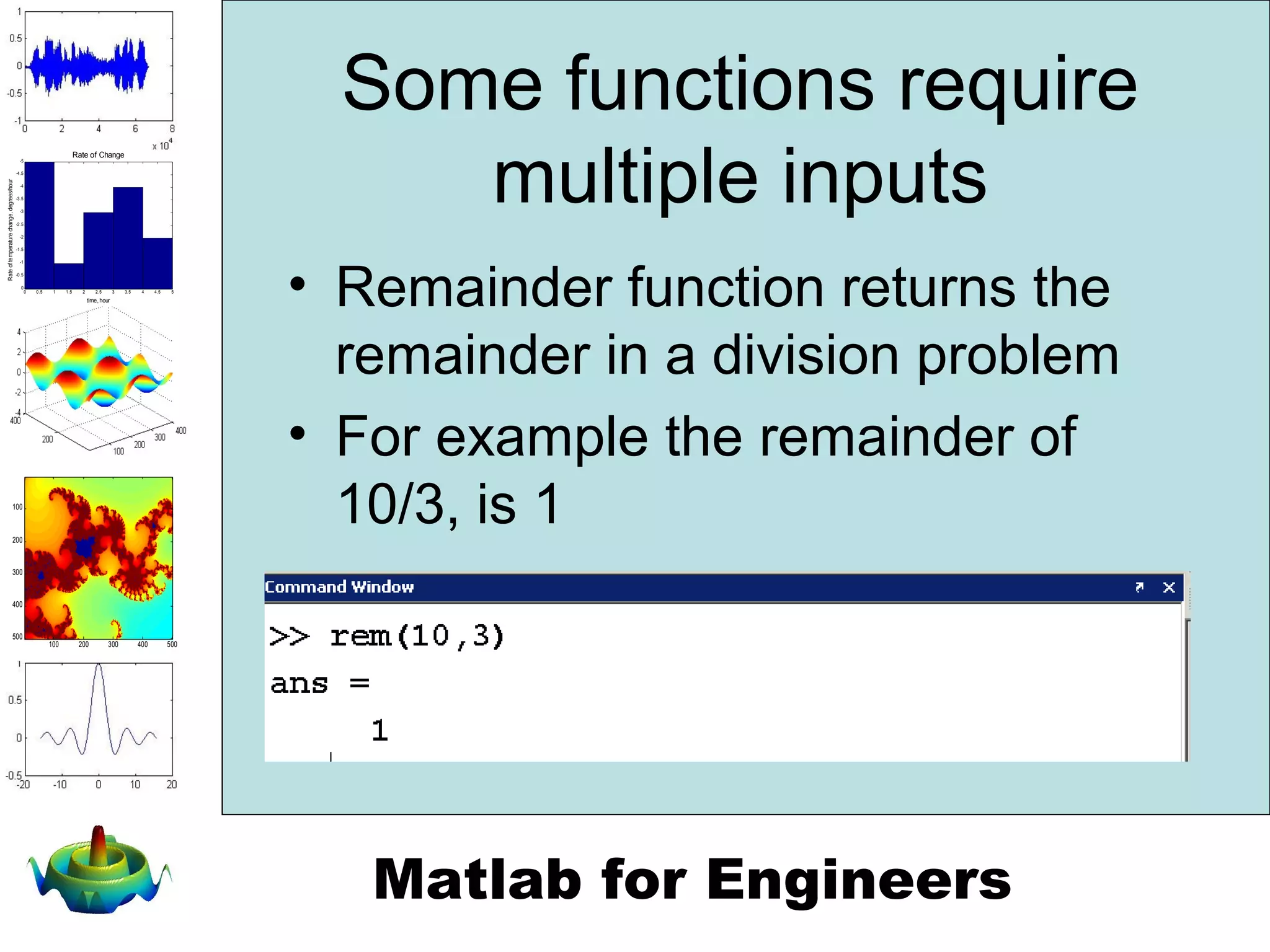
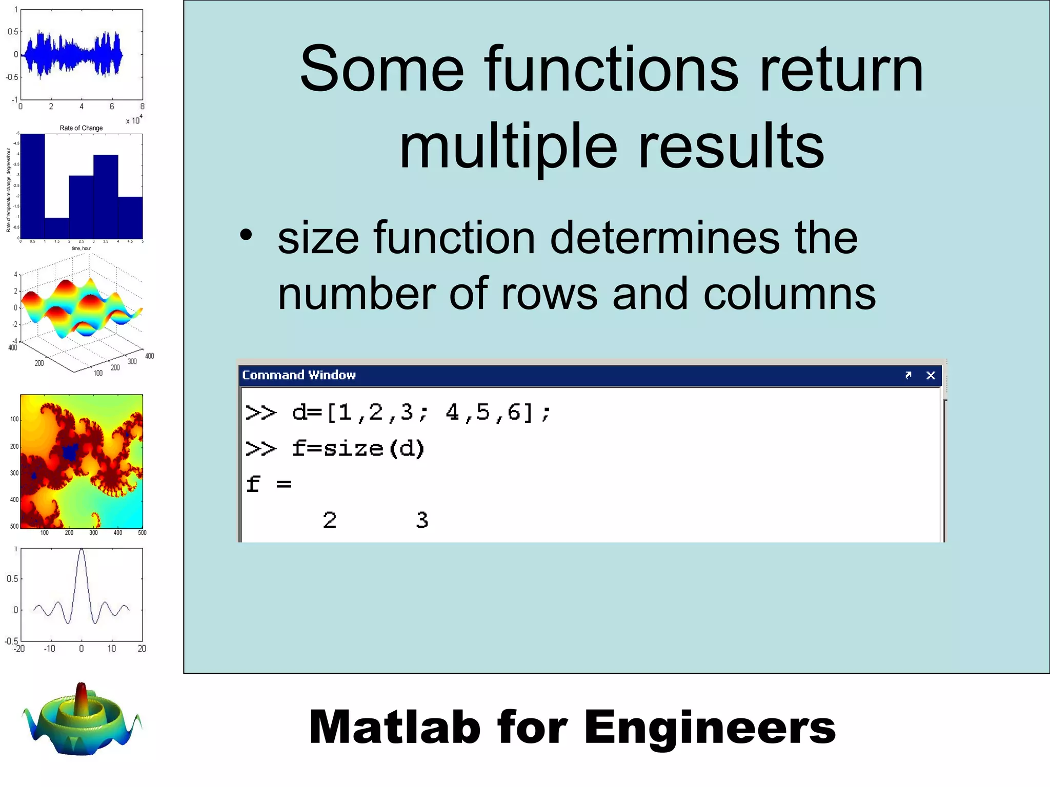
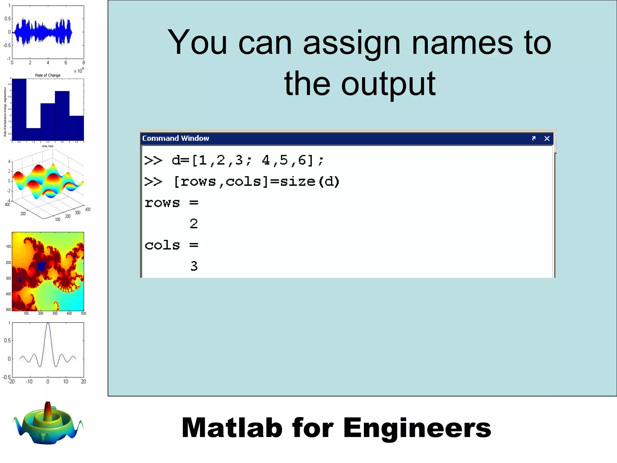
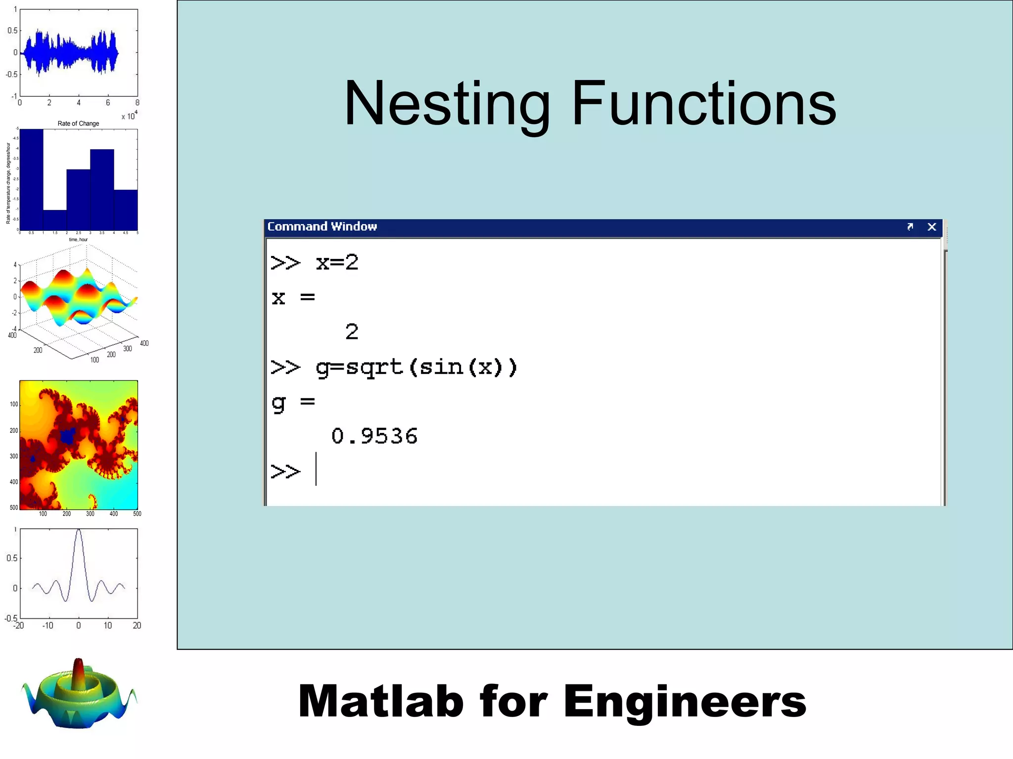
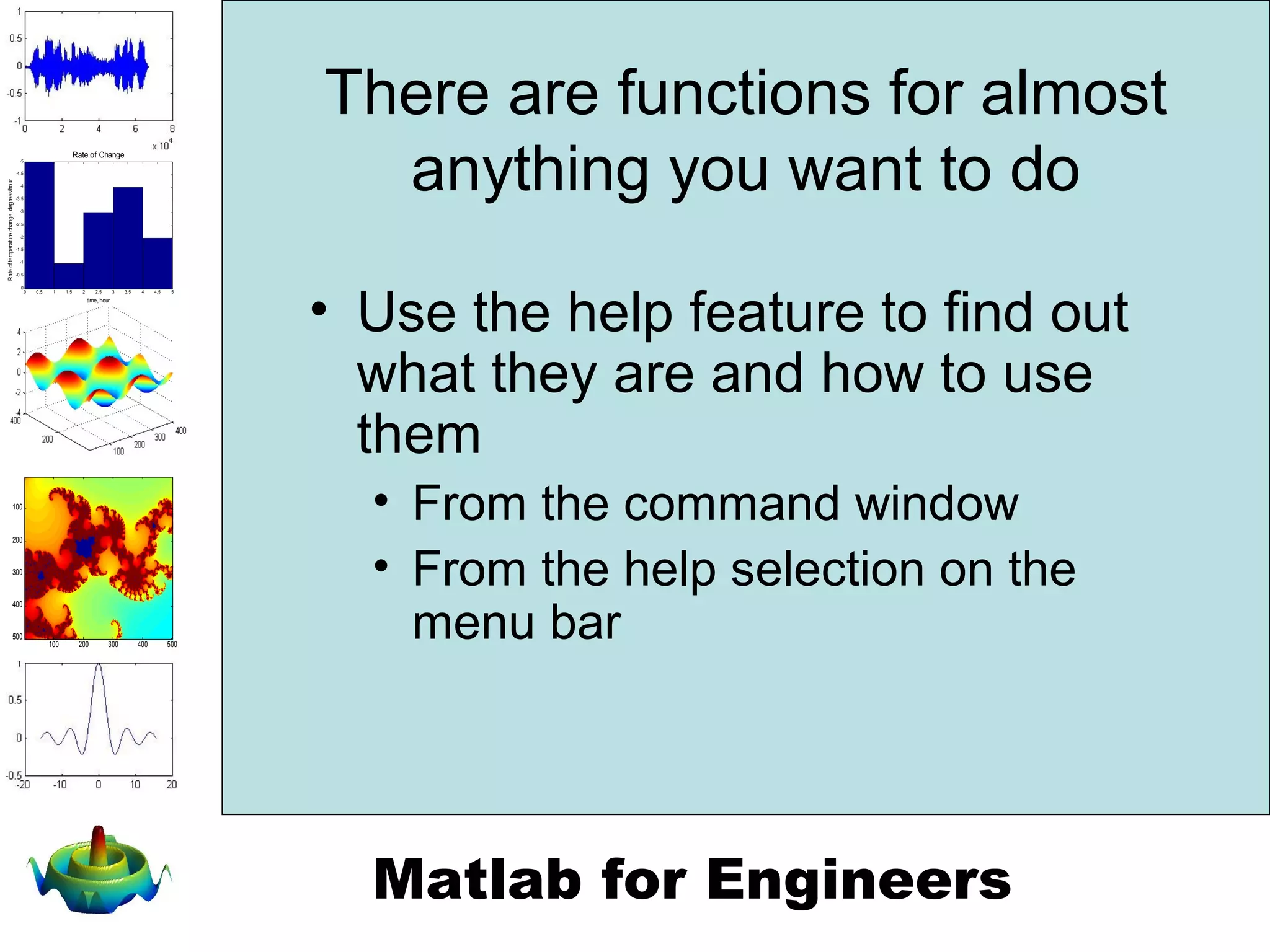
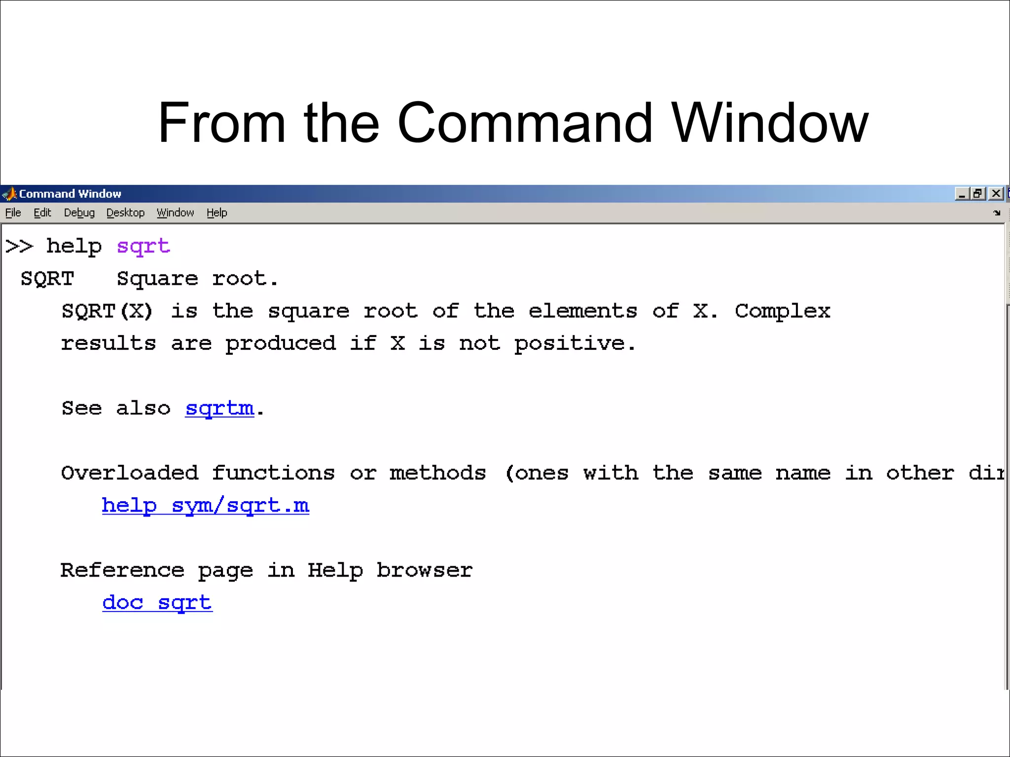
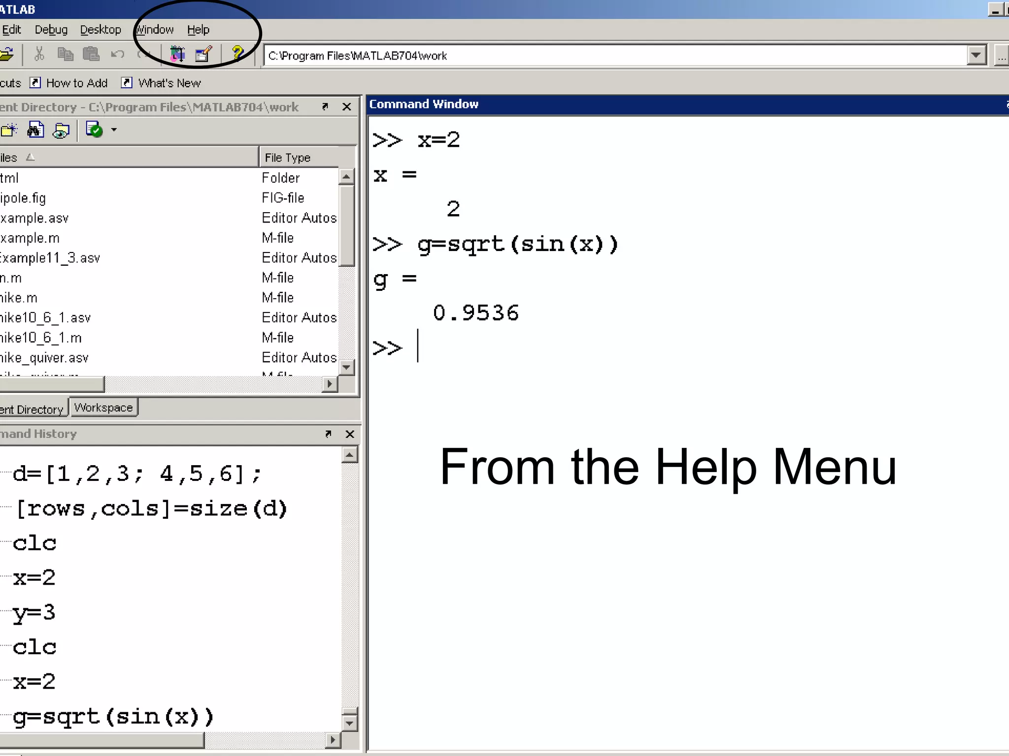
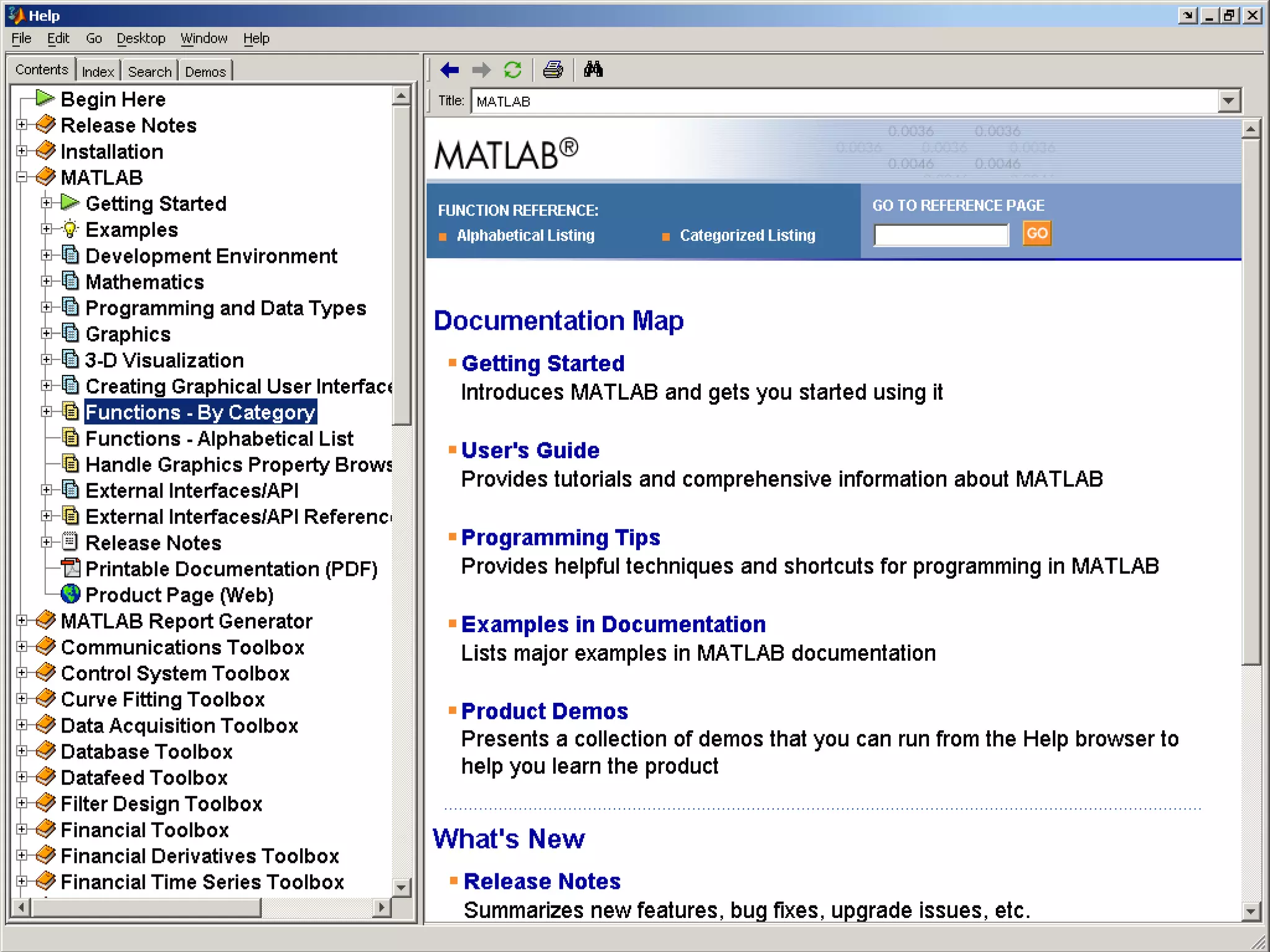
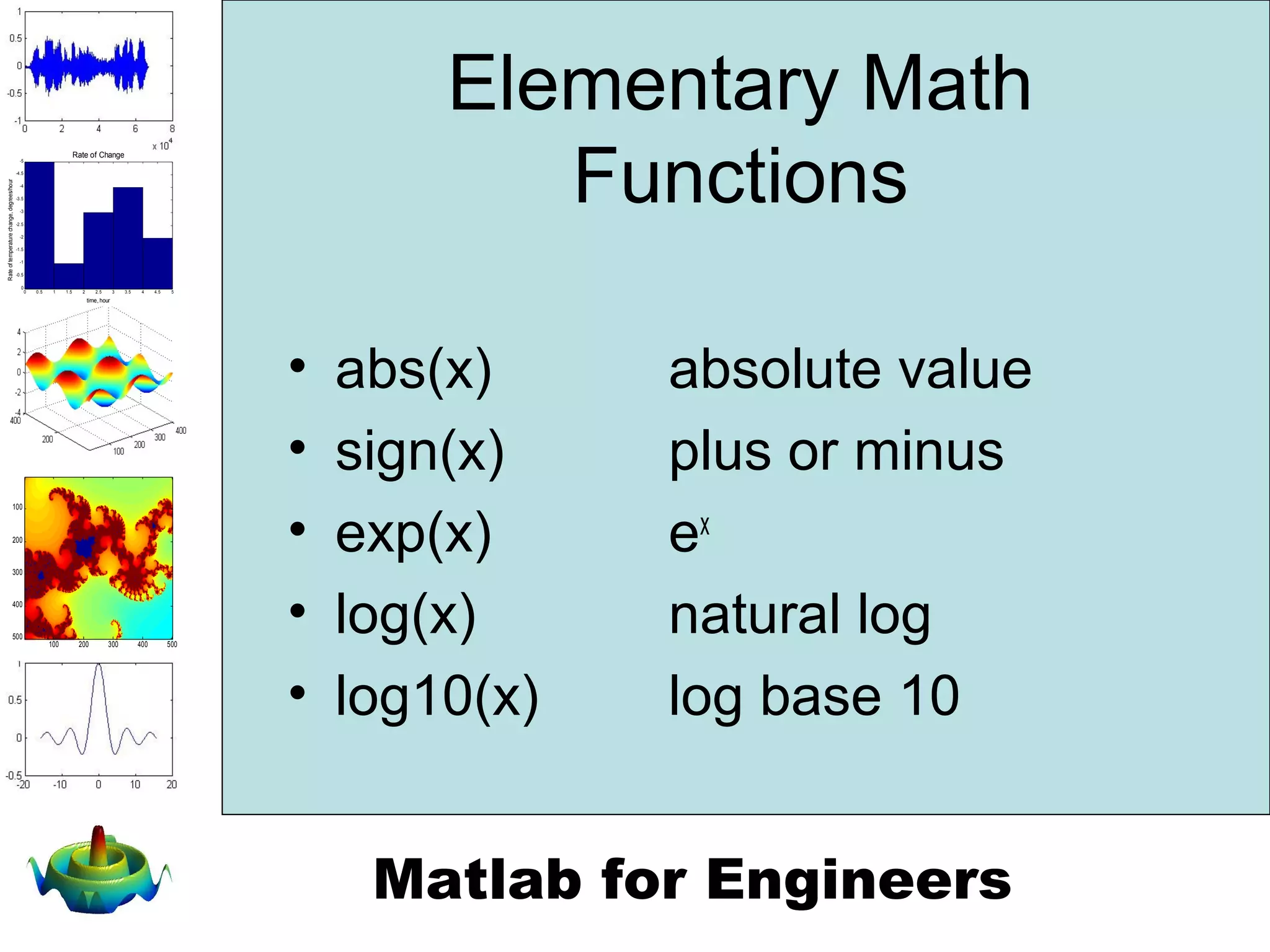
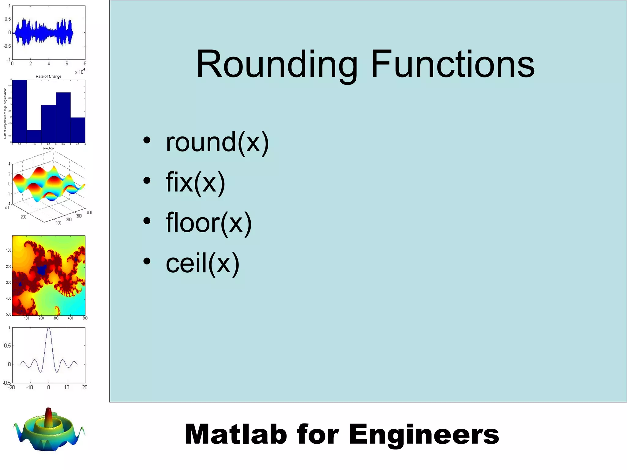
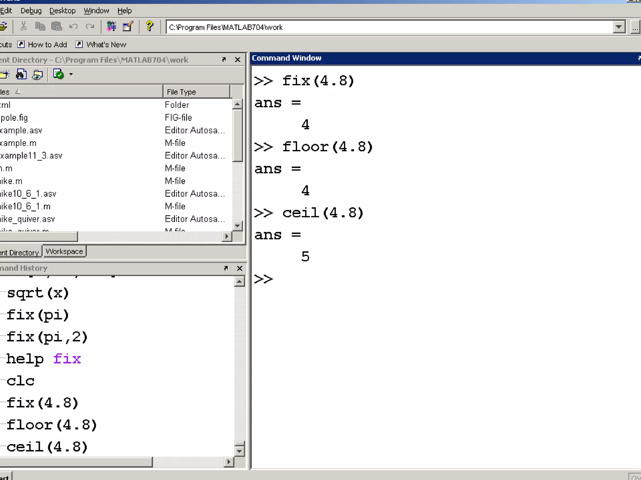
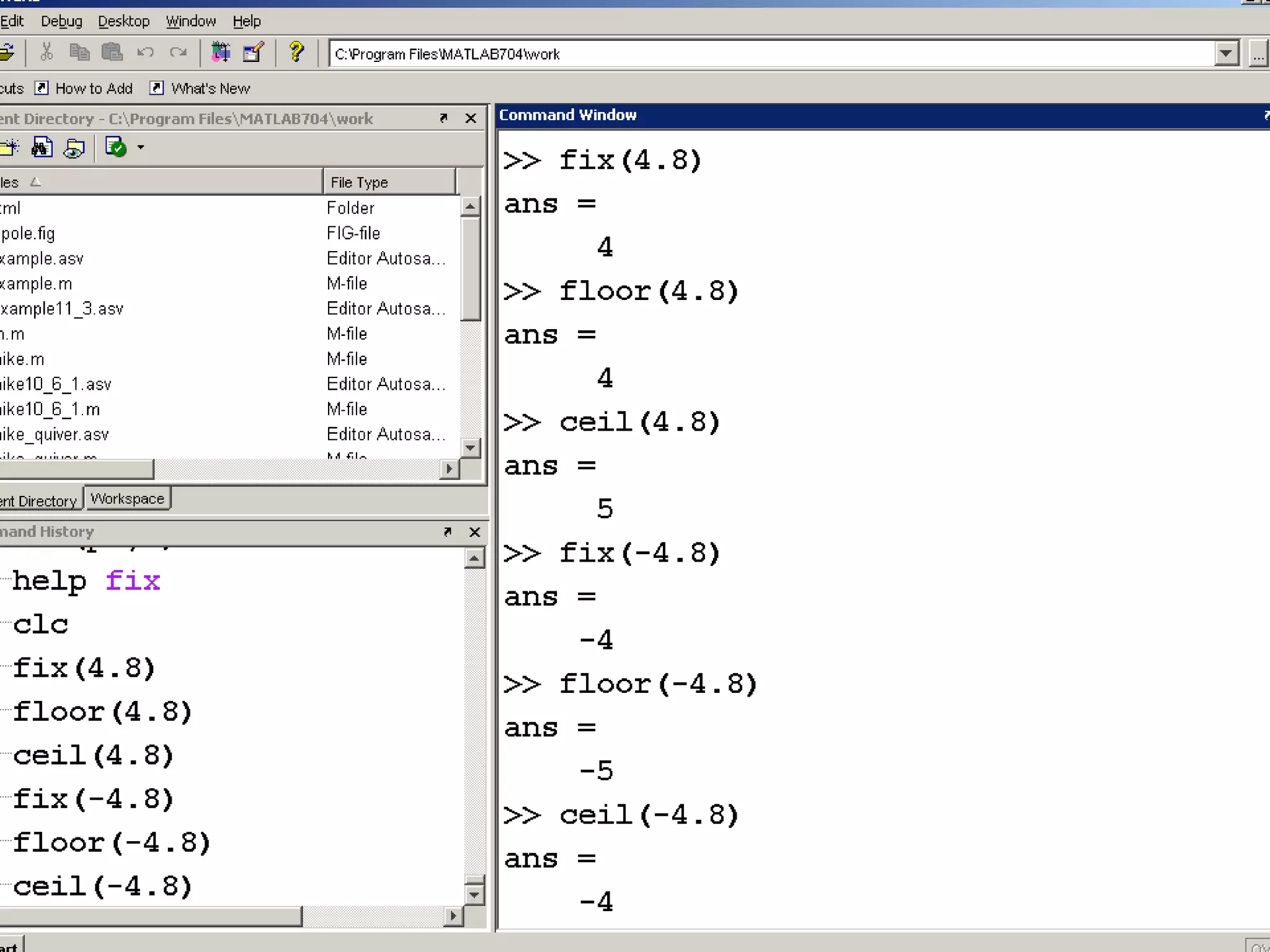
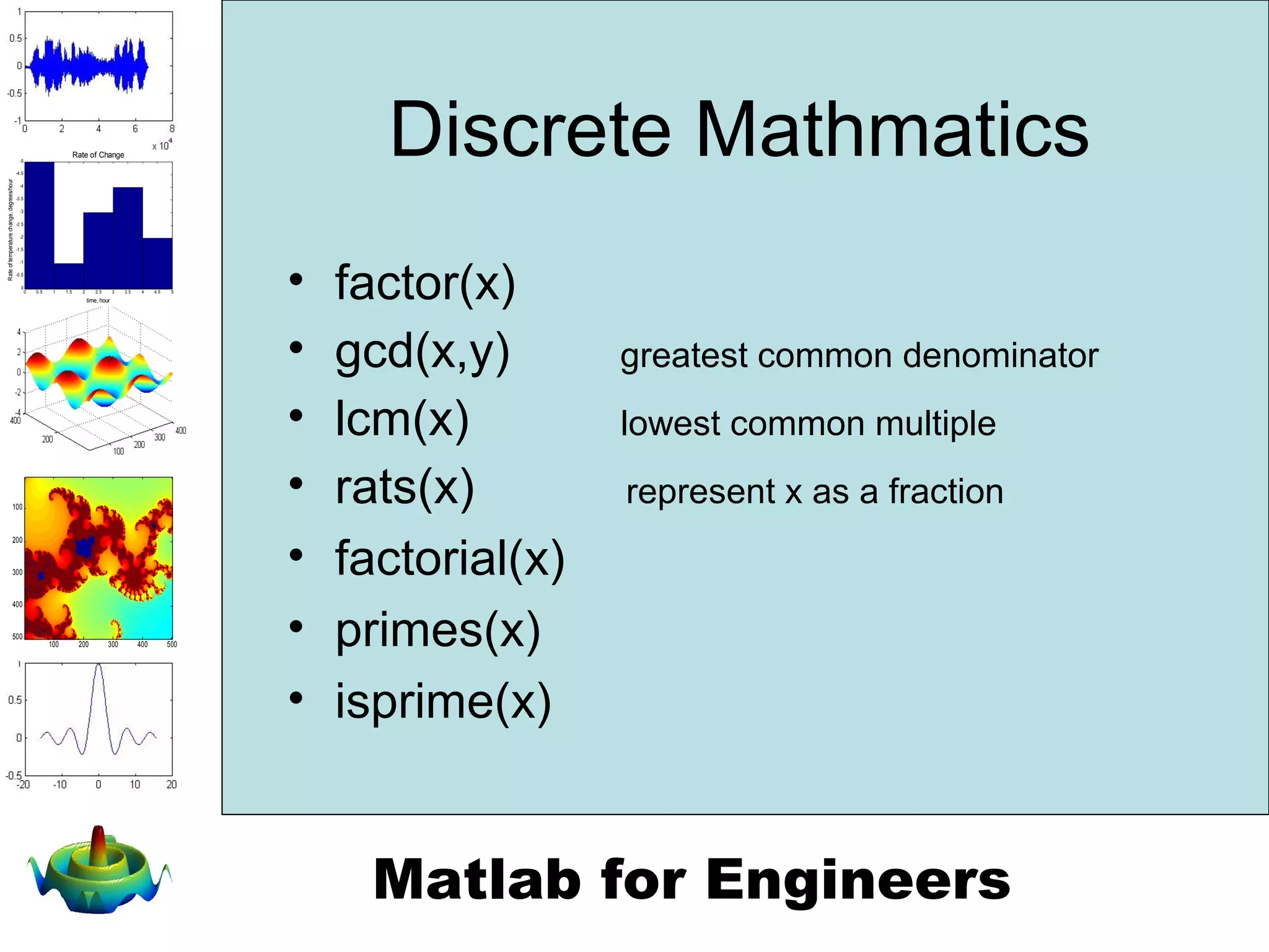
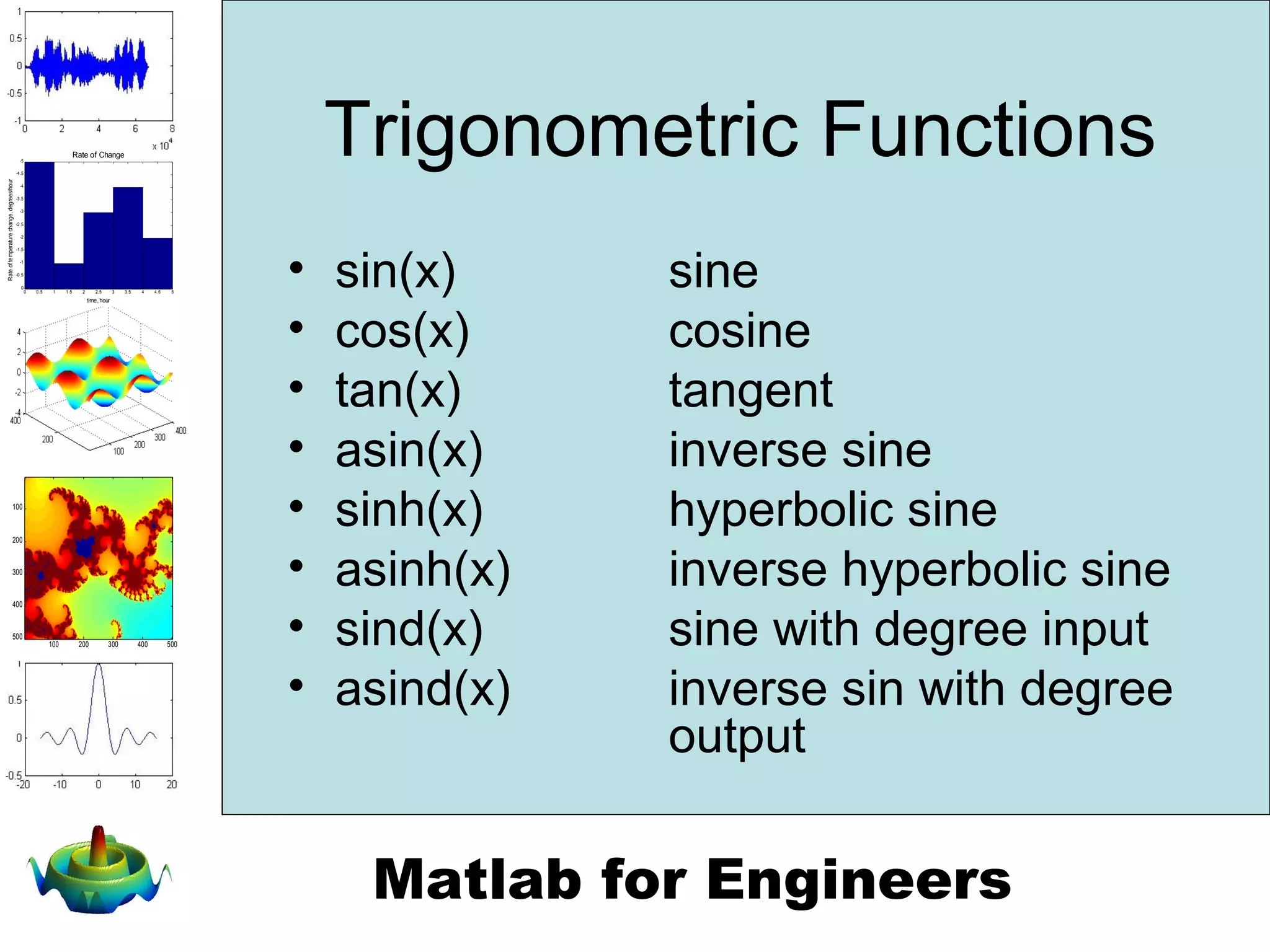
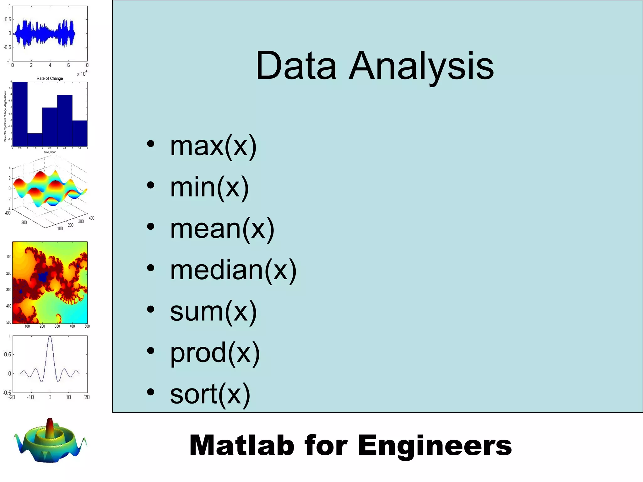
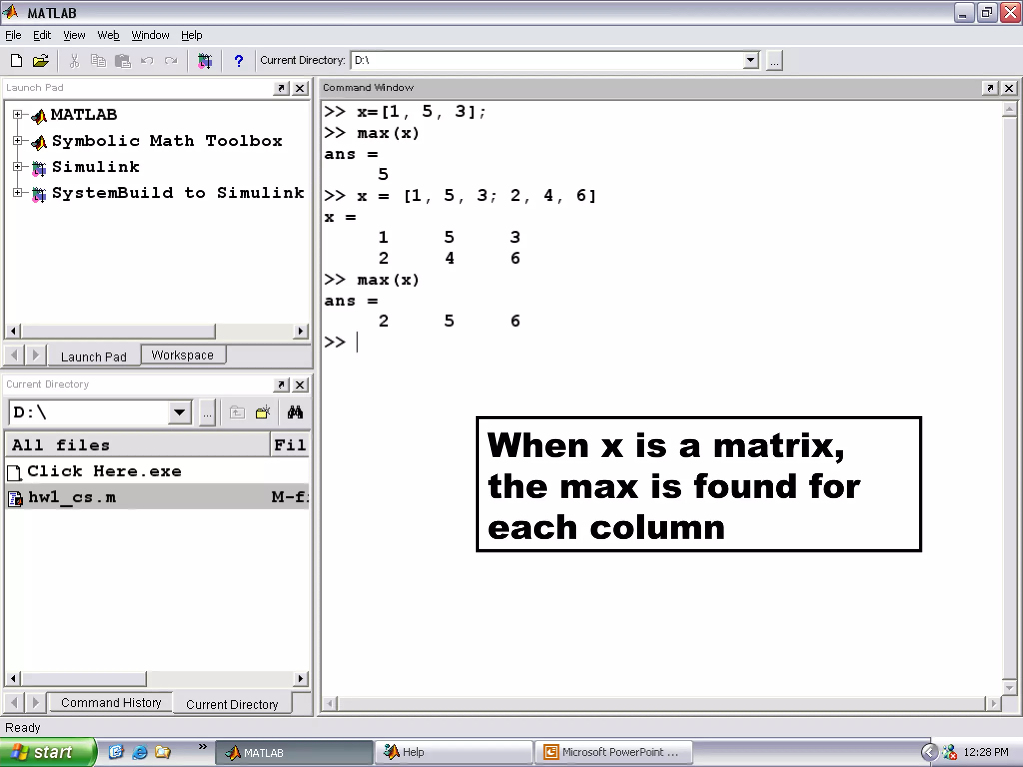
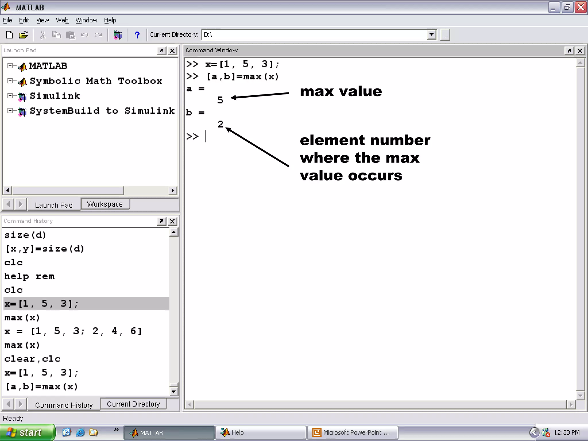
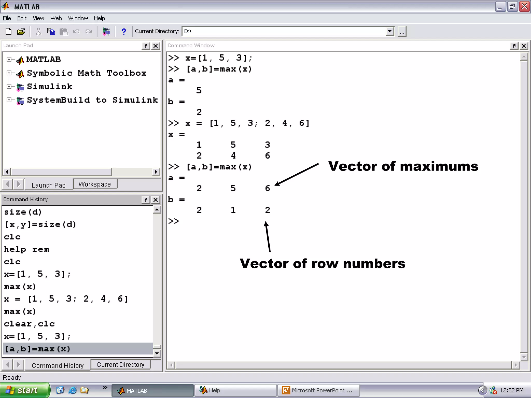
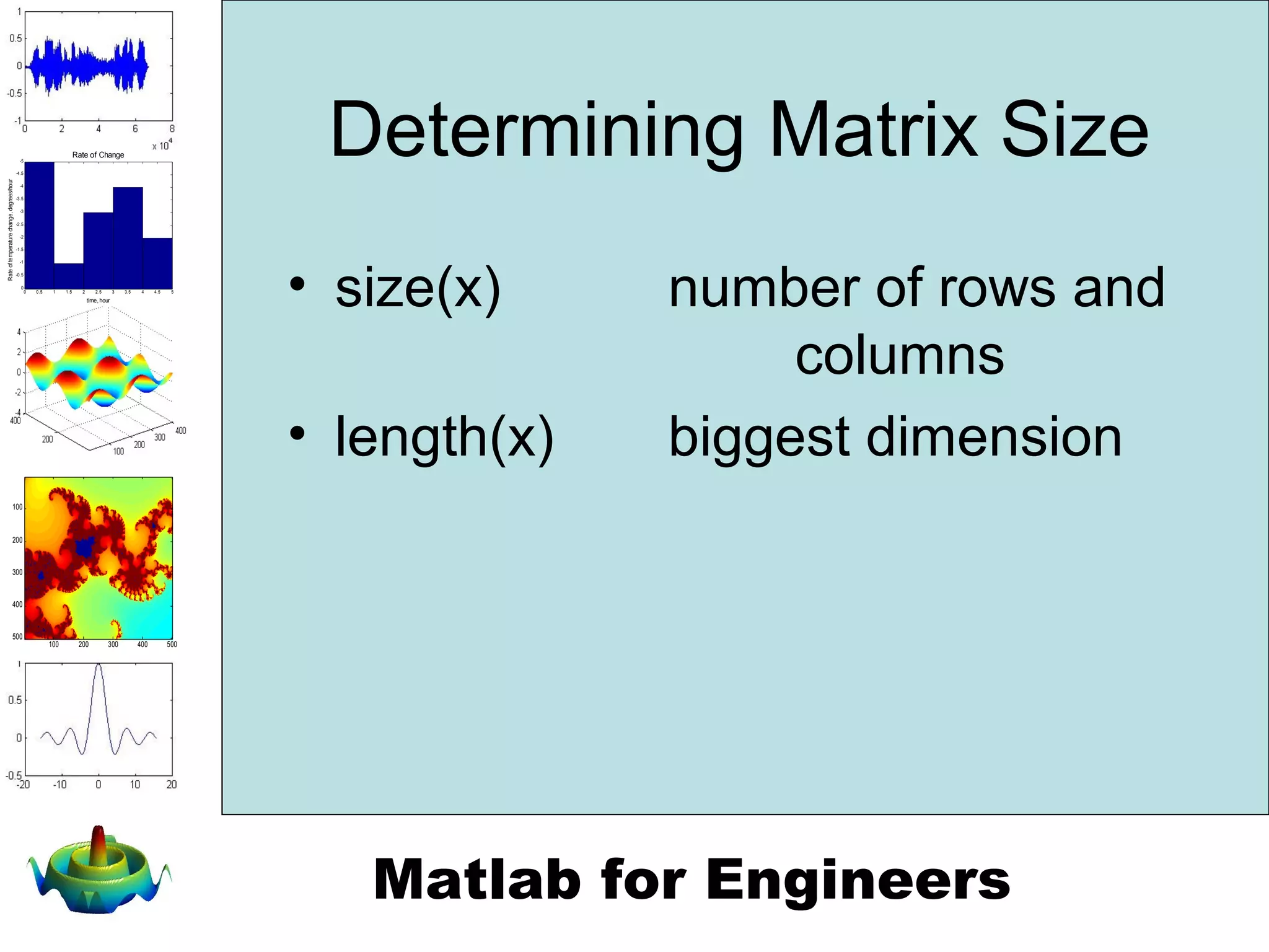
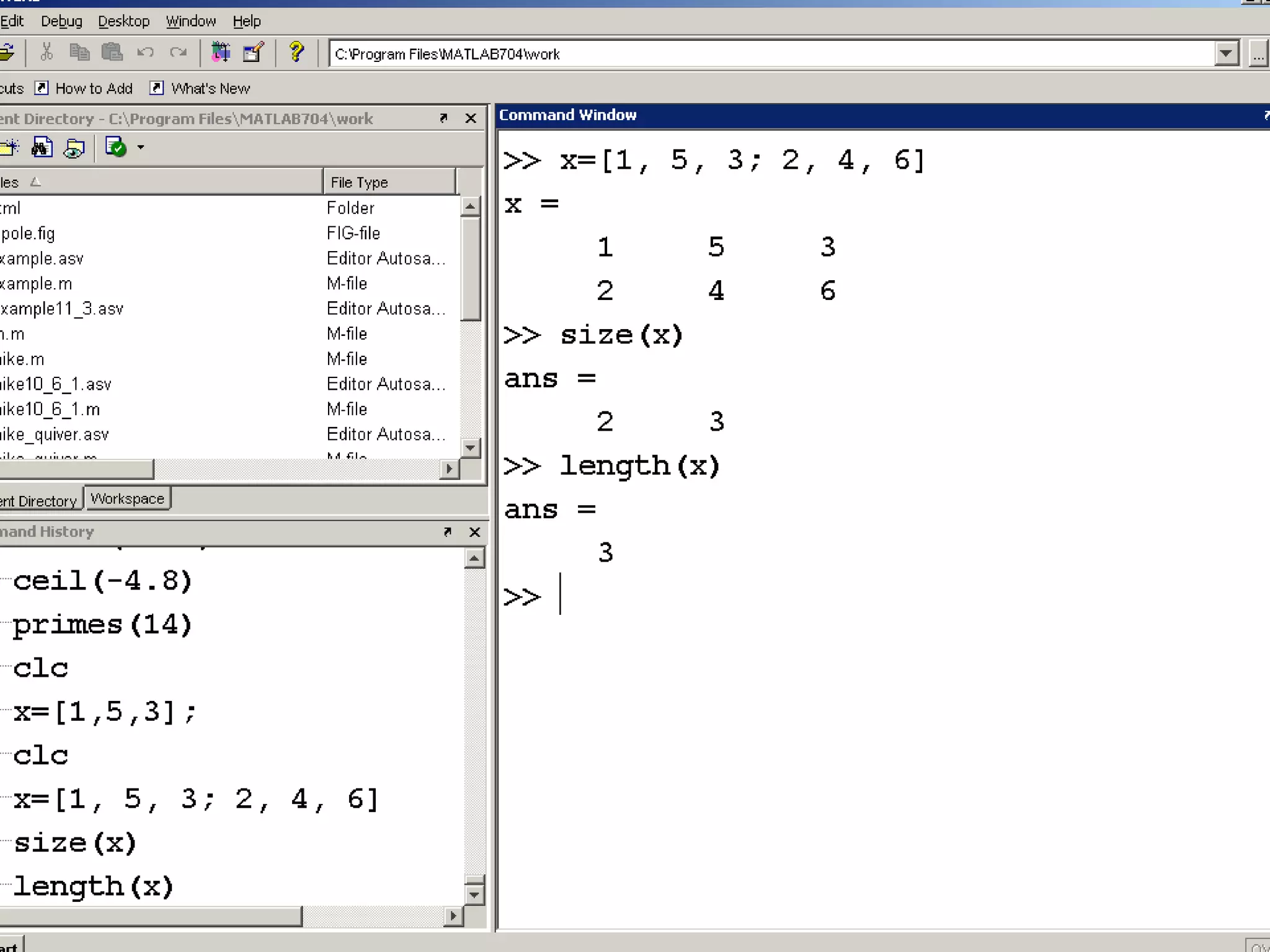
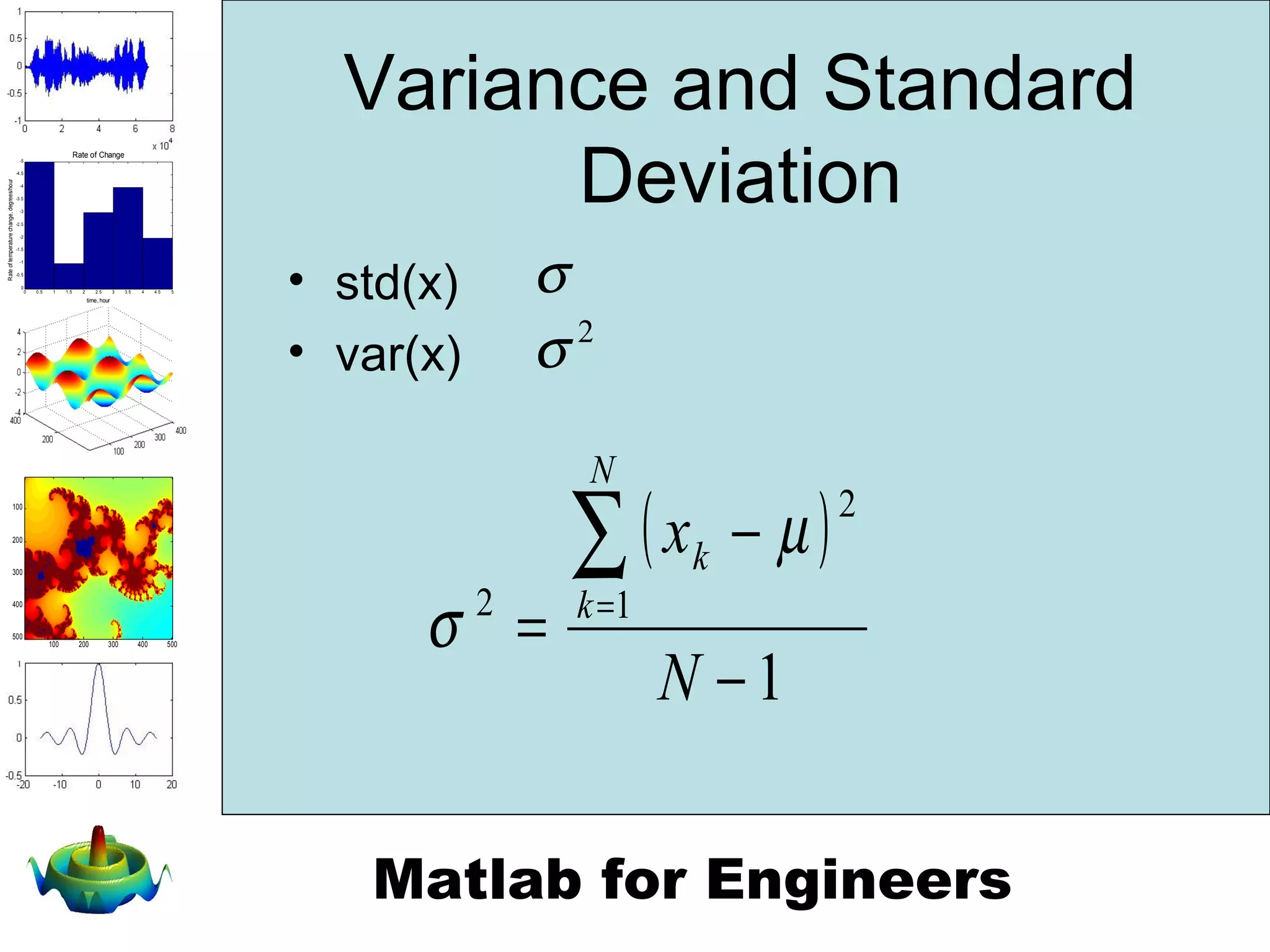
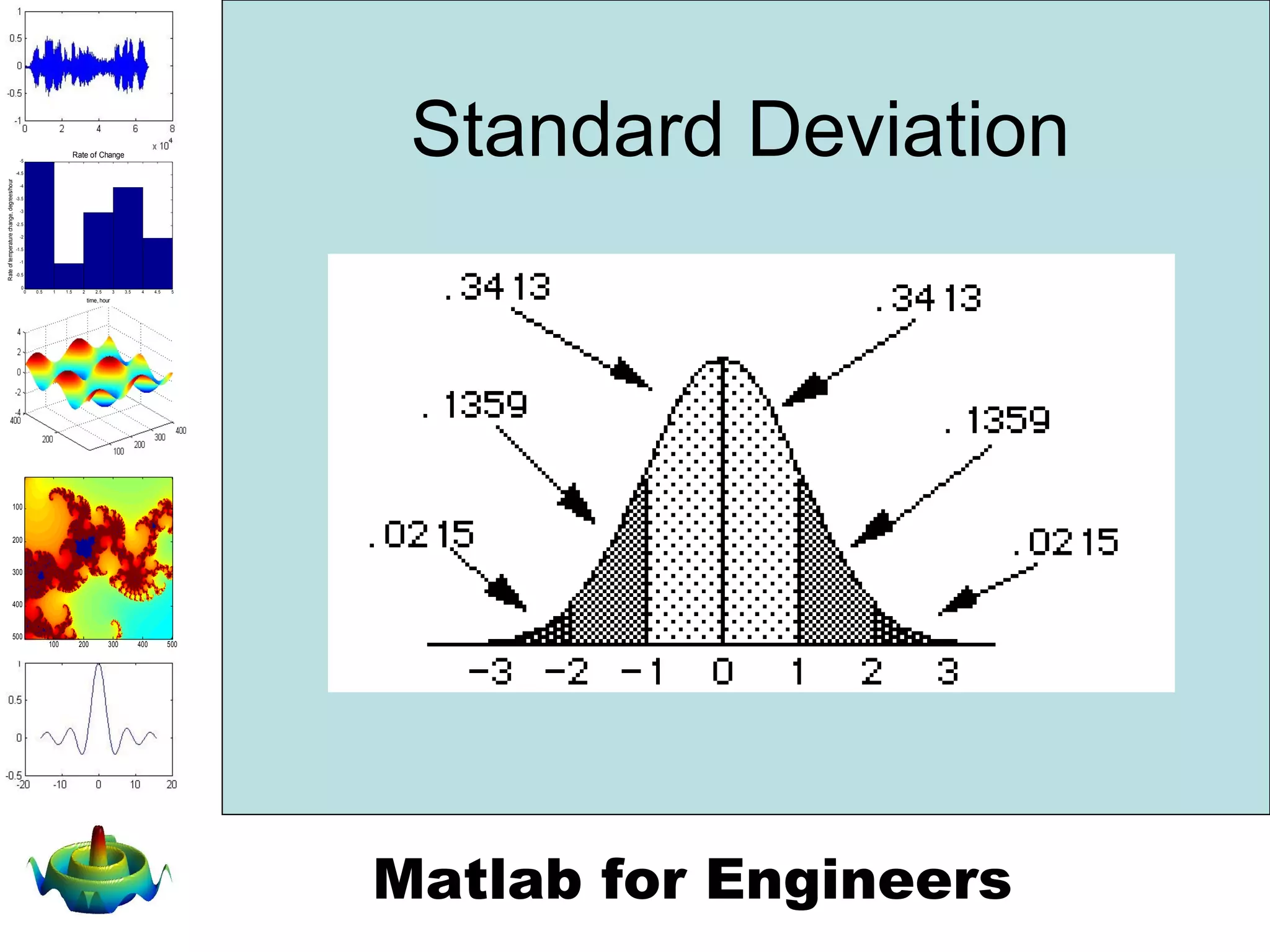
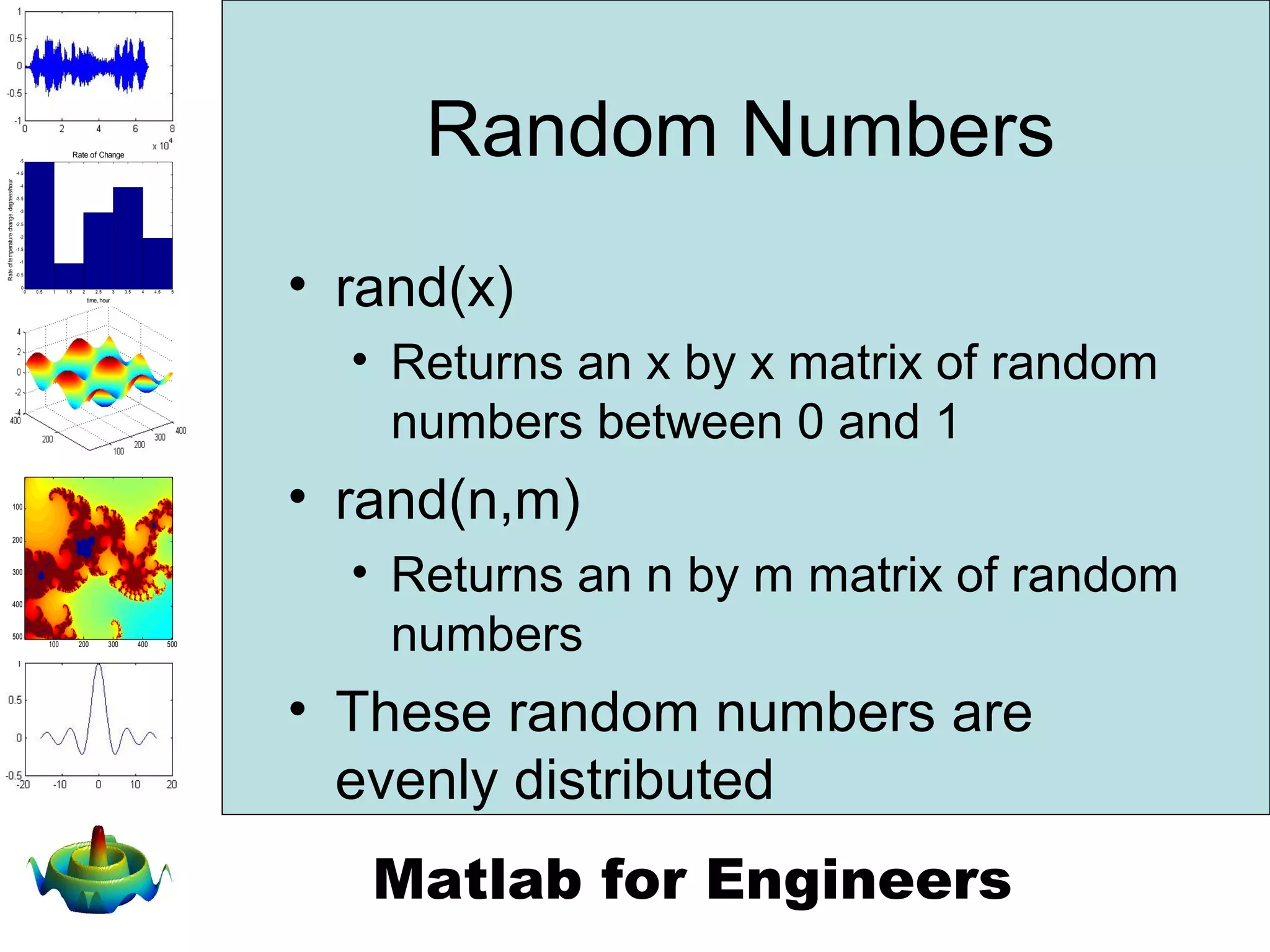
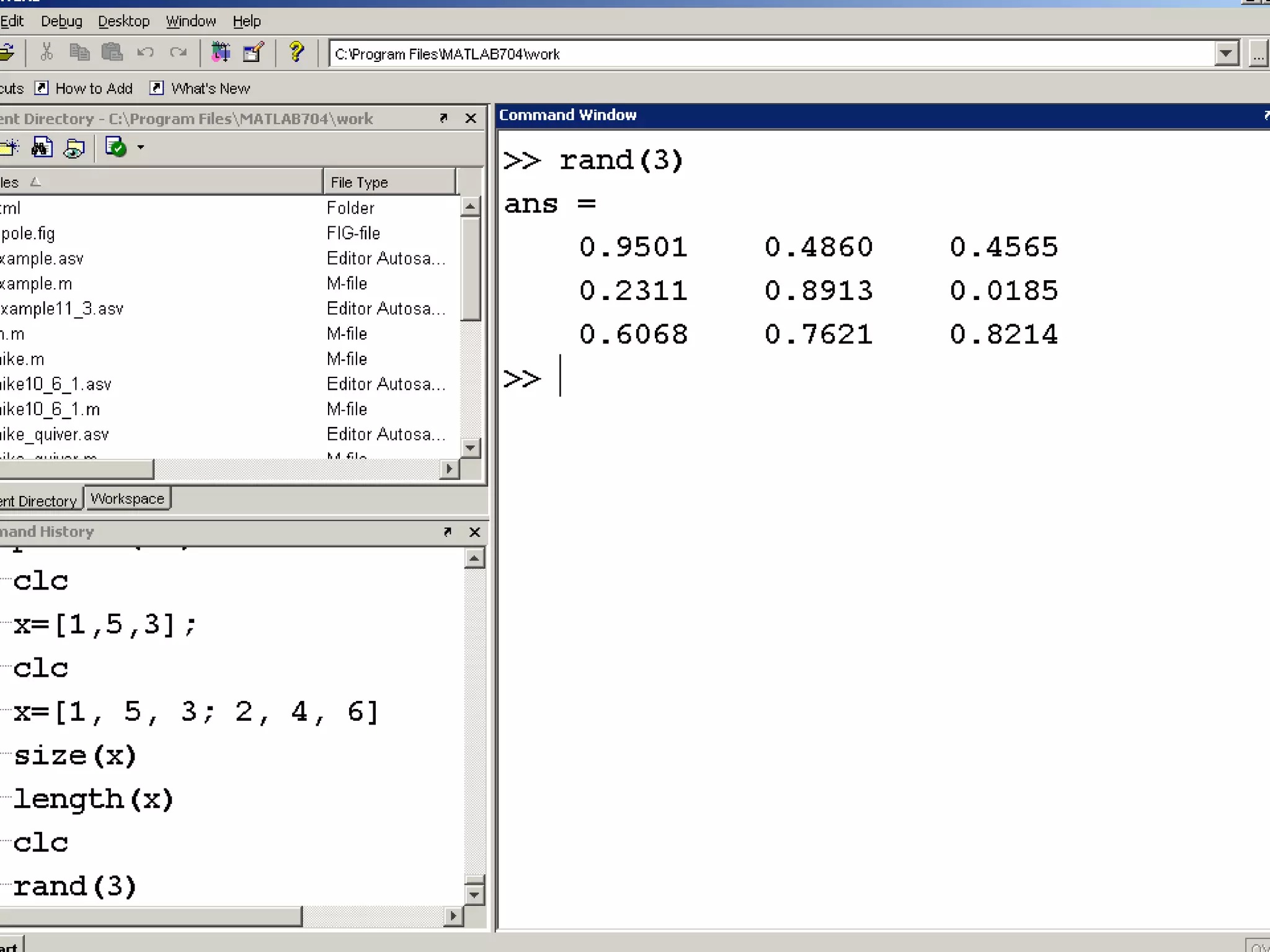
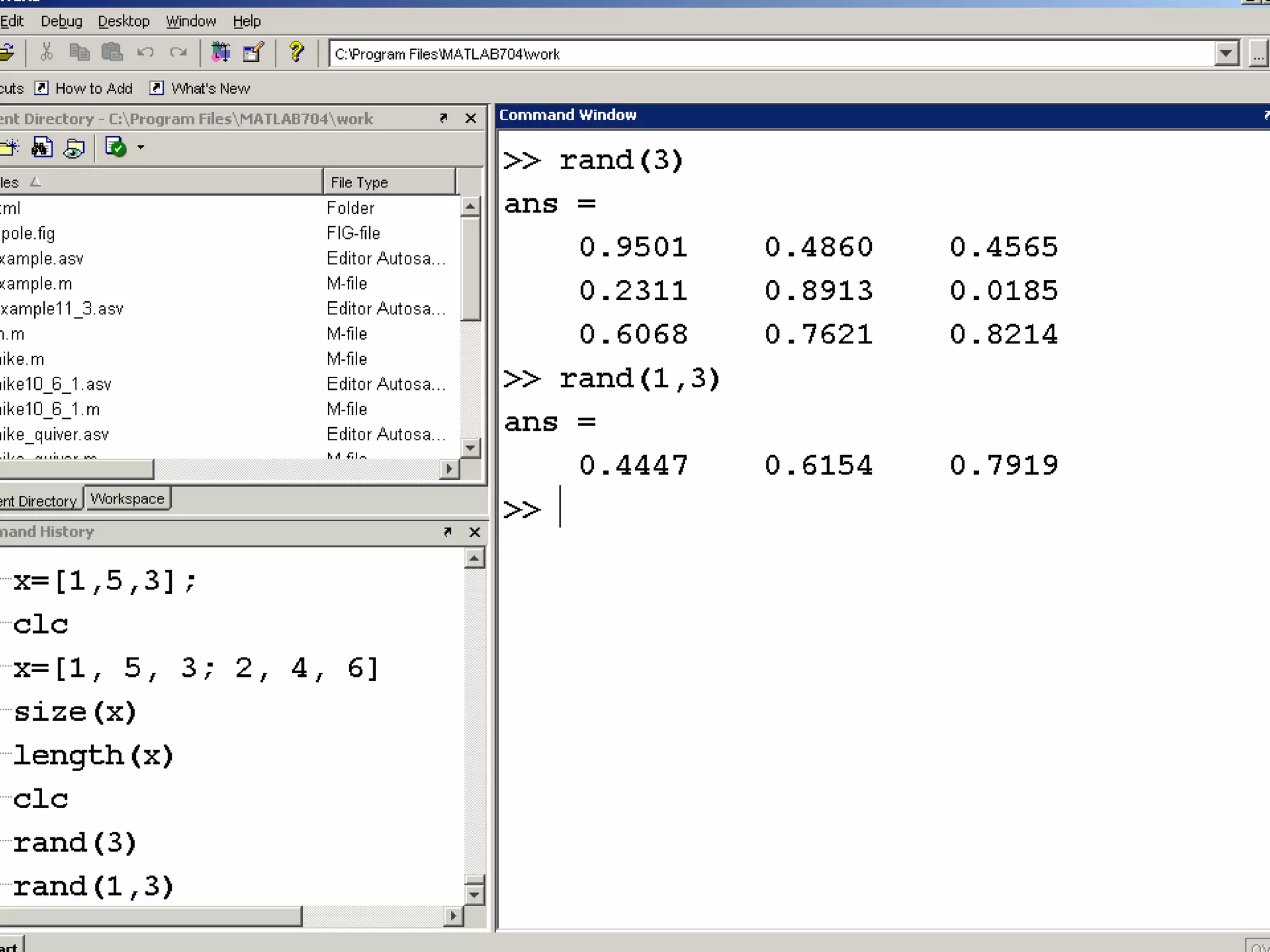
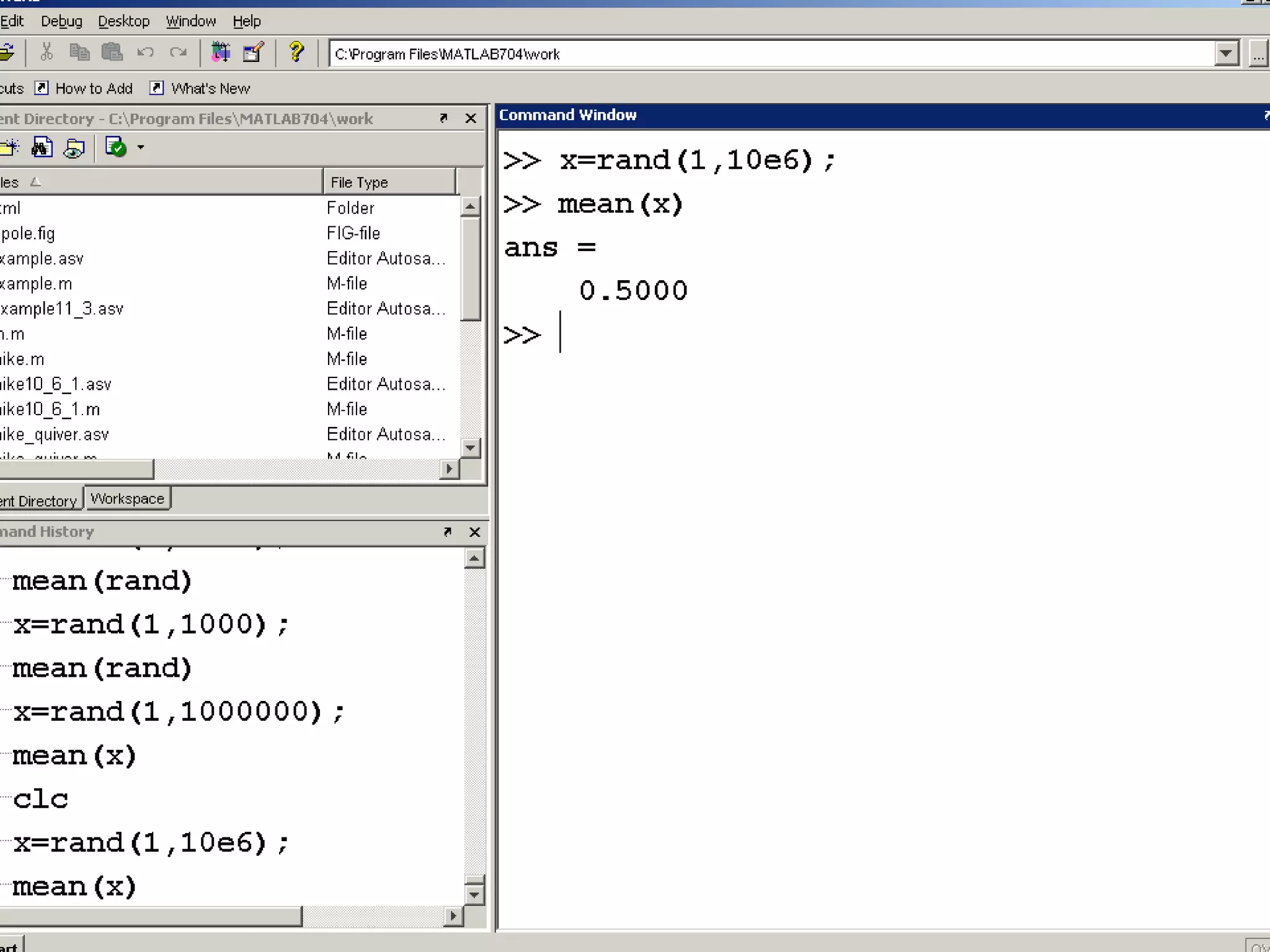
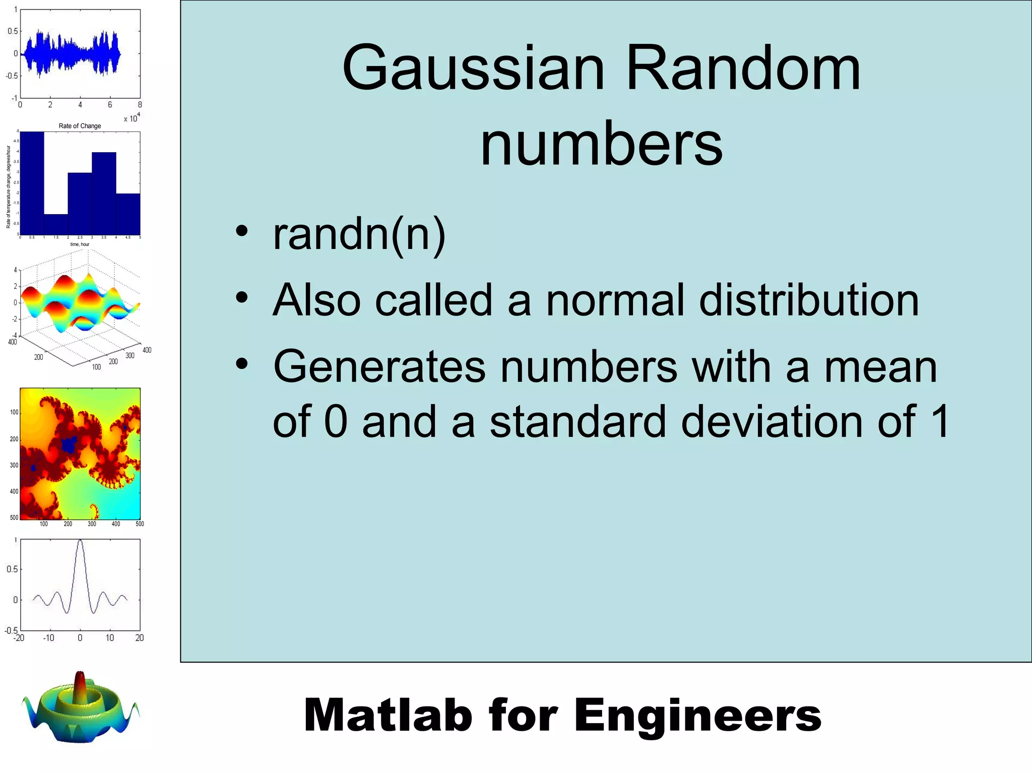
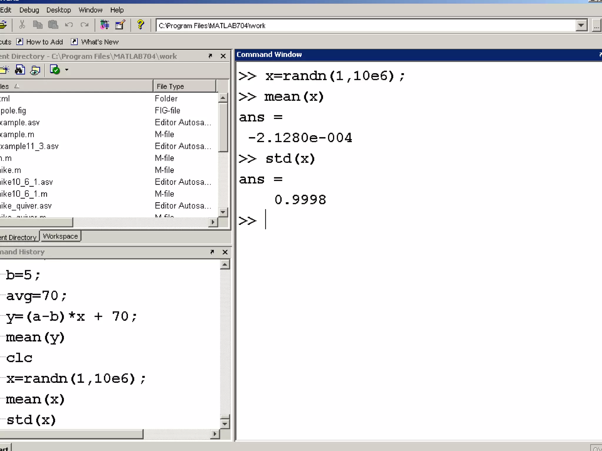
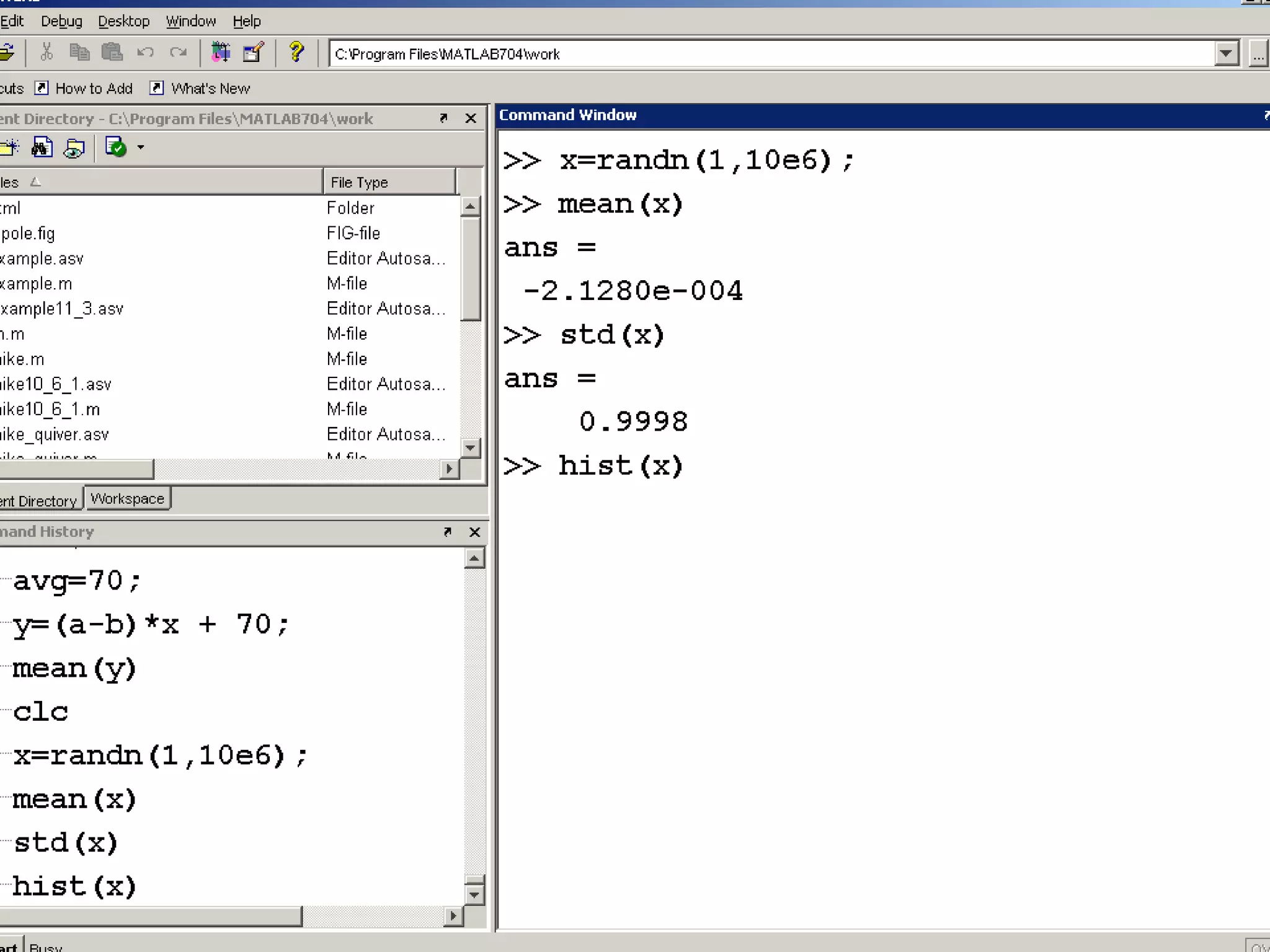
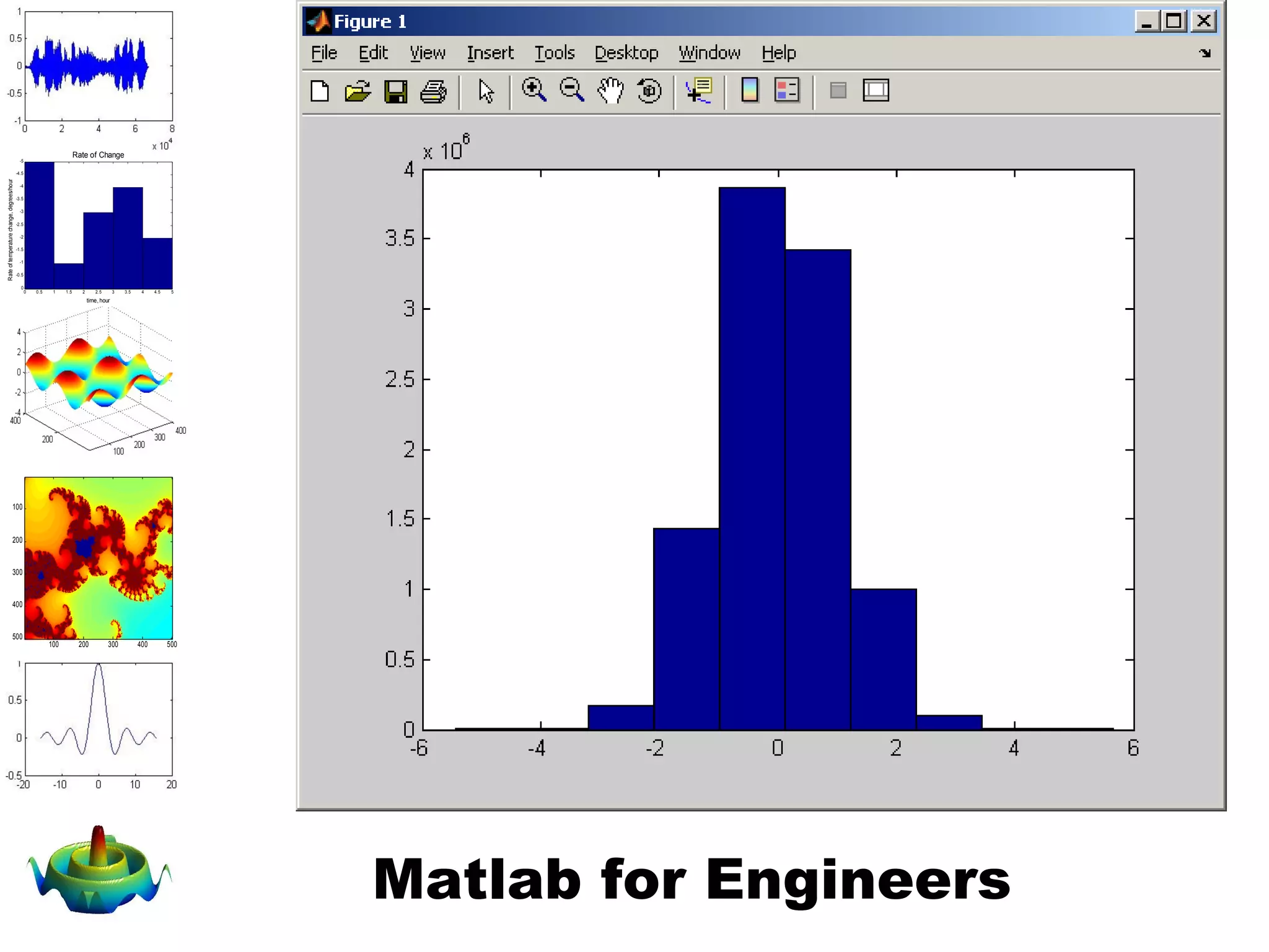
The document discusses the various built-in functions available in MATLAB for engineers. It covers fundamental math functions, trigonometric functions, data analysis functions, and how to use the help feature. Examples of functions include sqrt(), sin(), max(), and help to find documentation on any function's usage.
Matlab is basically a high level language which has many specialized toolboxes for making things easier for us.
Matlab stands for MATrix LABoratory.
The first version of MATLAB was produced in the mid 1970s as a teaching tool. MATLAB started as an interactive program for doing matrix calculations.
MATLAB has now grown to a high level mathematical language that can solve integrals and differential equations numerically and plot a wide variety of two and three Dimensional graphs.
The expanded MATLAB is now used for calculations and simulation in companies and government labs ranging from aerospace, car design, signal analysis through to instrument control and financial analysis.
In practice, it provides a very nice tool to implement numerical method.
- The desktop includes these panels:
Current Folder — Access your files.
Command Window — Enter commands at the command line, indicated by the prompt (>>).
Workspace — Explore data that you create or import from files.
- what we learn:
1- Introduction to Matlab.
2- MATLAB InstallationVersion 2018.
3- Assignment.
4- Operations in MATLAB.
5- Vectors and Matrices in MATLAB.
Introduction to Matlab
Lecture 1:
Introduction: What is Matlab, History of Matlab, strengths, weakness
Getting familiar with the interface: Layout, Pull down menus
Creating and manipulating objects: Variables (scalars, vectors, matrices, text strings), Operators (arithmetic, relational, logical) and built-in functions
Changing variable is something we come across very often in Integration. There are many
reasons for changing variables but the main reason for changing variables is to convert the
integrand into something simpler and also to transform the region into another region which is
easy to work with. When we convert into a new set of variables it is not always easy to find the
limits. So, before we move into changing variables with multiple integrals we first need to see
how the region may change with a change of variables. In order to change variables in an
integration we will need the Jacobian of the transformation.
A short presentation on the topic Numerical Integration for Civil Engineering students.
This presentation consist of small introduction about Simpson's Rule, Trapezoidal Rule, Gaussian Quadrature and some basic Civil Engineering problems based of above methods of Numerical Integration.
A basic overview, application and usage of MATLAB for engineers. It covered very basics essential that will help one to get started with MATLAB programming easily.
Provided by IDEAS2IGNITE
Here is my slide on MATLAB which includes Introduction to MATLAB, what is MATLAB, Programming languages in MATLAB, Uses of MATLAB, MATLAB features,tools and Advance tools, Advantages and disadvantages of MATLAB, Applications of MATLAB.
A Powerpoint Presentation designed to provide beginners to MATLAB an introduction to the MATLAB environment and introduce them to the fundamentals of MATLAB including matrix generation and manipulation, Arrays, MATLAB Graphics, Data Import and Export, etc
Advanced MATLAB Tutorial for Engineers & ScientistsRay Phan
This is a more advanced tutorial in the MATLAB programming environment for upper level undergraduate engineers and scientists at Ryerson University. The first half of the tutorial covers a quick review of MATLAB, which includes how to create vectors, matrices, how to plot graphs, and other useful syntax. The next part covers how to create cell arrays, logical operators, using the find command, creating Transfer Functions, finding the impulse and step response, finding roots of equations, and a few other useful tips. The last part covers more advanced concepts such as analytically calculating derivatives and integrals, polynomial regression, calculating the area under a curve, numerical solutions to differential equations, and sorting arrays.
This presentation gives the information about:electrical resistance strain gauges, covering syllabus of Unit-1, Sub: Experimental stress analysis for BE course.
MATLAB Programs For Beginners. | Abhi SharmaAbee Sharma
This is MATLAB's 10 most easy & most basic programs that I's supposed to submit in my practicals. In this document I've complied 10 MATLAB programs from basic to advanced through intermediate levels, But overall they are for beginners only. It's only a 26 pages doc. for academic purposes. well, What else a student can offer you, huh? LOLz
Assembly of screw jack, Computer Aided Machine Drawing (CAMD) of VTU Syllabus prepared by Hareesha N Gowda, Asst. Prof, Dayananda Sagar College of Engg, Blore. Please write to hareeshang@gmail.com for suggestions and criticisms.
FDM Numerical solution of Laplace Equation using MATLABAya Zaki
Finite Difference Method Numerical solution of Laplace Equation using MATLAB. 2 computational methods are used.
U can vary the number of grid points and the boundary conditions
Autonomic Resource Provisioning for Cloud-Based SoftwarePooyan Jamshidi
9th International Symposium on Software Engineering for Adaptive and Self-Managing Systems (SEAMS'14) @ ICSE 2014, for more information please refer to: http://computing.dcu.ie/~pjamshidi/PDF/SEAMS2014.pdf
Alex Smola, Professor in the Machine Learning Department, Carnegie Mellon Uni...MLconf
Fast, Cheap and Deep – Scaling Machine Learning: Distributed high throughput machine learning is both a challenge and a key enabling technology. Using a Parameter Server template we are able to distribute algorithms efficiently over multiple GPUs and in the cloud. This allows us to design very fast recommender systems, factorization machines, classifiers, and deep networks. This degree of scalability allows us to tackle computationally expensive problems efficiently, yielding excellent results e.g. in visual question answering.
In this Dagstuhl talk, I presented my current research on cloud auto-scaling and component connector self-adaptation and how I employed type-2 fuzzy control to tame the uncertainty regarding knowledge specification.
Monitoring Complex Systems: Keeping Your Head on Straight in a Hard WorldBrian Troutwine
This talk will provide motivation for the extensive instrumentation of complex computer systems and make the argument that such systems. This talk will provide practical starting points in Erlang projects and maintain a perspective on the human organization around the computer system. Brian will focus on getting started with instrumentation in a systematic way and follow up with the challenge of interpreting and acting on metrics emitted from a production system in a way which does not overwhelm operators’ ability to effectively control or prioritize faults in the system. He’ll use historical examples and case studies from my work to keep the talk anchored in the practical.
Talk objectives:
Brian hopes to convince the audience of two things:
* that monitoring and instrumentation is an essential component of any long-lived system and
* that it's not so hard to get started, after all.
He’ll keep a clear-eyed view of what works and is difficult in practice so that the audience can make a reasoned decision after the talk.
Target audience:
This talk would appeal to engineers with long-running production employments, operations folks and Erlangers in general.
A Framework for Robust Control of Uncertainty in Self-Adaptive Software Conn...Pooyan Jamshidi
We enable reliable and dependable self‐adaptations of component connectors in unreliable environments with imperfect monitoring facilities and conflicting user opinions about adaptation policies by developing a framework which comprises: (a) mechanisms for robust model evolution, (b) a method for adaptation reasoning, and (c) tool support that allows an end‐to‐end application of the developed techniques in real‐world domains.
Marios Michailidis & Mathias Muller, H2O.ai - Time Series with H2O Driverless...Sri Ambati
This session was recorded in San Francisco on February 5th, 2019 and can be viewed here: https://youtu.be/0pvvDHfxdZ8
Driverless AI is H2O.ai's latest flagship product for automatic machine learning. It fully automates some of the most challenging and productive tasks in applied data science such as feature engineering, model tuning, model ensembling and model deployment. Driverless AI turns Kaggle-winning grandmaster recipes into production-ready code, and is specifically designed to avoid common mistakes such as under- or overfitting, data leakage or improper model validation, some of the hardest challenges in data science. Avoiding these pitfalls alone can save weeks or more for each model, and is necessary to achieve high modeling accuracy.
Driverless AI is now equipped with time-series functionality. Time series helps forecast sales, predict industrial machine failure and more. With the time series capability in Driverless AI, H2O.ai directly addresses some of the most pressing concerns of organizations across industries for use cases such as transactional data in capital markets, in retail to track in-store and online sales, and in manufacturing with sensor data to improve supply chain or predictive maintenance.
Bio: Marios Michailidis is a Competitive Data Scientist at H2O.ai. He holds a Bsc in accounting Finance from the University of Macedonia in Greece, an Msc in Risk Management from the University of Southampton and a PhD in machine learning at from UCL . He has worked in both marketing and credit sectors in the UK Market and has led many analytics’ projects with various themes including: acquisition, retention, recommenders, fraud detection, portfolio optimization and more. He is the creator of KazAnova, a freeware GUI for credit scoring and data mining 100% made in Java as well as is the creator of StackNet Meta-Modelling Framework. In his spare time he loves competing on data science challenges and was ranked 1st out of 500,000 members in the popular Kaggle.com data competition platform. He currently ranks 3rd.
Bio: A Kaggle Grandmaster and a Data Scientist at H2O.ai, Mathias Müller holds an AI and ML focused diploma (eq. M.Sc.) in computer science from Humboldt University in Berlin. During his studies, he keenly worked on computer vision in the context of bio-inspired visual navigation of autonomous flying quadrocopters. Prior to H2O.ai, he as a machine learning engineer for FSD Fahrzeugsystemdaten GmbH in the automotive sector. His stint with Kaggle was a chance encounter as he stumbled upon the data competition platform while looking for a more ML-focused platform as compared to TopCoder. This is where he entered his first predictive modeling competition and climbed up the ladder to be a Grandmaster. He is an active contributor to XGBoost and is working on Driverless AI with H2O.ai.
Similar to Chapter 3 -Built-in Matlab Functions (20)
Marios Michailidis & Mathias Muller, H2O.ai - Time Series with H2O Driverless...
Chapter 3 -Built-in Matlab Functions
1. Matlab for Engineers
100 200 300 400 500
100
200
300
400
500
0 0.5 1 1.5 2 2.5 3 3.5 4 4.5 5
-5
-4.5
-4
-3.5
-3
-2.5
-2
-1.5
-1
-0.5
0
Rate of Change
time, hour
Rateoftemperaturechange,degrees/hour
Built-in Matlab
Functions
Chapter 3 0 200 400 600 800 1000
0
20
40
60
80
100
Test Scores
Student Number
Score
0 20 40 60 80 100
0
20
40
60
80
100
120
Distribution of Test Scores
Score
#ofstudents
0 200 400 600 800 1000
0
20
40
60
80
100
Student Number
Score
0 20 40 60 80 100
0
20
40
60
80
100
120
Score
#ofstudents
Average = 50
Average = 50
Average = 50
Average = 50
2. Matlab for Engineers
100 200 300 400 500
100
200
300
400
500
0 0.5 1 1.5 2 2.5 3 3.5 4 4.5 5
-5
-4.5
-4
-3.5
-3
-2.5
-2
-1.5
-1
-0.5
0
Rate of Change
time, hour
Rateoftemperaturechange,degrees/hour
In this chapter we’ll cover
• Using Built in Functions
• Using the Help Feature
• Elementary Math Functions
• Trigonometric Functions
• Data Analysis Functions
• Random Number Functions
• Complex Number Functions
• Computational Limits
• Special Values and Miscellaneous Functions
3. Matlab for Engineers
100 200 300 400 500
100
200
300
400
500
0 0.5 1 1.5 2 2.5 3 3.5 4 4.5 5
-5
-4.5
-4
-3.5
-3
-2.5
-2
-1.5
-1
-0.5
0
Rate of Change
time, hour
Rateoftemperaturechange,degrees/hour
Matlab uses function names consistent
with most major programming languages
For example
• sqrt
• sin
• cos
• log
4. Matlab for Engineers
100 200 300 400 500
100
200
300
400
500
0 0.5 1 1.5 2 2.5 3 3.5 4 4.5 5
-5
-4.5
-4
-3.5
-3
-2.5
-2
-1.5
-1
-0.5
0
Rate of Change
time, hour
Rateoftemperaturechange,degrees/hour
Function Input can be either
scalars or matrices
5. Matlab for Engineers
100 200 300 400 500
100
200
300
400
500
0 0.5 1 1.5 2 2.5 3 3.5 4 4.5 5
-5
-4.5
-4
-3.5
-3
-2.5
-2
-1.5
-1
-0.5
0
Rate of Change
time, hour
Rateoftemperaturechange,degrees/hour
Function Input can be either
scalars or matrices
6. Matlab for Engineers
100 200 300 400 500
100
200
300
400
500
0 0.5 1 1.5 2 2.5 3 3.5 4 4.5 5
-5
-4.5
-4
-3.5
-3
-2.5
-2
-1.5
-1
-0.5
0
Rate of Change
time, hour
Rateoftemperaturechange,degrees/hour
Using Predefined
Functions
• Functions consist of
• Name
• Input argument(s)
• Output
sqrt (x)= result
In MATLAB
sqrt(4)
ans = 2
7. Matlab for Engineers
100 200 300 400 500
100
200
300
400
500
0 0.5 1 1.5 2 2.5 3 3.5 4 4.5 5
-5
-4.5
-4
-3.5
-3
-2.5
-2
-1.5
-1
-0.5
0
Rate of Change
time, hour
Rateoftemperaturechange,degrees/hour
Some functions require
multiple inputs
• Remainder function returns the
remainder in a division problem
• For example the remainder of
10/3, is 1
8. Matlab for Engineers
100 200 300 400 500
100
200
300
400
500
0 0.5 1 1.5 2 2.5 3 3.5 4 4.5 5
-5
-4.5
-4
-3.5
-3
-2.5
-2
-1.5
-1
-0.5
0
Rate of Change
time, hour
Rateoftemperaturechange,degrees/hour
Some functions return
multiple results
• size function determines the
number of rows and columns
9. Matlab for Engineers
100 200 300 400 500
100
200
300
400
500
0 0.5 1 1.5 2 2.5 3 3.5 4 4.5 5
-5
-4.5
-4
-3.5
-3
-2.5
-2
-1.5
-1
-0.5
0
Rate of Change
time, hour
Rateoftemperaturechange,degrees/hour
You can assign names to
the output
11. Matlab for Engineers
100 200 300 400 500
100
200
300
400
500
0 0.5 1 1.5 2 2.5 3 3.5 4 4.5 5
-5
-4.5
-4
-3.5
-3
-2.5
-2
-1.5
-1
-0.5
0
Rate of Change
time, hour
Rateoftemperaturechange,degrees/hour
There are functions for almost
anything you want to do
• Use the help feature to find out
what they are and how to use
them
• From the command window
• From the help selection on the
menu bar
12. Matlab for Engineers
100 200 300 400 500
100
200
300
400
500
0 0.5 1 1.5 2 2.5 3 3.5 4 4.5 5
-5
-4.5
-4
-3.5
-3
-2.5
-2
-1.5
-1
-0.5
0
Rate of Change
time, hour
Rateoftemperaturechange,degrees/hour
From the Command Window
13. Matlab for Engineers
100 200 300 400 500
100
200
300
400
500
0 0.5 1 1.5 2 2.5 3 3.5 4 4.5 5
-5
-4.5
-4
-3.5
-3
-2.5
-2
-1.5
-1
-0.5
0
Rate of Change
time, hour
Rateoftemperaturechange,degrees/hour
From the Help Menu
22. Matlab for Engineers
100 200 300 400 500
100
200
300
400
500
0 0.5 1 1.5 2 2.5 3 3.5 4 4.5 5
-5
-4.5
-4
-3.5
-3
-2.5
-2
-1.5
-1
-0.5
0
Rate of Change
time, hour
Rateoftemperaturechange,degrees/hour
When x is a matrix,
the max is found for
each column
23. Matlab for Engineers
100 200 300 400 500
100
200
300
400
500
0 0.5 1 1.5 2 2.5 3 3.5 4 4.5 5
-5
-4.5
-4
-3.5
-3
-2.5
-2
-1.5
-1
-0.5
0
Rate of Change
time, hour
Rateoftemperaturechange,degrees/hour
max value
element number
where the max
value occurs
24. Matlab for Engineers
100 200 300 400 500
100
200
300
400
500
0 0.5 1 1.5 2 2.5 3 3.5 4 4.5 5
-5
-4.5
-4
-3.5
-3
-2.5
-2
-1.5
-1
-0.5
0
Rate of Change
time, hour
Rateoftemperaturechange,degrees/hour
Vector of row numbers
Vector of maximums
25. Matlab for Engineers
100 200 300 400 500
100
200
300
400
500
0 0.5 1 1.5 2 2.5 3 3.5 4 4.5 5
-5
-4.5
-4
-3.5
-3
-2.5
-2
-1.5
-1
-0.5
0
Rate of Change
time, hour
Rateoftemperaturechange,degrees/hour
Determining Matrix Size
• size(x) number of rows and
columns
• length(x) biggest dimension
29. Matlab for Engineers
100 200 300 400 500
100
200
300
400
500
0 0.5 1 1.5 2 2.5 3 3.5 4 4.5 5
-5
-4.5
-4
-3.5
-3
-2.5
-2
-1.5
-1
-0.5
0
Rate of Change
time, hour
Rateoftemperaturechange,degrees/hour
Random Numbers
• rand(x)
• Returns an x by x matrix of random
numbers between 0 and 1
• rand(n,m)
• Returns an n by m matrix of random
numbers
• These random numbers are
evenly distributed
33. Matlab for Engineers
100 200 300 400 500
100
200
300
400
500
0 0.5 1 1.5 2 2.5 3 3.5 4 4.5 5
-5
-4.5
-4
-3.5
-3
-2.5
-2
-1.5
-1
-0.5
0
Rate of Change
time, hour
Rateoftemperaturechange,degrees/hour
Gaussian Random
numbers
• randn(n)
• Also called a normal distribution
• Generates numbers with a mean
of 0 and a standard deviation of 1
37. Matlab for Engineers
100 200 300 400 500
100
200
300
400
500
0 0.5 1 1.5 2 2.5 3 3.5 4 4.5 5
-5
-4.5
-4
-3.5
-3
-2.5
-2
-1.5
-1
-0.5
0
Rate of Change
time, hour
Rateoftemperaturechange,degrees/hour
To generate random
numbers between other
bounds…
( ) arabx +⋅−=
a and b are the upper and lower
bounds
r is the array of random numbers
38. Matlab for Engineers
100 200 300 400 500
100
200
300
400
500
0 0.5 1 1.5 2 2.5 3 3.5 4 4.5 5
-5
-4.5
-4
-3.5
-3
-2.5
-2
-1.5
-1
-0.5
0
Rate of Change
time, hour
Rateoftemperaturechange,degrees/hour
0 200 400 600 800 1000
0
20
40
60
80
100
Test Scores
Student Number
Score
0 20 40 60 80 100
0
20
40
60
80
100
120
Distribution of Test Scores
Score
#ofstudents
0 200 400 600 800 1000
0
20
40
60
80
100
Student Number
Score
0 20 40 60 80 100
0
20
40
60
80
100
120
Score
#ofstudents
Average = 50
Average = 50
Average = 50
Average = 50
39. Matlab for Engineers
100 200 300 400 500
100
200
300
400
500
0 0.5 1 1.5 2 2.5 3 3.5 4 4.5 5
-5
-4.5
-4
-3.5
-3
-2.5
-2
-1.5
-1
-0.5
0
Rate of Change
time, hour
Rateoftemperaturechange,degrees/hour
More about Manipulating
Matrices
• M(:)
• Converts a two dimensional matrix
to a single column
46. Matlab for Engineers
100 200 300 400 500
100
200
300
400
500
0 0.5 1 1.5 2 2.5 3 3.5 4 4.5 5
-5
-4.5
-4
-3.5
-3
-2.5
-2
-1.5
-1
-0.5
0
Rate of Change
time, hour
Rateoftemperaturechange,degrees/hour
When using very large or very small
numbers the result may depend on
the order of operation
47. Matlab for Engineers
100 200 300 400 500
100
200
300
400
500
0 0.5 1 1.5 2 2.5 3 3.5 4 4.5 5
-5
-4.5
-4
-3.5
-3
-2.5
-2
-1.5
-1
-0.5
0
Rate of Change
time, hour
Rateoftemperaturechange,degrees/hour
Special Values and
Functions
• pi
• i,j
• Inf
• NaN
• clock
• date
• eps
• ans
Hint: The function i is the
most common of these
functions to be
unintentionally renamed
by Matlab users.
48. Matlab for Engineers
100 200 300 400 500
100
200
300
400
500
0 0.5 1 1.5 2 2.5 3 3.5 4 4.5 5
-5
-4.5
-4
-3.5
-3
-2.5
-2
-1.5
-1
-0.5
0
Rate of Change
time, hour
Rateoftemperaturechange,degrees/hour
Summary
• MATLAB contains a wide array of
predefined functions
• Elementary Math Functions
• Trigonometric Functions
• Data Analysis Functions
• Random Numbers
• Complex Numbers
49. Matlab for Engineers
100 200 300 400 500
100
200
300
400
500
0 0.5 1 1.5 2 2.5 3 3.5 4 4.5 5
-5
-4.5
-4
-3.5
-3
-2.5
-2
-1.5
-1
-0.5
0
Rate of Change
time, hour
Rateoftemperaturechange,degrees/hour
Summary
• The colon operator allows you to
manipulate matrices
Welcome to Matlab for Engineers – Chapter Three. In this chapter we’ll explore a number of the functions built into Matlab.
In particular we’ll cover using builit in functions and the help feature. We’ll look at…. and the computational limits that control our use of these functions.
Sin and cos are also standard function names, as is l-o-g for natural logarithm.
Let’s take a look at the square root function.
All functions consist of three basic parts
Variance and standard deviation are statistical measures of variation in data. The definition of variance
This is a representation of data that varies in what is called a normal distribution. It’s the bell curve, that’s often used by teachers to analyze student scores.
Matlab can generate random numbers that are distrubuted using two schemes . The first is an even distribution and uses the rand function