CHAPTER 1
CHAPTER 1The Science of Macroeconomics
The Science of Macroeconomics slide 2
Learning objectives
Learning objectives
This chapter introduces you to
the issues macroeconomists study
the tools macroeconomists use
some important concepts in
macroeconomic analysis
3.
CHAPTER 1
CHAPTER 1The Science of Macroeconomics
The Science of Macroeconomics slide 3
Important issues in macroeconomics
Important issues in macroeconomics
Why does the cost of living keep rising?
Why are millions of people unemployed,
even when the economy is booming?
Why are there recessions?
Can the government do anything to
combat recessions? Should it??
4.
CHAPTER 1
CHAPTER 1The Science of Macroeconomics
The Science of Macroeconomics slide 4
Important issues in macroeconomics
Important issues in macroeconomics
What is the government budget deficit?
How does it affect the economy?
Why does the U.S. have such a huge trade
deficit?
Why are so many countries poor?
What policies might help them grow out
of poverty?
5.
CHAPTER 1
CHAPTER 1The Science of Macroeconomics
The Science of Macroeconomics slide 5
U.S. Gross Domestic Product
U.S. Gross Domestic Product
in billions of chained 1996 dollars
in billions of chained 1996 dollars
3,000
4,000
5,000
6,000
7,000
8,000
9,000
10,000
1970 1975 1980 1985 1990 1995 2000
long-run upward trend…
6.
CHAPTER 1
CHAPTER 1The Science of Macroeconomics
The Science of Macroeconomics slide 6
U.S. Gross Domestic Product
U.S. Gross Domestic Product
in billions of chained 1996 dollars
in billions of chained 1996 dollars
3,000
4,000
5,000
6,000
7,000
8,000
9,000
10,000
1970 1975 1980 1985 1990 1995 2000
Recessions
longest economic
expansion on record
7.
CHAPTER 1
CHAPTER 1The Science of Macroeconomics
The Science of Macroeconomics slide 7
Why learn macroeconomics?
Why learn macroeconomics?
1. The macroeconomy affects society’s well-being.
example:
Unemployment and social problems
8.
CHAPTER 1
CHAPTER 1The Science of Macroeconomics
The Science of Macroeconomics slide 8
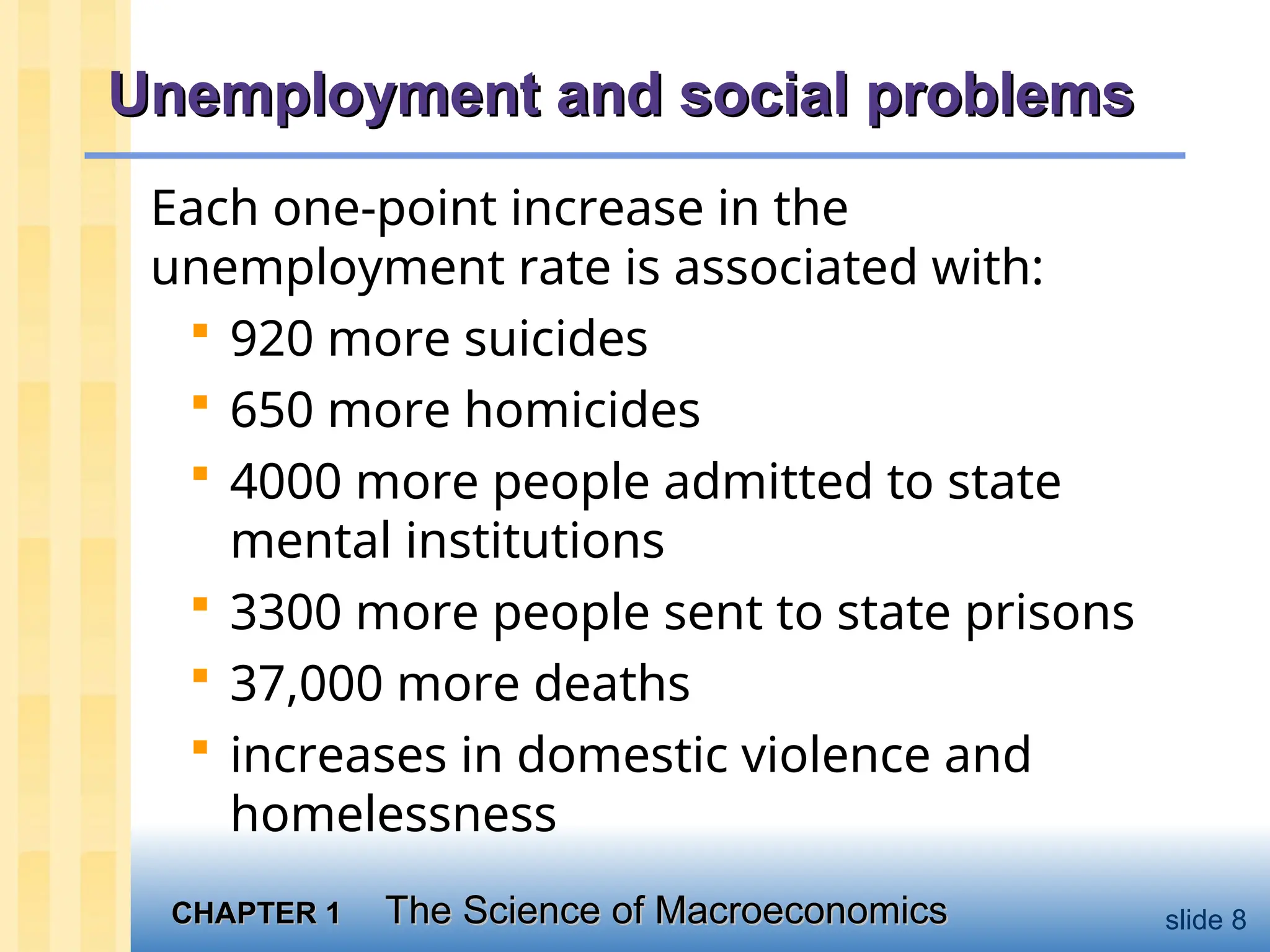
Unemployment and social problems
Unemployment and social problems
Each one-point increase in the
unemployment rate is associated with:
920 more suicides
650 more homicides
4000 more people admitted to state
mental institutions
3300 more people sent to state prisons
37,000 more deaths
increases in domestic violence and
homelessness
9.
CHAPTER 1
CHAPTER 1The Science of Macroeconomics
The Science of Macroeconomics slide 9
Why learn macroeconomics?
Why learn macroeconomics?
1. The macroeconomy affects society’s well-being.
example:
Unemployment and social problems
2. The macroeconomy affects your well-being.
example 1:
Unemployment and earnings growth
example 2:
Interest rates and mortgage payments
10.
CHAPTER 1
CHAPTER 1The Science of Macroeconomics
The Science of Macroeconomics slide 10
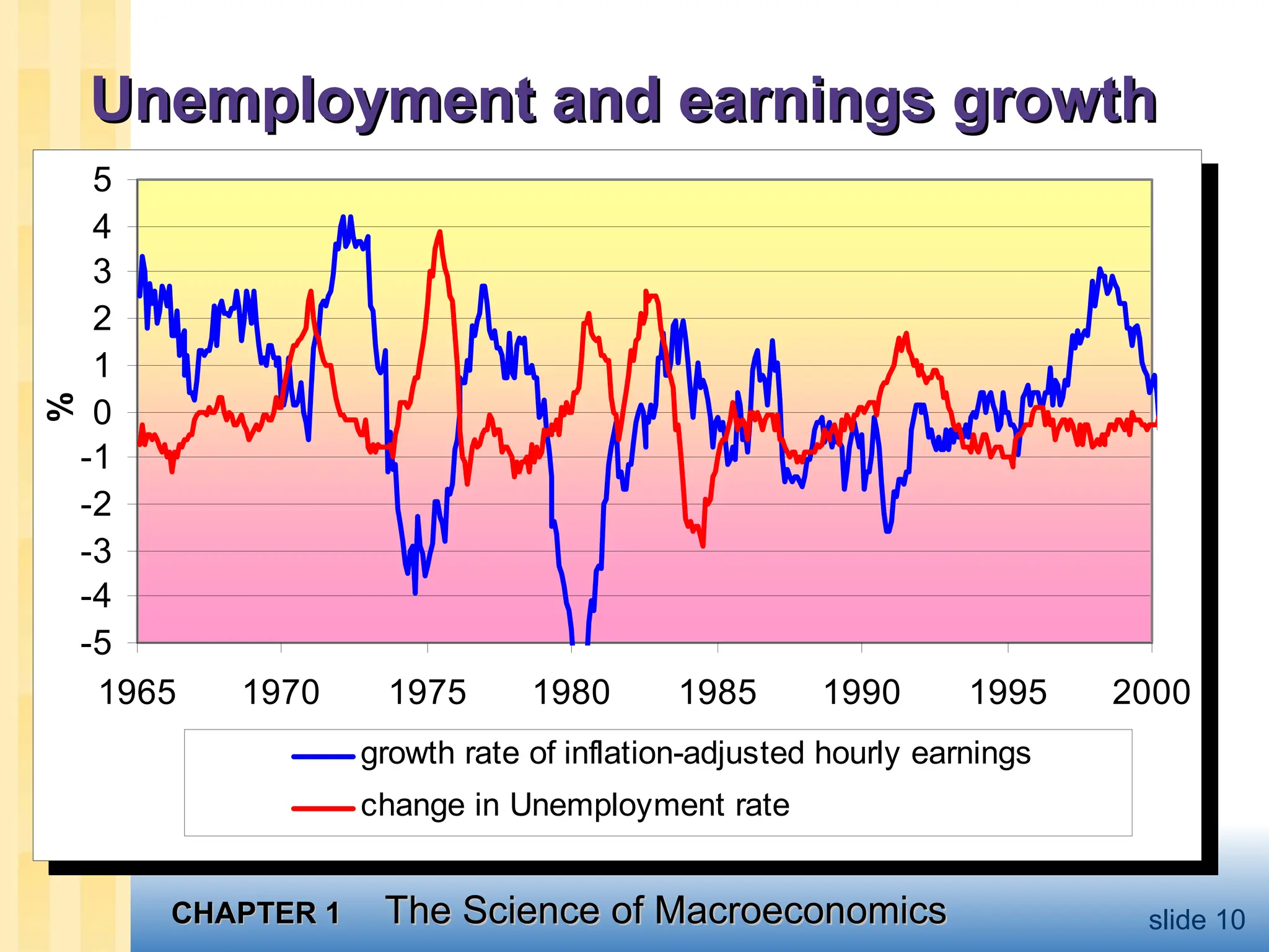
Unemployment and earnings growth
Unemployment and earnings growth
-5
-4
-3
-2
-1
0
1
2
3
4
5
1965 1970 1975 1980 1985 1990 1995 2000
%
growth rate of inflation-adjusted hourly earnings
change in Unemployment rate
11.
CHAPTER 1
CHAPTER 1The Science of Macroeconomics
The Science of Macroeconomics slide 11
Interest rates and mortgage payments
Interest rates and mortgage payments
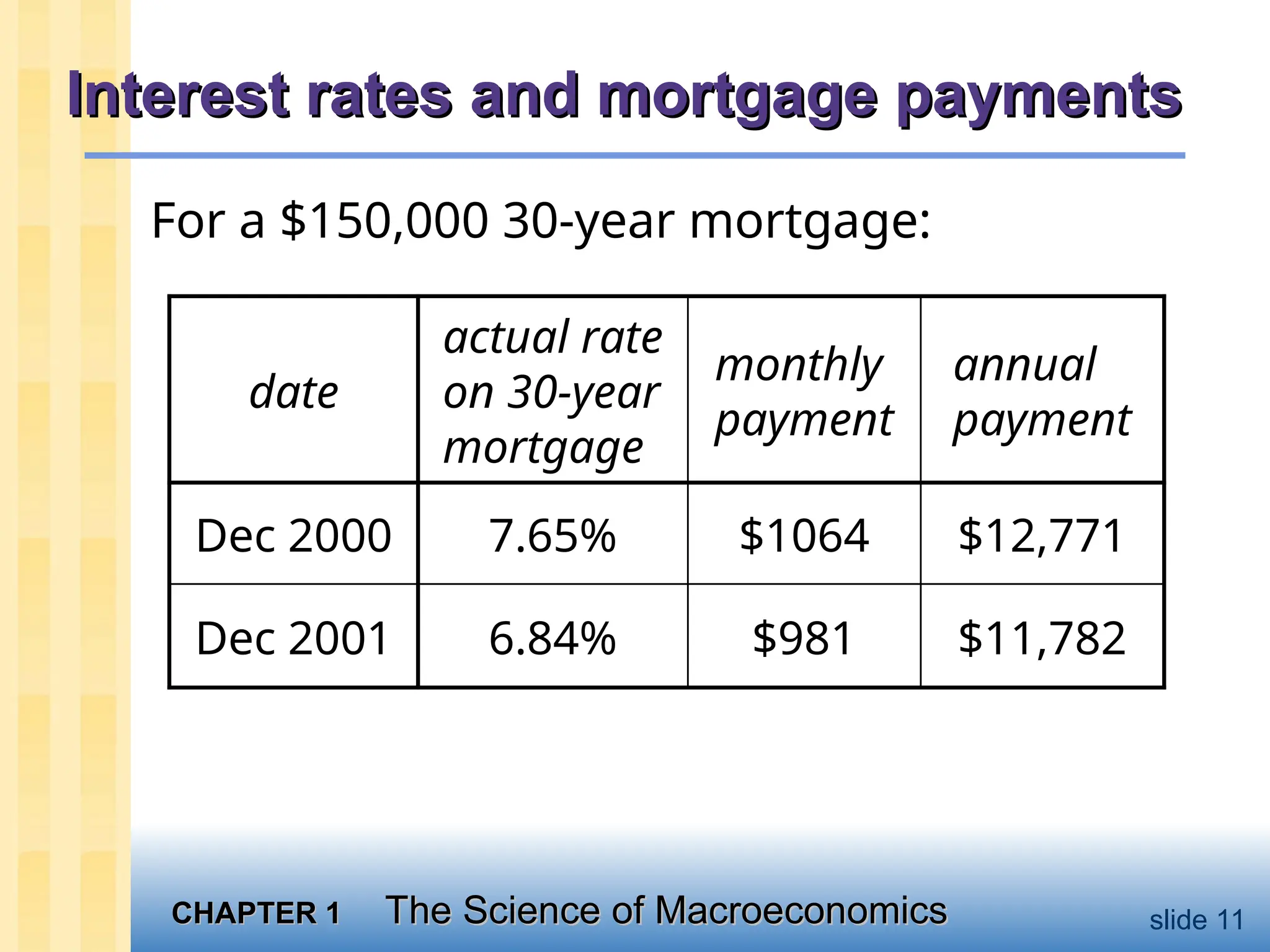
For a $150,000 30-year mortgage:
$11,782
$981
6.84%
Dec 2001
$12,771
$1064
7.65%
Dec 2000
annual
payment
monthly
payment
actual rate
on 30-year
mortgage
date
12.
CHAPTER 1
CHAPTER 1The Science of Macroeconomics
The Science of Macroeconomics slide 12
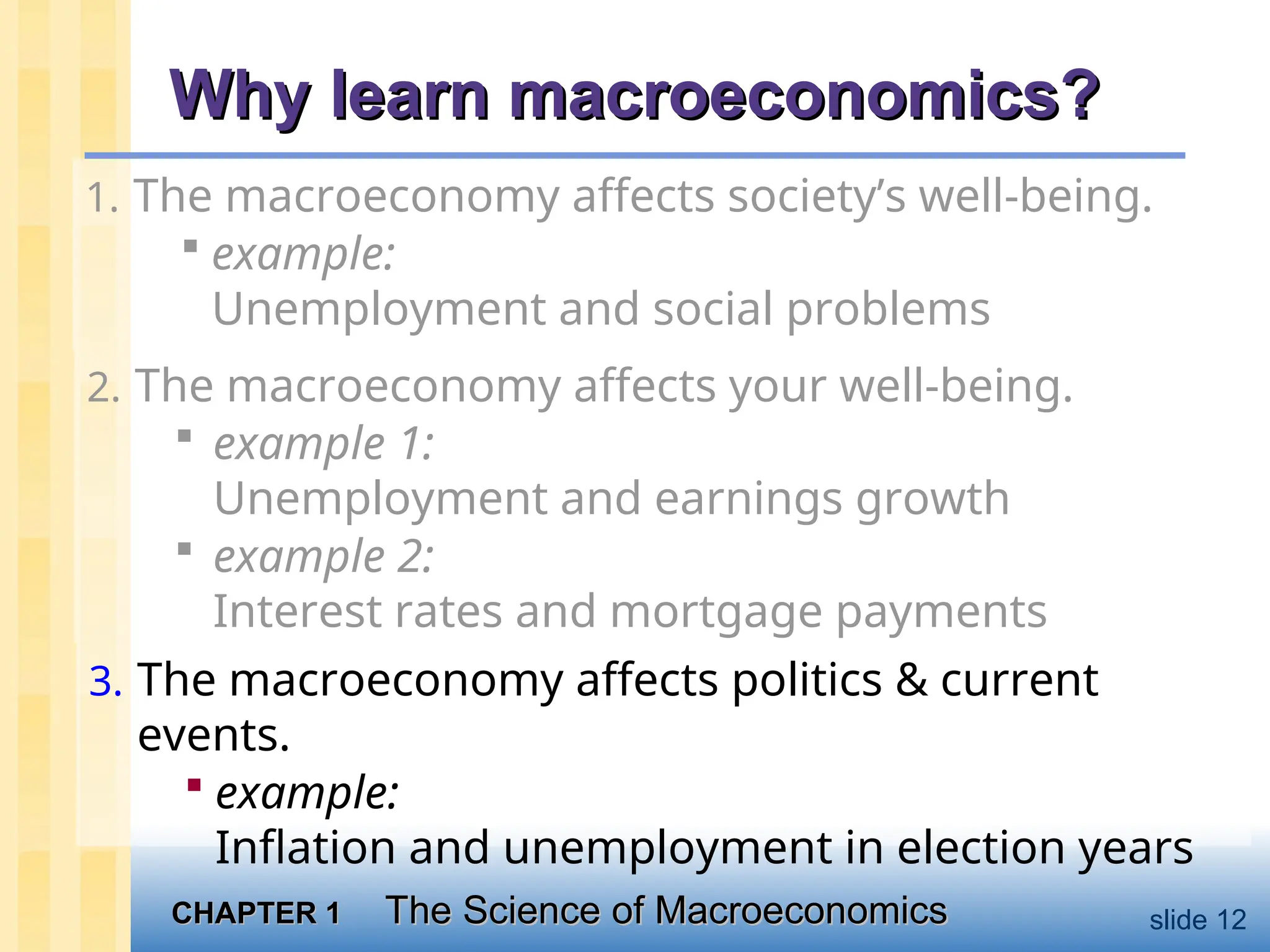
Why learn macroeconomics?
Why learn macroeconomics?
1. The macroeconomy affects society’s well-being.
example:
Unemployment and social problems
2. The macroeconomy affects your well-being.
example 1:
Unemployment and earnings growth
example 2:
Interest rates and mortgage payments
3. The macroeconomy affects politics & current
events.
example:
Inflation and unemployment in election years
13.
CHAPTER 1
CHAPTER 1The Science of Macroeconomics
The Science of Macroeconomics slide 13
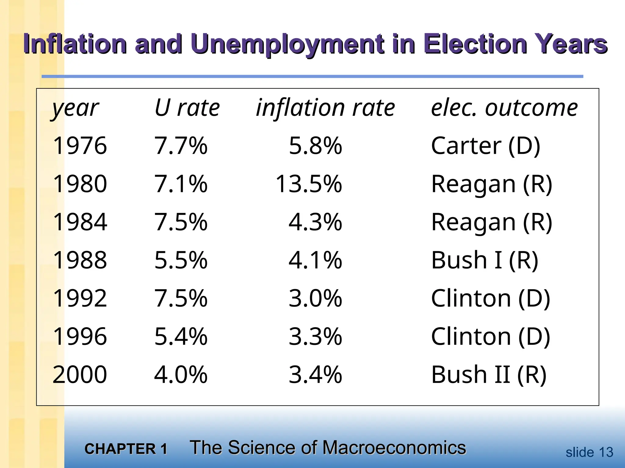
Inflation and Unemployment in Election Years
Inflation and Unemployment in Election Years
year U rate inflation rate elec. outcome
1976 7.7% 5.8% Carter (D)
1980 7.1% 13.5% Reagan (R)
1984 7.5% 4.3% Reagan (R)
1988 5.5% 4.1% Bush I (R)
1992 7.5% 3.0% Clinton (D)
1996 5.4% 3.3% Clinton (D)
2000 4.0% 3.4% Bush II (R)
14.
CHAPTER 1
CHAPTER 1The Science of Macroeconomics
The Science of Macroeconomics slide 14
Economic models
Economic models
…are simplied versions of a more complex
reality
• irrelevant details are stripped away
Used to
• show the relationships between economic
variables
• explain the economy’s behavior
• devise policies to improve economic
performance
15.
CHAPTER 1
CHAPTER 1The Science of Macroeconomics
The Science of Macroeconomics slide 15
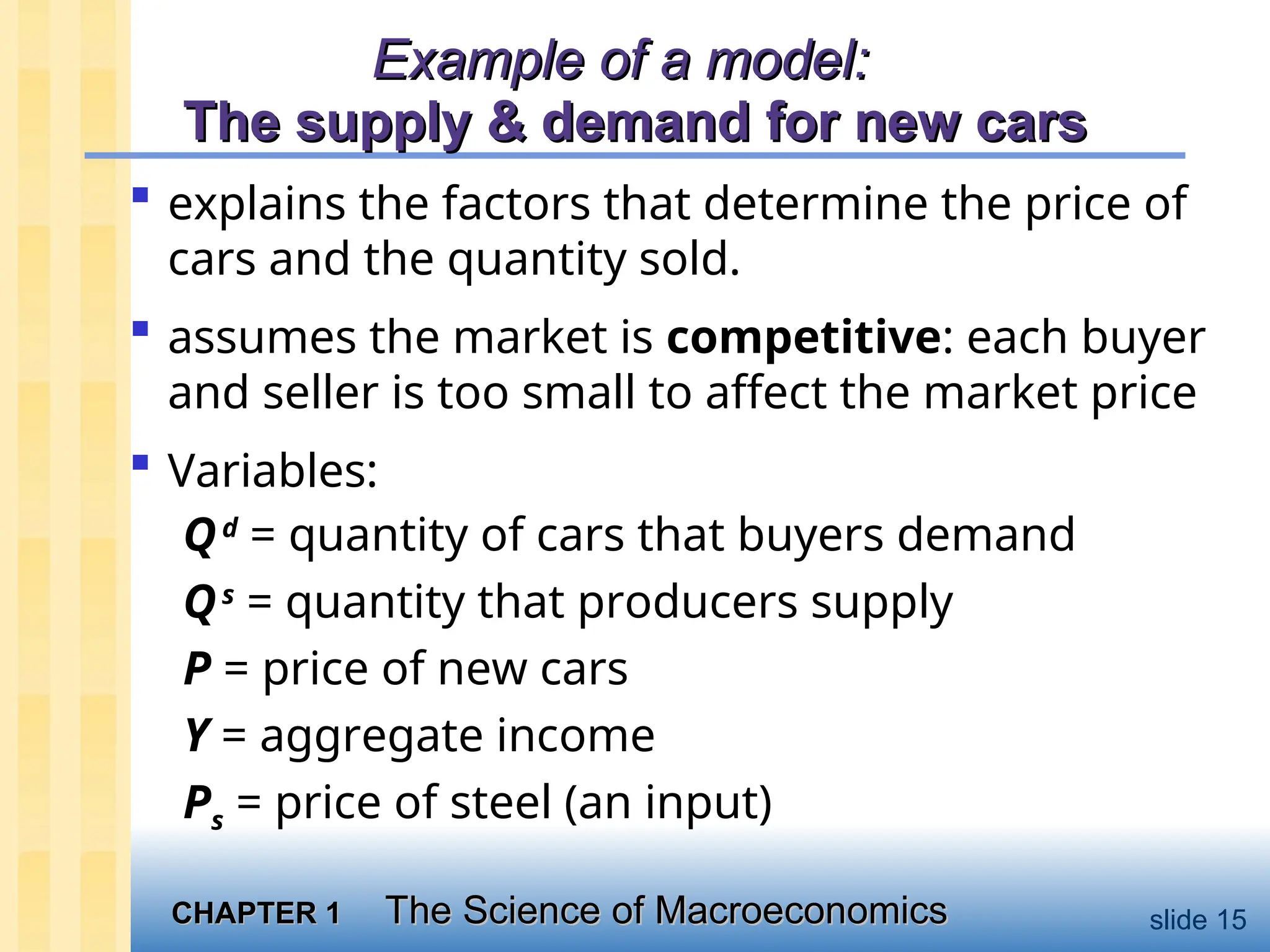
Example of a model:
Example of a model:
The supply & demand for new cars
The supply & demand for new cars
explains the factors that determine the price of
cars and the quantity sold.
assumes the market is competitive: each buyer
and seller is too small to affect the market price
Variables:
Qd
= quantity of cars that buyers demand
Qs
= quantity that producers supply
P = price of new cars
Y = aggregate income
Ps = price of steel (an input)
16.
CHAPTER 1
CHAPTER 1The Science of Macroeconomics
The Science of Macroeconomics slide 16
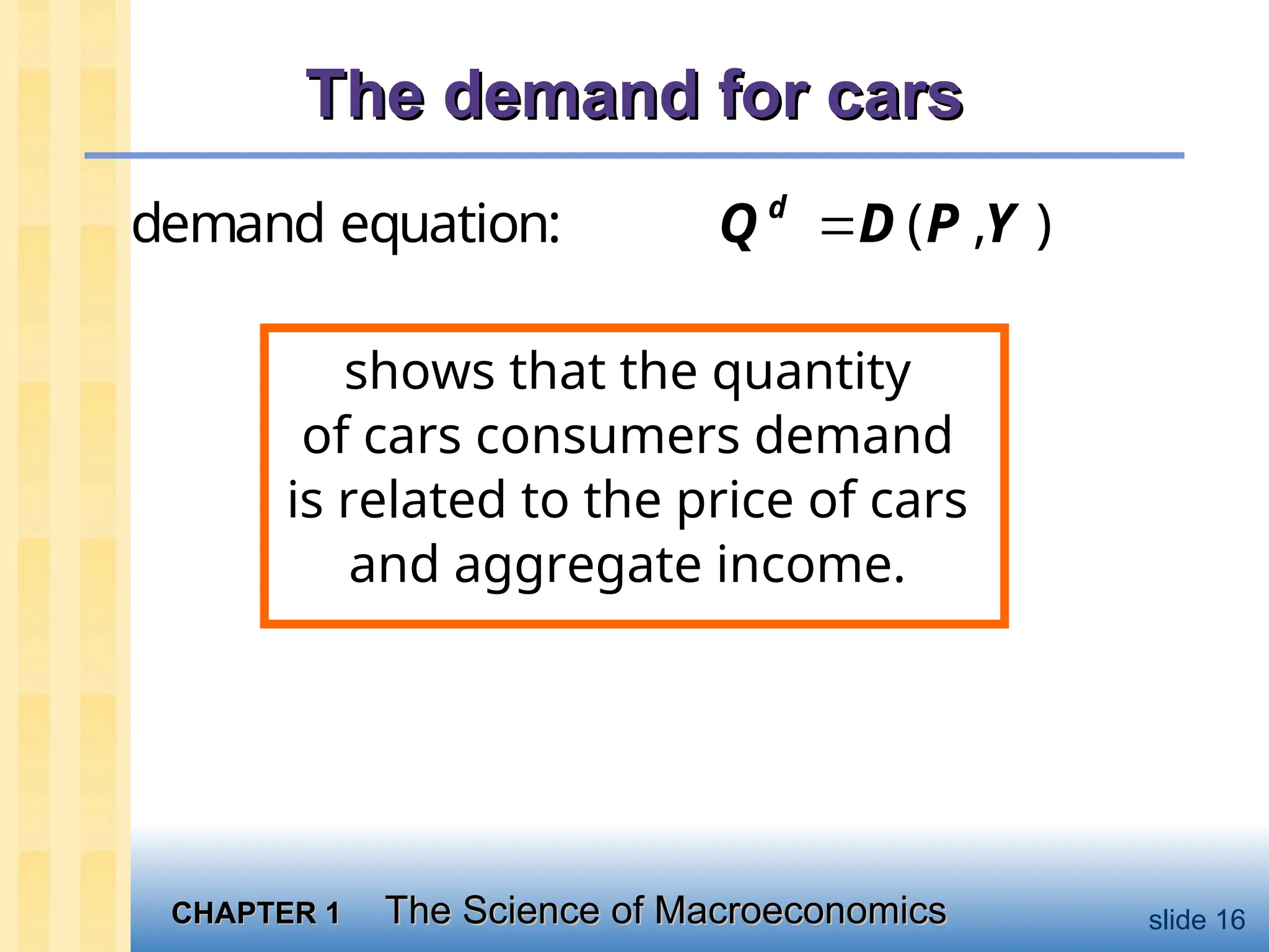
The demand for cars
The demand for cars
shows that the quantity
of cars consumers demand
is related to the price of cars
and aggregate income.
demand equation: ( , )
d
Q D P Y
17.
CHAPTER 1
CHAPTER 1The Science of Macroeconomics
The Science of Macroeconomics slide 17
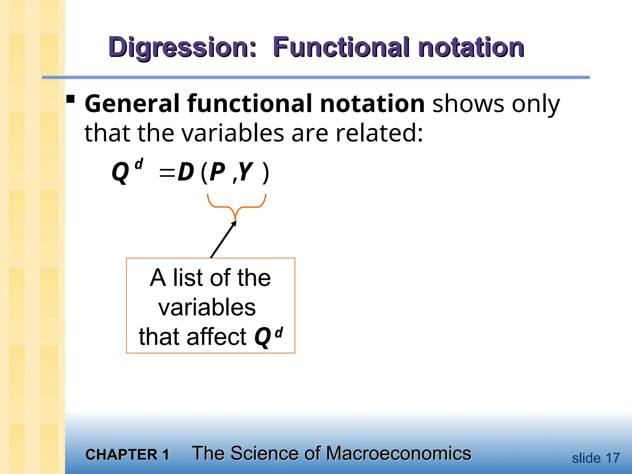
Digression: Functional notation
Digression: Functional notation
General functional notation shows only
that the variables are related:
( , )
d
Q D P Y
A list of the
variables
that affect Qd
18.
CHAPTER 1
CHAPTER 1The Science of Macroeconomics
The Science of Macroeconomics slide 18
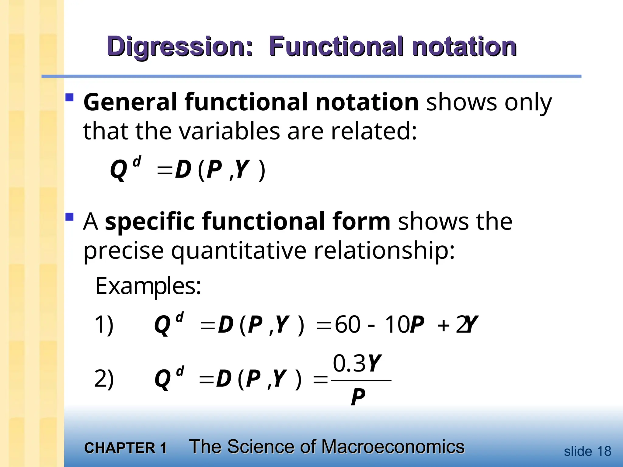
Digression: Functional notation
Digression: Functional notation
General functional notation shows only
that the variables are related:
( , )
d
Q D P Y
A specific functional form shows the
precise quantitative relationship:
Examples:
1) ( , ) 60 10 2
d
Q D P Y P Y
0.3
2) ( , )
d Y
Q D P Y
P
19.
CHAPTER 1
CHAPTER 1The Science of Macroeconomics
The Science of Macroeconomics slide 19
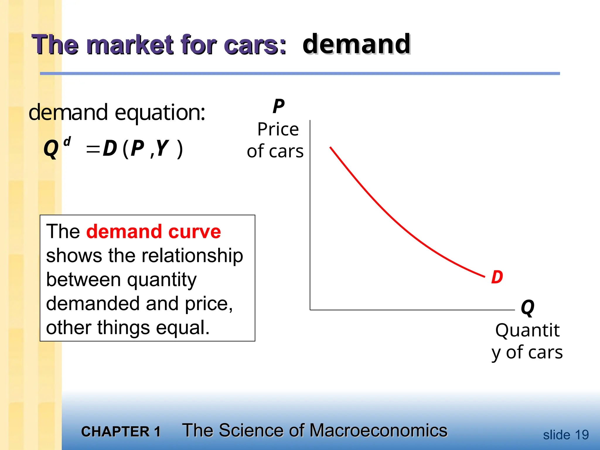
The market for cars:
The market for cars: demand
demand
Q
Quantit
y of cars
P
Price
of cars
D
The demand curve
shows the relationship
between quantity
demanded and price,
other things equal.
demand equation:
( , )
d
Q D P Y
20.
CHAPTER 1
CHAPTER 1The Science of Macroeconomics
The Science of Macroeconomics slide 20
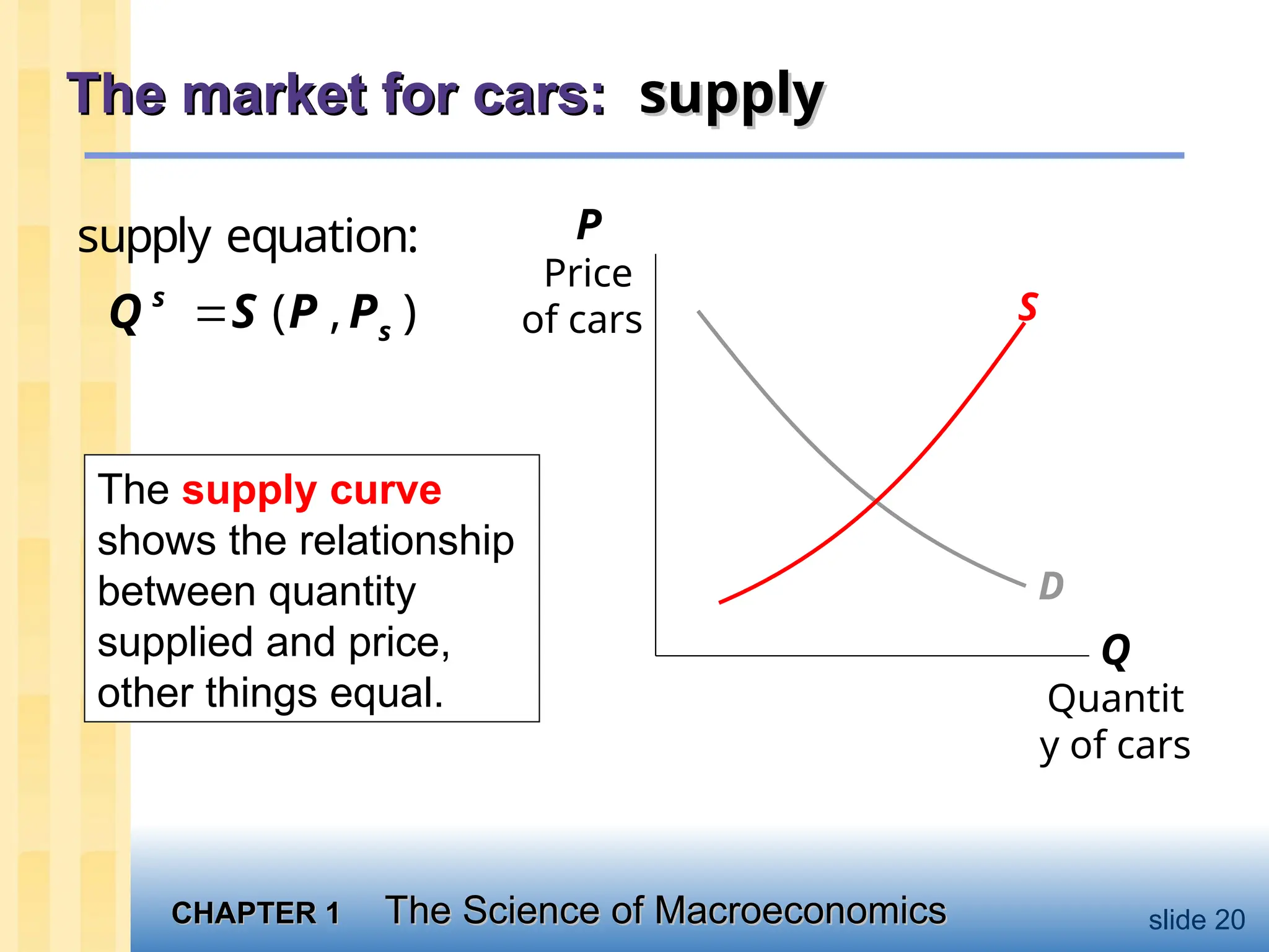
The market for cars:
The market for cars: supply
supply
Q
Quantit
y of cars
P
Price
of cars
D
supply equation:
( , )
s
s
Q S P P S
The supply curve
shows the relationship
between quantity
supplied and price,
other things equal.
21.
CHAPTER 1
CHAPTER 1The Science of Macroeconomics
The Science of Macroeconomics slide 21
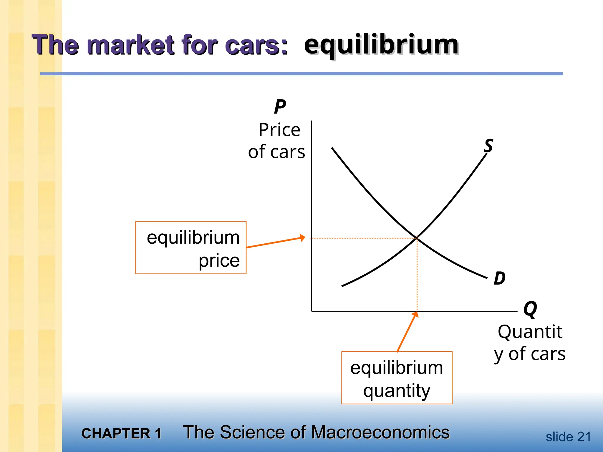
The market for cars:
The market for cars: equilibrium
equilibrium
Q
Quantit
y of cars
P
Price
of cars S
D
equilibrium
price
equilibrium
quantity
22.
CHAPTER 1
CHAPTER 1The Science of Macroeconomics
The Science of Macroeconomics slide 22
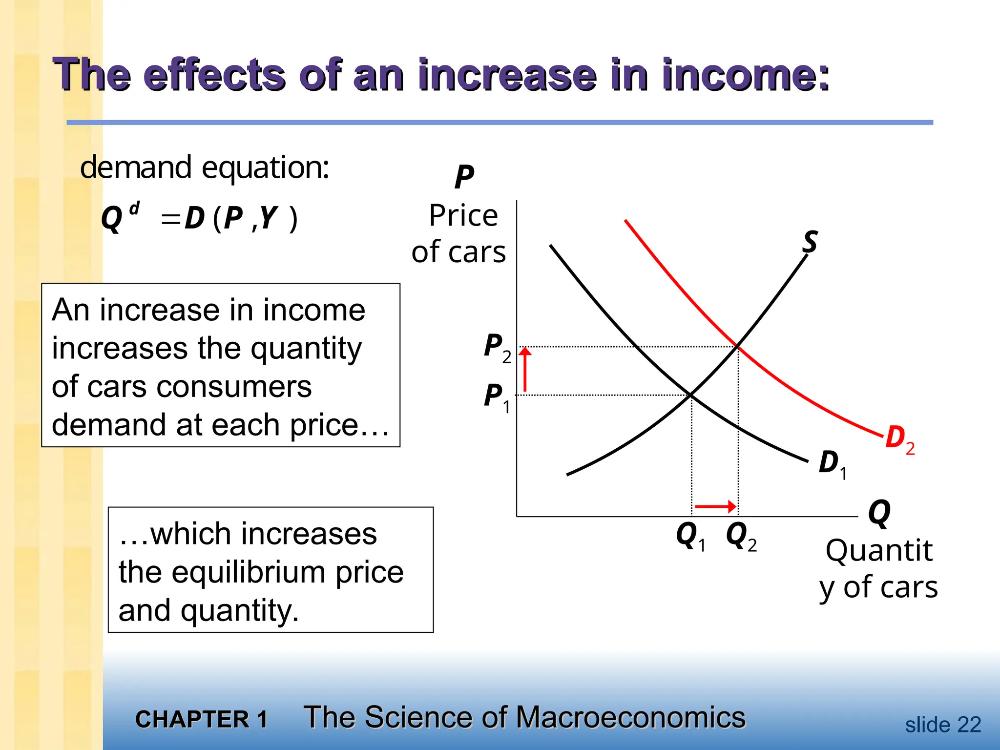
The effects of an increase in income:
The effects of an increase in income:
D2
Q
Quantit
y of cars
P
Price
of cars S
D1
Q1
P1
An increase in income
increases the quantity
of cars consumers
demand at each price…
…which increases
the equilibrium price
and quantity.
P2
Q2
demand equation:
( , )
d
Q D P Y
23.
CHAPTER 1
CHAPTER 1The Science of Macroeconomics
The Science of Macroeconomics slide 23
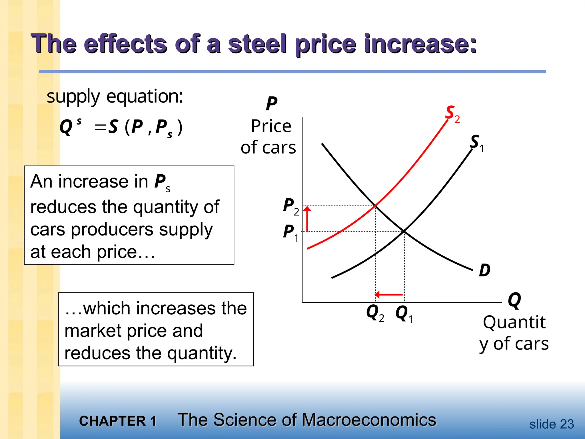
The effects of a steel price increase:
The effects of a steel price increase:
Q
Quantit
y of cars
P
Price
of cars S1
D
Q1
P1
An increase in Ps
reduces the quantity of
cars producers supply
at each price…
…which increases the
market price and
reduces the quantity.
P2
Q2
S2
supply equation:
( , )
s
s
Q S P P
24.
CHAPTER 1
CHAPTER 1The Science of Macroeconomics
The Science of Macroeconomics slide 24
Endogenous vs. exogenous variables:
Endogenous vs. exogenous variables:
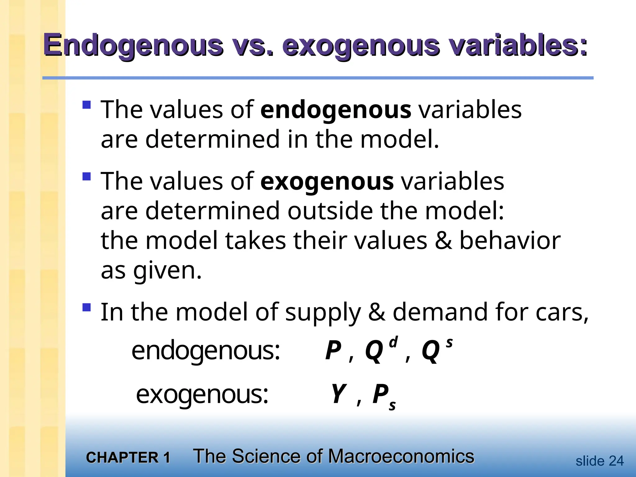
The values of endogenous variables
are determined in the model.
The values of exogenous variables
are determined outside the model:
the model takes their values & behavior
as given.
In the model of supply & demand for cars,
endogenous: , ,
d s
P Q Q
exogenous: , s
Y P
25.
CHAPTER 1
CHAPTER 1The Science of Macroeconomics
The Science of Macroeconomics slide 25
Now you try:
Now you try:
1. Write down demand and supply
equations for wireless phones;
include two exogenous variables
in each equation.
2. Draw a supply-demand graph
for wireless phones.
3. Use your graph to show how a
change in one of your exogenous
variables affects the model’s
endogenous variables.
26.
CHAPTER 1
CHAPTER 1The Science of Macroeconomics
The Science of Macroeconomics slide 26
A Multitude of Models
A Multitude of Models
No one model can address all the issues we
care about. For example,
If we want to know how a fall in
aggregate income affects new car prices,
we can use the S/D model for new cars.
But if we want to know why aggregate
income falls, we need a different model.
27.
CHAPTER 1
CHAPTER 1The Science of Macroeconomics
The Science of Macroeconomics slide 27
A Multitude of Models
A Multitude of Models
So we will learn different models for
studying different issues (e.g.
unemployment, inflation, long-run growth).
For each new model, you should keep track
of
– its assumptions,
– which of its variables are endogenous and
which are exogenous,
– the questions it can help us understand,
– and those it cannot.
28.
CHAPTER 1
CHAPTER 1The Science of Macroeconomics
The Science of Macroeconomics slide 28
Prices: Flexible Versus Sticky
Prices: Flexible Versus Sticky
Market clearing: an assumption that
prices are flexible and adjust to equate
supply and demand.
In the short run, many prices are sticky---
they adjust only sluggishly in response to
supply/demand imbalances.
For example,
– labor contracts that fix the nominal
wage for a year or longer
– magazine prices that publishers change
only once every 3-4 years
29.
CHAPTER 1
CHAPTER 1The Science of Macroeconomics
The Science of Macroeconomics slide 29
Prices: Flexible Versus Sticky
Prices: Flexible Versus Sticky
The economy’s behavior depends partly on
whether prices are sticky or flexible:
If prices are sticky, then demand won’t
always equal supply. This helps explain
– unemployment (excess supply of labor)
– the occasional inability of firms to sell what
they produce
Long run: prices flexible, markets clear,
economy behaves very differently.
30.
CHAPTER 1
CHAPTER 1The Science of Macroeconomics
The Science of Macroeconomics slide 30
Outline of this book:
Outline of this book:
Introductory material (chaps. 1 & 2)
Classical Theory (chaps. 3-6)
How the economy works in the long run,
when prices are flexible
Growth Theory (chaps. 7-8)
The standard of living and its growth rate
over the very long run
Business Cycle Theory (chaps 9-13)
How the economy works in the short run,
when prices are sticky.
31.
CHAPTER 1
CHAPTER 1The Science of Macroeconomics
The Science of Macroeconomics slide 31
Outline of this book:
Outline of this book:
Policy debates (Chaps. 14-15)
Should the government try to smooth
business cycle fluctuations? Is the
government’s debt a problem?
Microeconomic foundations (Chaps. 16-19)
Insights from looking at the behavior of
consumers, firms, and other issues from a
microeconomic perspective.
32.
CHAPTER 1
CHAPTER 1The Science of Macroeconomics
The Science of Macroeconomics slide 32
Chapter summary
Chapter summary
1. Macroeconomics is the study of the
economy as a whole, including
• growth in incomes
• changes in the overall level of prices
• the unemployment rate
2. Macroeconomists attempt to explain the
economy and to devise policies to
improve its performance.
33.
CHAPTER 1
CHAPTER 1The Science of Macroeconomics
The Science of Macroeconomics slide 33
Chapter summary
Chapter summary
3. Economists use different models to
examine different issues.
4. Models with flexible prices describe the
economy in the long run; models with
sticky prices describe economy in the
short run.
5. Macroeconomic events and performance
arise from many microeconomic
transactions, so macroeconomics uses
many of the tools of microeconomics.
34.
CHAPTER 1
CHAPTER 1The Science of Macroeconomics
The Science of Macroeconomics slide 34
Editor's Notes
#1 To the professor:
Much of this chapter is review to students who have taken principles of economics. I’d encourage you to consider one of the following:
1. Spend relatively little time on it (perhaps one 50-minute class session), because it’s perhaps the easiest chapter in the book, and because there often is not quite enough time in the semester to cover all the chapters we’d like to cover.
2. Couple this chapter with some type of classroom activity or discussion, to engage your students, motivate the topic, and set the tone for a great semester. Idea: find two articles from current periodicals with opposing viewpoints on the same issue; bring copies to class; randomly assign students into pairs; in each pair, one student reads one of the articles, the other student reads the other article; allow 15 minutes for students to read their assigned article; then each student gets 5 minutes to teach the content of his or her article to the other student in the pair; then 10 minutes of class discussion.
Note: I’ve added a fair amount of extra material to the PowerPoint presentation of this chapter, especially material that motivates the study of macroeconomics. If you want to get through the chapter more quickly, you might consider cutting some of this additional material.
#3 This slide and the next contain a list of some topical issues that macro can help students understand. Feel free to substitute others as new issues emerge.
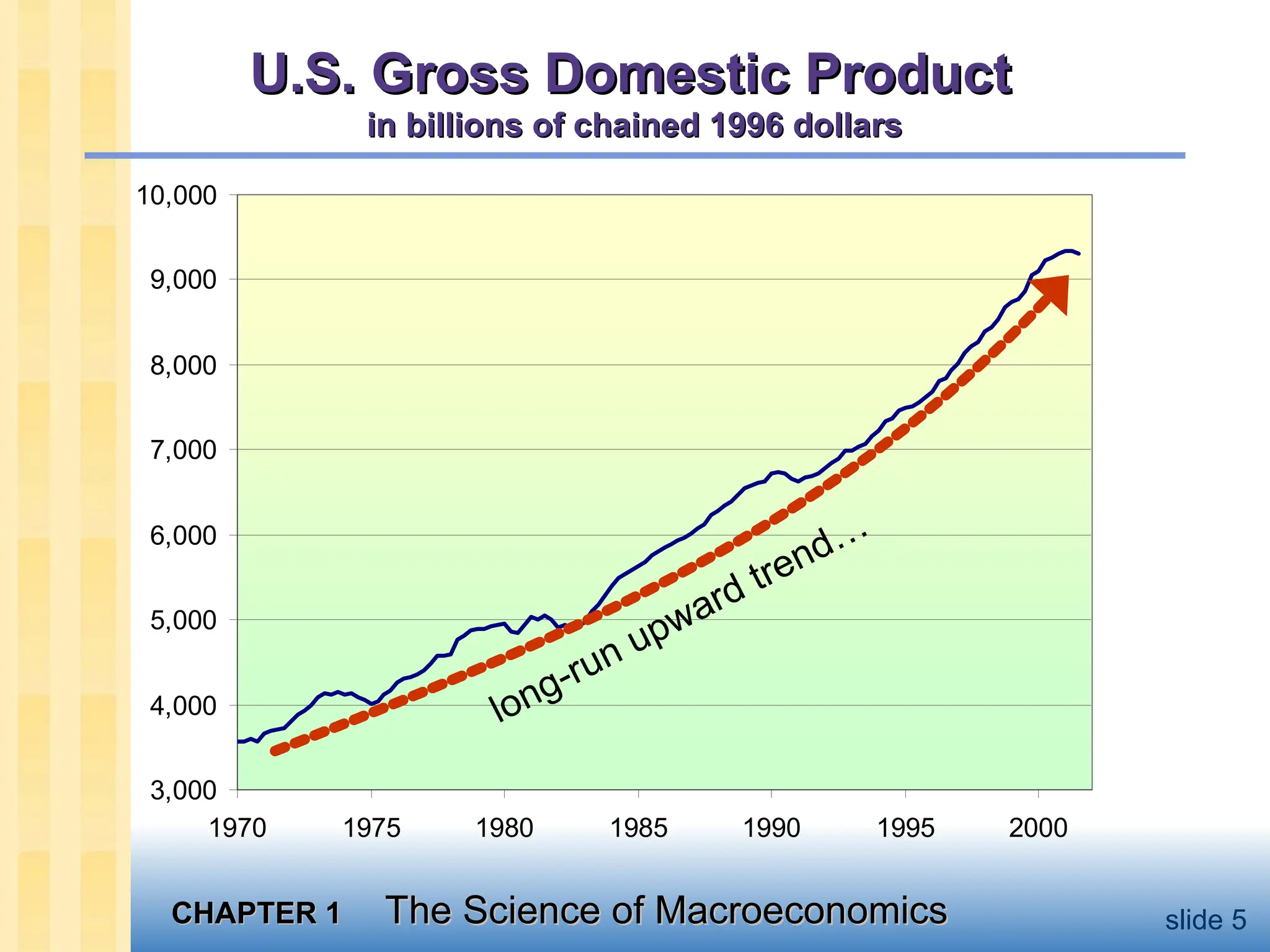
#5 This graph shows data on U.S. Gross Domestic Product. For now, it suffices for students to know that GDP is a measure of the economy’s total output and total income, and that the data in this chart have been adjusted to take out the effects of inflation. (In Chapter 2, students will learn the exact definition of GDP, how it’s measured, and how it’s corrected for inflation).
There are two main points students should get from this graph.
First, over the long run, there’s a clear upward trend. One of the most important issues in macroeconomics is understanding this long run growth: what determines how fast a country grows over the long run, how do government policies affect the growth rate, and how could we achieve faster growth? This topic is critical, because it’s very tightly linked to our standard of living.
(continued next slide….)
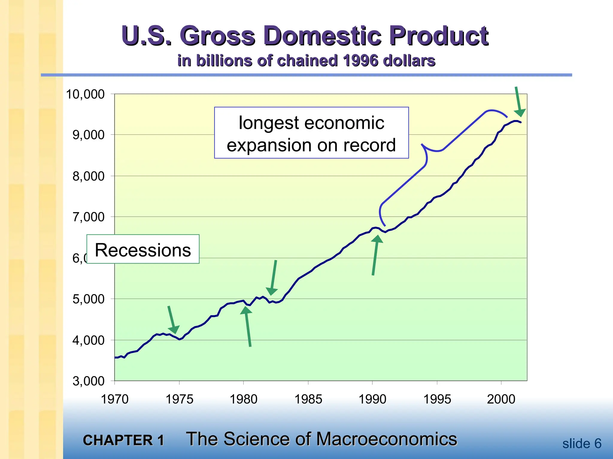
#6 Second, the economy doesn’t always grow smoothly: over the short run, the economy sometimes experiences periods of falling GDP, called recessions. What students see in this graph as little downward blips correspond to periods during which hundreds of thousands of workers lose their jobs.
Periods of rising GDP are called “expansions.” In March 2001, the U.S. completed the longest expansion on record. When the economy is expanding, firms are producing more goods and services, and therefore hiring more workers. Consumer incomes are rising, and consumers are spending more.
#8 Source: Barry Bluestone and Bennett Harrison, The Deindustrialization of America (New York: Basic Books, 1982), Chapter 3, cited in Robert J. Gordon, Macroeconomics, 4th edition (Boston: Little, Brown and Company), p.334. If you know of more recent estimates, please email me so I can update this slide!!! Thanks! (My email address is roncron@unlv.edu)
It might be useful to briefly define the unemployment rate so that students will be able to understand this and the next few slides.
#10 Macroeconomics helps students understand forces that will affect their financial well-being. Here’s an example.
When the unemployment rate is rising, tens or hundreds of thousands of people are losing their jobs. Hopefully our students will not be among them. But the rising unemployment rate even affects those who don’t lose their jobs. As the graph shows, during most years there is a clear negative relationship between the (12-month) change in unemployment and the annual growth rate of real wages. In plain English, rising unemployment is associated with falling (and often negative) wage growth. So when the economy goes into recession, even if our students get to keep their jobs, they will find it much harder to get a raise, and may have to accept a real wage cut.
Students find this relationship intuitive. When unemployment is rising, the supply of workers is rising faster than demand, so wages grow more slowly or even fall. Conversely, falling unemployment gives workers more bargaining power over wages, as it becomes increasingly hard for employers to replace their workers, and increasingly easy for workers to find good opportunities with other companies.
#11 Here’s another example of how the macroeconomy directly affects the pocketbooks of most people, including most of our students after they graduate.
Interest rates are determined by economic factors and by Federal Reserve policy (all of which students will learn about in your course). Rates, in turn, impact the size of our car payments and mortgage payments, which affect how nice of a car or a house we can afford. To illustrate, let’s see how the actual interest rate changes during 2001 affected the typical $150,000 30-year mortgage.
Alan Greenspan and the Federal Reserve reduced interested rates several times in 2001. Because most interest rates tend to move in the same direction, mortgage rates have fallen as well (though not as much as the Fed Funds rate; mortgages are not close substitutes for Federal Funds).
This data shows that people who bought homes at the end of 2001 pay significantly smaller total interest payments per year on their mortgage than people who bought homes just a year earlier. In the example, the difference is almost $1000 per year. You can buy a lot of pizza and compact discs with $1000.
Of course, when inflation is heating up, the Fed raises rates, and then home ownership becomes more costly.
What if your students are renters? Well, changes in mortgage rates affect demand for apartments, since home ownership and renting are substitutes. An increase in mortgage rates will shift demand toward rentals. Then, when it’s time to renew your lease, you’ll find that your landlord has raised your rent. And why shouldn’t she? With high demand for apartments, it would be easy for her to find someone to move in to your apartment if you don’t accept the rent increase.
#13 I’d also suggest you briefly define the inflation rate (as the percentage increase in the cost of living) to help students understand this slide.
Main point of this data: The state of the economy has a huge impact on election outcomes. When the economy is doing poorly, there tends to be a change in the party that controls the White House.
1976: The rates of inflation () and unemployment (u) both high. Incumbent (Ford, R) loses.
1980: u still high, even higher. Incumbent (Carter, D) loses.
1984: u still high, but much lower. Incumbent (Reagan) wins.
1988: the same, u much lower. Incumbent party wins.
1992: low, but u much higher (and was higher yet in 1991). Incumbent loses.
1996: u much lower, incumbent wins.
2000: Economy doing great, and incumbent party candidate (Gore, D) wins majority of popular vote, but loses electoral college to challenger.
#15 Students will realize that the auto market is not competitive. However, if all we want to know is how an increase in the price of steel or a fall in consumer income affects the price and quantity of autos, then it’s fine to use this model.
In general, making unrealistic assumptions is okay, even desirable, if they simplify the analysis without affecting its validity.
#18 We often aren’t concerned with the exact quantitative relationship between variables, so we will often just use the general functional notation.
#30 The portion of the book described on this slide comprises the core material. It is organized around time horizons: the long run (flexible prices), the very long run (growth in capital, the population, and technology itself), and the short run (sticky prices and economic fluctuations).
But wait! There’s more! See the next slide….
#31 All of the chapters listed on this slide are very good, but some instructors find that the semester isn’t always long enough to cover all of this material. Feel free to select chapters from these parts that best match the needs and interests of you and your students.
*** Are you covering Chapter 2 next? The PowerPoint presentation for Chapter 2 includes some in-class exercises to immediately reinforce concepts as they are presented. These exercises also help break up the lecture into smaller pieces. If you’d like to try them, please ask your students to bring calculators to the next class meeting.