The 2024 Level 1 formula sheet provides essential formulas and calculations necessary for the CFA program curriculum, including financial calculator keys and various mathematical concepts such as present and future value, probability, and regression analysis. It includes information on economic indicators, monetary and fiscal policy, and key financial ratios, while emphasizing the importance of using this document alongside the core readings. This document is copyrighted material from the CFA Institute and should be utilized for educational purposes only.

1. 2024
Level 1 - Formula Sheet
This document should be used in conjunction with the corresponding readings in the 2024 Level 1 CFA® Program curriculum. Some of the graphs, charts, tables, examples, and figures
are copyright 2022, CFA Institute. Reproduced and republished with permission from CFA Institute. All rights reserved.
Required disclaimer: CFA Institute does not endorse, promote, or warrant accuracy or quality of the products or services offered by MarkMeldrum.com. CFA Institute, CFA®, and
Chartered Financial Analyst® are trademarks owned by CFA Institute.
© markmeldrum.com. All rights reserved.
M.M140077214.

2. Quantitative Methods
Financial Calculator Keys
N = Number of Compounding Periods
I/Y = Interest Rate per Year
*In whole numbers (i.e. 5% is entered as 5)
PV = Present Value
PMT = Payment
FV = Future Value
End-of-period payments
*Used for regular annuity
2nd [BGN]
2nd Enter
Display END
Beginning-of-period payments
*Used for annuity due
2nd [BGN]
2nd Enter
Display BGN
Cash Flow Worksheet
CFn = cash flow at time period n
Using the arrow keys and the ENTER key to input
cash flow amounts and their frequencies.
Solving for net present value: the NPV key will
prompt you to input a discount rate (I). Then
pressing the down key and CPT to find the NPV.
Solving for the internal rate of return: use the IRR
key and press CPT.
ICONV
Used to calculate effective rates
Nom = Nominal Rate
C/Y = Compounding Frequency
EFF-> CPT = outputs effective rate
Other Helpful Keys
STO = allows you to store values.
RCL = allows you to recall stored values.
FORMAT
2nd + FORMAT allows you to change the number of
decimal places displayed on the calculator.
DATA & STAT
Computes multiple values (mean, standard
deviation, etc...)
2nd + DATA allows you to your input variables. Once
inputted, exit the page, and click 2nd + STAT to find
the computed outputs. Use the down arrow keys
scroll through the various outputs.
Future Value (FV) of a single cash flow
𝐹𝑉 = 𝑃𝑉 × (1 + 𝑟)𝑁
Present Value (PV) of a single cash flow
𝑃𝑉 =
𝐹𝑉
(1 + 𝑟)𝑁
Present Value (PV) of Perpetuity
𝑃𝑉(𝑝𝑒𝑟𝑝𝑒𝑡𝑢𝑖𝑡𝑦) =
𝐴
𝑟
𝐴 = 𝑃𝑎𝑦𝑚𝑒𝑛𝑡 𝑎𝑚𝑜𝑢𝑛𝑡
Future Value (FV) with continuous
compounding
𝐹𝑉𝑁 = 𝑃𝑉𝑒𝑟𝑠𝑁
Effective Annual Rate (EAR)
𝐸𝐴𝑅 = (1 + 𝑃𝑒𝑟𝑖𝑜𝑑𝑖𝑐 𝑟𝑎𝑡𝑒)𝑚
− 1
𝑃𝑒𝑟𝑖𝑜𝑑𝑖𝑐 𝑟𝑎𝑡𝑒
=
𝑆𝑡𝑎𝑡𝑒𝑑 𝐴𝑛𝑛𝑢𝑎𝑙 𝑅𝑎𝑡𝑒
𝑁𝑢𝑚𝑏𝑒𝑟 𝑜𝑓 𝐶𝑜𝑚𝑝𝑜𝑢𝑛𝑑𝑖𝑛𝑔 𝑃𝑒𝑟𝑖𝑜𝑑𝑠 𝑂𝑛𝑒 𝑌𝑒𝑎𝑟
𝑚 = 𝑁𝑢𝑚𝑏𝑒𝑟 𝑜𝑓 𝐶𝑜𝑚𝑝𝑜𝑢𝑛𝑑𝑖𝑛𝑔 𝑃𝑒𝑟𝑖𝑜𝑑𝑠 𝑂𝑛𝑒 𝑌𝑒𝑎𝑟
EAR with continuous compounding
𝐸𝐴𝑅 = 𝑒𝑟𝑠 − 1
Relative Frequency
Relative Frequency
=
𝐴𝑏𝑠𝑜𝑙𝑢𝑡𝑒 𝑓𝑟𝑒𝑞𝑢𝑒𝑛𝑐𝑦 𝑜𝑓 𝑒𝑎𝑐ℎ 𝑖𝑛𝑡𝑒𝑟𝑣𝑎𝑙
𝑇𝑜𝑡𝑎𝑙 𝑛𝑢𝑚𝑏𝑒𝑟 𝑜𝑓 𝑜𝑏𝑠𝑒𝑟𝑣𝑎𝑡𝑖𝑜𝑛𝑠
Cumulative Relative Frequency
Cumulative Relative Frequency
= 𝐴𝑑𝑑 𝑡ℎ𝑒 𝑟𝑒𝑙𝑎𝑡𝑖𝑣𝑒 𝑓𝑟𝑒𝑞𝑢𝑒𝑛𝑐𝑖𝑒𝑠 𝑤ℎ𝑖𝑙𝑒 𝑝𝑟𝑜𝑐𝑒𝑒𝑑𝑖𝑛𝑔
𝑓𝑟𝑜𝑚 𝑡ℎ𝑒 𝑓𝑖𝑟𝑠𝑡 𝑡𝑜 𝑡ℎ𝑒 𝑙𝑎𝑠𝑡 𝑖𝑛𝑡𝑒𝑟𝑣𝑎𝑙
Arithmetic Mean
x
̅ =
∑ 𝑋
𝑛
𝑡=1
𝑁
Median
In an ordered sample of n items:
For even number of observations
= Mean of values
𝑛
2
&
𝑛 + 2
2
For odd number of observations =
𝑛 + 1
2
Mode
the most frequently occurring value in a distribution
QM (1/14) QM (2/14) QM (3/14)
M.M140077214.

3. Weighted Average Mean
X
̅𝑤 = ∑ 𝑤𝑖 × 𝑋𝑖
𝑛
𝑖=1
Geometric Mean
G = √(1 + 𝑟1)(1 + 𝑟2)… (1 + 𝑟𝑛)
𝑛
with 𝑟𝑖 ≥ 0 for i = 1,2, … , n
Harmonic Mean
HM =
n
∑ (
1
𝑋𝑖
)
𝑛
𝑖=1
with X𝑖 > 0 for i = 1,2, … , n
Mean Absolute Deviation
MAD =
∑ |𝑥𝑖 − 𝑥̅|
𝑛
𝑖=1
𝑛
Percentile
Percentile = Ly = (n + 1) ×
y
100
Quartile =
Distribution
4
Quintile =
Distribution
5
Decile =
Distribution
10
Range
Range = Maximum value – Minimum value
Population Variance
𝜎2
=
∑ (𝑥𝑖 − 𝜇)2
𝑁
𝑖=1
𝑁
Sample Variance
𝑠2
=
∑ (𝑥𝑖 − 𝑥̅)2
𝑛
𝑖=1
𝑛 − 1
Standard Deviation
Square root of the variance value
Sample Target Semi-Deviation
𝑠Target =√ ∑
(𝑋𝑖 − 𝐵)2
𝑛 − 1
𝑛
𝑓𝑜𝑟 𝑎𝑙𝑙 𝑋𝑖≤ 𝐵
where B is the target and n is the total number of
sample observations.
Coefficient of Variation
𝐶𝑉 =
𝑆𝑡𝑎𝑛𝑑𝑎𝑟𝑑 𝐷𝑒𝑣𝑖𝑎𝑡𝑖𝑜𝑛 𝑜𝑓 𝑥
𝐴𝑣𝑒𝑟𝑎𝑔𝑒 𝑉𝑎𝑙𝑢𝑒 𝑜𝑓 𝑥
=
𝑠𝑥
𝑥̅
Skewness
Positive Skew; Mean > Median > Mode
Negative Skew; Mean < Median < Mode
Probability Stated as Odds
𝑂𝑑𝑑𝑠 𝑓𝑜𝑟 𝑎𝑛 𝐸𝑣𝑒𝑛𝑡 ′𝐸′ =
𝑃(𝐸)
1 − 𝑃(𝐸)
𝑂𝑑𝑑𝑠 𝑎𝑔𝑎𝑖𝑛𝑠𝑡 𝑎𝑛 𝐸𝑣𝑒𝑛𝑡 ′𝐸′ =
1 − 𝑃(𝐸)
𝑃(𝐸)
Probability of A or B
𝑃(𝐴 𝑜𝑟 𝐵) = 𝑃(𝐴) + 𝑃(𝐵) − 𝑃(𝐴𝐵)
Joint Probability of Two Events
𝑃(𝐴𝐵) = 𝑃(𝐴|𝐵) × 𝑃(𝐵)
Conditional Probability of A given B
𝑃(𝐴|𝐵) =
𝑃(𝐴𝐵)
𝑃(𝐵)
Joint Probability of any number of
independent events
𝑃(𝐴𝐵𝐶𝐷𝐸) = 𝑃(𝐴) × 𝑃(𝐵) × 𝑃(𝐶) × 𝑃(𝐷)
× 𝑃(𝐸)
Total Probability Rule
𝑃(𝐴) = 𝑃(𝐴|𝐵1) × 𝑃(𝐵1) + 𝑃(𝐴|𝐵2) × 𝑃(𝐵2)
+ 𝑃(𝐴|𝐵3) × 𝑃(𝐵3)
+ ⋯ 𝑃(𝐴|𝐵𝑛) × 𝑃(𝐵𝑛)
Expected Value of a Random Variable
𝐸(𝑋) = 𝑃(𝑋1)𝑋1 + 𝑃(𝑋2)𝑋2+. . . 𝑃(𝑋𝑛)𝑋𝑛 = ∑ 𝑃(𝑋𝐼)𝑋𝑖
𝑛
𝑖=1
Variance of a Random Variable
𝜎2
(𝑋) = ∑ 𝑃(𝑋𝑖)
𝑛
𝑖=1
[𝑋𝑖 − 𝐸(𝑋)]2
QM (4/14) QM (5/14) QM (6/14)
M.M140077214.

4. Portfolio Expected Return
𝐸(𝑅𝑝) = 𝑤1̇ 𝐸(𝑅1̇ ) + 𝑤2̇ 𝐸(𝑅2̇ ) + 𝑤3𝐸(𝑅3) … 𝑤𝑛𝐸(𝑅𝑛̇ )
Portfolio Variance
𝑣𝑎𝑟(𝑅𝑃) = 𝑤𝐴
2
𝜎2(𝑅𝐴) + 𝑤𝐵
2
𝜎2(𝑅𝐵)
+ 2𝑤𝐴𝑤𝐵𝜎(𝑅𝐴)𝜎(𝑅𝐵)𝜌(𝑅𝐴, 𝑅𝐵)
Covariance
𝑐𝑜𝑣(𝑅1,𝑅𝑗) = 𝐸[(𝑅𝑖 − 𝐸(𝑅𝑖̇)(𝑅𝑗 − 𝐸(𝑅𝑗̇)]
Correlation
𝜌(𝑅𝑖, 𝑅𝑗) =
𝑐𝑜𝑣(𝑅𝑖, 𝑅𝑗)
𝜎(𝑅𝑖)𝜎(𝑅𝑗)
Bayes’ Formula
𝑃(𝐸𝑣𝑒𝑛𝑡|𝐼𝑛𝑓𝑜𝑟𝑚𝑎𝑡𝑖𝑜𝑛)
=
𝑃(𝐼𝑛𝑓𝑜𝑟𝑚𝑎𝑡𝑖𝑜𝑛|𝐸𝑣𝑒𝑛𝑡)
𝑃(𝐼𝑛𝑓𝑜𝑟𝑚𝑎𝑡𝑖𝑜𝑛)
× 𝑃(𝐸𝑣𝑒𝑛𝑡)
Multiplication Rule of Counting
n! = n(n − 1)(n − 2)(n − 3) … 1
Multinomial Formula for Labeling
Problems
n! =
n!
n1! n2! … nk!
Combination Formula
# of ways we can choose r objects from a total of n objects,
when order does not matter.
nCr =
n!
(n − r)! r!
Permutation Formula
# of ways that we can choose r objects from a total of n
objects, when order does matter.
nPr =
n!
(n − r)!
Probabilities for a Random Variable given
its Cumulative Distribution Function
To find F(x), sum up, or cumulate, values of the
probability function for all outcomes less than or
equal to x.
Probabilities given the Discrete Uniform
Function
𝐶𝑢𝑚𝑢𝑙𝑎𝑡𝑖𝑣𝑒 𝑑𝑖𝑠𝑡𝑟𝑖𝑏𝑢𝑡𝑖𝑜𝑛 𝑓𝑢𝑛𝑐𝑡𝑖𝑜𝑛 𝑓𝑜𝑟 𝑡ℎ𝑒 𝑛𝑡ℎ 𝑜𝑢𝑡𝑐𝑜𝑚𝑒
𝐹(𝑋𝑛) = 𝑛𝑃(𝑋)
Probability function for a Binomial
Random Variable
𝑃𝑟𝑜𝑏𝑎𝑏𝑖𝑙𝑖𝑡𝑦 𝑜𝑓𝑥 𝑠𝑢𝑐𝑐𝑒𝑠𝑠𝑒𝑠 𝑖𝑛 𝑛 𝑡𝑟𝑖𝑎𝑙𝑠
=
n!
(n − x)! x!
× 𝑝𝑥(1 − 𝑝)𝑛−𝑥
Expected Value and Variance of a
Binomial Random Variable
𝐸𝑥𝑝𝑒𝑐𝑡𝑒𝑑 𝑉𝑎𝑙𝑢𝑒 𝑜𝑓 𝑋 = nP
𝑉𝑎𝑟𝑖𝑎𝑛𝑐𝑒 𝑜𝑓 𝑋 = nP(1 − p)
Continuous Uniform Distribution
𝑓(𝑥) = {
1
𝑏 − 𝑎
𝑓𝑜𝑟 𝑎 < 𝑥 < 𝑏 𝑜𝑟 0
𝐹(𝑥) =
𝑥 − 𝑎
𝑏 − 𝑎
𝑓𝑜𝑟 𝑎 < 𝑥 < 𝑏
Standardizing a Random Normal Variable
𝑍 =
𝑋 − µ
𝜎
approximately…
50% 𝑜𝑓 𝑎𝑙𝑙 𝑜𝑏𝑠𝑒𝑟𝑣𝑎𝑡𝑖𝑜𝑛𝑠 𝑓𝑎𝑙𝑙 𝑤𝑖𝑡ℎ𝑖𝑛 𝜇 ± (2 ∕ 3)𝜎
68% 𝑜𝑓 𝑎𝑙𝑙 𝑜𝑏𝑠𝑒𝑟𝑣𝑎𝑡𝑖𝑜𝑛𝑠 𝑓𝑎𝑙𝑙 𝑤𝑖𝑡ℎ𝑖𝑛 𝜇 ± 1𝜎
95% 𝑜𝑓 𝑎𝑙𝑙 𝑜𝑏𝑠𝑒𝑟𝑣𝑎𝑡𝑖𝑜𝑛𝑠 𝑓𝑎𝑙𝑙 𝑤𝑖𝑡ℎ𝑖𝑛 𝜇 ± 2𝜎
99% 𝑜𝑓 𝑎𝑙𝑙 𝑜𝑏𝑠𝑒𝑟𝑣𝑎𝑡𝑖𝑜𝑛𝑠 𝑓𝑎𝑙𝑙 𝑤𝑖𝑡ℎ𝑖𝑛 𝜇 ± 3𝜎
Safety-First Ratio
𝑆𝐹𝑅𝑎𝑡𝑖𝑜 =
[𝐸(𝑅𝑝) − 𝑅𝑙)]
𝜎𝑝
Portfolio with the highest ratio is preferred
Continuously Compounded Return
from t = 0 to t = 1
𝑟0,1 = ln(
𝑆1
𝑆0
)
Degrees of Freedom of Student’s
T-distribution
𝑑𝑓 = 𝑛𝑢𝑚𝑏𝑒𝑟 𝑜𝑓 𝑠𝑎𝑚𝑝𝑙𝑒 𝑜𝑏𝑠𝑒𝑟𝑣𝑎𝑡𝑖𝑜𝑛𝑠 − 1 = 𝑛 − 1
Standard Error of the Sample Mean
(σ known)
𝜎𝑋 =
σ
√n
(σ unknown)
𝑠𝑥 =
s
√n
QM (7/14) QM (8/14) QM (9/14)
M.M140077214.

5. Normally Distributed Population with
Known Variance
𝐶𝑜𝑛𝑓𝑖𝑑𝑒𝑛𝑐𝑒 𝑖𝑛𝑡𝑒𝑟𝑣𝑎𝑙𝑠 = 𝑋
̅ ± 𝑧𝜎/2 × (
σ
√n
)
𝑧𝜎/2
≅ 1.65 𝑓𝑜𝑟 90% 𝐶𝑜𝑛𝑓𝑖𝑑𝑒𝑛𝑐𝑒 𝐼𝑛𝑡𝑒𝑟𝑣𝑎𝑙, 5% 𝑖𝑛 𝑒𝑎𝑐ℎ 𝑡𝑎𝑖𝑙
𝑧𝜎/2
= 1.96 𝑓𝑜𝑟 95% 𝐶𝑜𝑛𝑓𝑖𝑑𝑒𝑛𝑐𝑒 𝐼𝑛𝑡𝑒𝑟𝑣𝑎𝑙, 2.5% 𝑖𝑛 𝑒𝑎𝑐ℎ 𝑡𝑎𝑖𝑙
𝑧𝜎/2
≅ 2.58 𝑓𝑜𝑟 99% 𝐶𝑜𝑛𝑓𝑖𝑑𝑒𝑛𝑐𝑒 𝐼𝑛𝑡𝑒𝑟𝑣𝑎𝑙, 0.5% 𝑖𝑛 𝑒𝑎𝑐ℎ 𝑡𝑎𝑖𝑙
Large sample, Population Variance
Unknown
𝐶𝑜𝑛𝑓𝑖𝑑𝑒𝑛𝑐𝑒 𝑖𝑛𝑡𝑒𝑟𝑣𝑎𝑙𝑠 = 𝑋
̅ ± 𝑧𝛼/2 × (
s
√n
)
Small sample, Population Variance
Unknown
𝐶𝑜𝑛𝑓𝑖𝑑𝑒𝑛𝑐𝑒 𝑖𝑛𝑡𝑒𝑟𝑣𝑎𝑙𝑠 = 𝑋
̅ ± 𝑡𝛼/2 × (
s
√n
)
Type I and II Errors
Type I – Reject H0 when true
Type II – Accept H0 when false
Power of a Test
1 − 𝑃(𝑇𝑦𝑝𝑒 𝐼𝐼 𝑒𝑟𝑟𝑜𝑟)
Test of a Single Mean
𝑧 =
𝑋
̅ − 𝜇0
𝜎
√𝑛
⁄
or 𝑡𝑛−1 =
𝑋
̅ − 𝜇0
𝑠
√𝑛
⁄
Test of the Difference in Means
(Equal Variances)
𝑡 =
(𝑋
̅1 − 𝑋
̅2) − (𝜇1 − 𝜇2)
(
𝑠𝑝
2
𝑛1
+
𝑠𝑝
2
𝑛2
)
1
2
𝑤ℎ𝑒𝑟𝑒 𝑠𝑝
2
=
(𝑛1 − 1)𝑠1
2
+ (𝑛2 − 1)𝑠2
2
𝑛1 + 𝑛2 − 2
Test of the Difference in Means
(Unequal Variances)
𝑡 =
(𝑋
̅1 − 𝑋
̅2) − (𝜇1 − 𝜇2)
(
𝑠1
2
𝑛1
+
𝑠2
2
𝑛2
)
1
2
𝑤ℎ𝑒𝑟𝑒 𝑑𝑓 =
(
𝑠1
2
𝑛1
+
𝑠2
2
𝑛2
)
2
(𝑠1
2
𝑛1
⁄ )2
𝑛1
+
(𝑠2
2
𝑛2
⁄ )2
𝑛2
Test of Mean of Differences
𝑡 =
𝑑̅ − 𝜇𝑑0
𝑠𝑑
̅
𝑤ℎ𝑒𝑟𝑒 𝑑̅ =
1
𝑛
∑ 𝑑𝑖
𝑛
𝑖=1
Test of a Single Variance
𝜒2
=
(𝑛 − 1)𝑠2
𝜎0
2
Test of the differences in Variances
𝐹 =
𝑠1
2
𝑠2
2
Test of a Correlation
𝑡 =
𝑟√𝑛 − 2
√1 − 𝑟2
Regression Coefficient
𝑌 = 𝑏0 + 𝑏1𝑋𝑖 + 𝜀𝑖
Assumptions of Simple Linear Regression
Linearity: a linear relation exists between the
dependent variable and the independent variable.
Homoscedasticity: variance of the error term is the
same for all observations.
Independence: the error term is uncorrelated
across observations
Normality: the error term is normally distributed
TSS = SSE + RSS
∑(𝑌𝑖 − 𝑌
̅)2
𝑛
𝑖=1
= ∑(𝑌𝑖 − 𝑌
̂𝑖)2
+ ∑(𝑌
̂𝑖 − 𝑌
̅)2
𝑛
𝑖=1
𝑛
𝑖=1
where;
TSS: total sum of squares (total variance)
∑ (𝑌𝑖 − 𝑌
̅)2
𝑛
𝑖=1
SSE: sum of the squares errors (unexplained
variance)
∑ (𝑌𝑖 − 𝑌
̂𝑖)
2
𝑛
𝑖=1
RSS: regression sum of squares (explained
variance)
∑ (𝑌
̂𝑖 − 𝑌
̅)
2
𝑛
𝑖=1
QM (10/14) QM (11/14) QM (12/14)
M.M140077214.

6. Coefficient of Determination
𝑅2
=
𝑒𝑥𝑝𝑙𝑎𝑖𝑛𝑒𝑑 𝑣𝑎𝑟𝑖𝑎𝑛𝑐𝑒
𝑡𝑜𝑡𝑎𝑙 𝑣𝑎𝑟𝑖𝑎𝑛𝑐𝑒
𝑅2
=
𝑇𝑆𝑆 − 𝑆𝑆𝐸
𝑇𝑆𝑆
Standard Error of Estimate
𝑠𝑒 = √
∑ (𝑌𝑖 − 𝑌
̂𝑖)2
𝑛
𝑖=1
𝑛 − 2
F-Statistic
𝐹 =
𝑅𝑆𝑆
𝑘
⁄
𝑆𝑆𝐸
𝑛 − (𝑘 + 1)
⁄
=
𝑀𝑆𝑅
𝑀𝑆𝐸
a significant F-statistic implies the
regression as a whole is significant.
where;
K is the number of slope coefficients
Test of the Slope Coefficient
𝑡 =
𝑏
̂1 − 𝑏1
𝑠𝑏
̂1
𝑠𝑏
̂1=
𝑆𝑒
√∑ (𝑋𝑖 − 𝑋
̅)2
𝑛
𝑖=1
Test of the Intercept Coefficient
𝑡𝑖𝑛𝑡𝑒𝑟𝑐𝑒𝑝𝑡 =
𝑏
̂0−𝐵0
𝑠𝑏
̂0
𝑠𝑏
̂0=√
1
𝑛
+
𝑋
̅2
∑ (𝑋𝑖−𝑋
̅)2
𝑛
𝑖=1
Prediction Interval
𝑌
̂ ± 𝑡𝑐𝑟𝑖𝑡𝑖𝑐𝑎𝑙 ∙ 𝑠𝑓
𝑠𝑓 = 𝑠𝑒√1 +
1
𝑛
+
(𝑋𝑓 − 𝑋
̅)2
∑ (𝑋𝑖 − 𝑋
̅)2
𝑛
𝑖=1
Economics
Price Elasticity of Demand
%∆𝑄
%∆𝑃
= (
𝑃𝑜
𝑄𝑜
) × (
∆𝑄
∆𝑃
)
(
∆𝑄
∆𝑃
) 𝑖𝑠 𝑡ℎ𝑒 𝑠𝑙𝑜𝑝𝑒 𝑐𝑜𝑒𝑓𝑓𝑖𝑐𝑖𝑒𝑛𝑡
Demand Elastic if absolute value > 1
Demand Inelastic if absolute value < 1
Income Elasticity of Demand
%∆𝑄
%∆𝐼
= (
𝐼𝑜
𝑄𝑜
) × (
∆𝑄
∆𝐼
)
(
∆𝑄
∆𝐼
) 𝑖𝑠 𝑡ℎ𝑒 𝑠𝑙𝑜𝑝𝑒 𝑐𝑜𝑒𝑓𝑓𝑖𝑐𝑖𝑒𝑛𝑡
Normal good if positive
Inferior good if negative
Cross Elasticity of Demand
%∆𝑄
%∆𝑃𝑐
= (
𝑃𝑐
𝑄𝑜
) × (
∆𝑄
∆𝑃𝑐
)
(
∆𝑄
∆𝑃𝑐
) 𝑖𝑠 𝑡ℎ𝑒 𝑠𝑙𝑜𝑝𝑒 𝑐𝑜𝑒𝑓𝑓𝑖𝑐𝑖𝑒𝑛𝑡
𝑃𝑐 = 𝑃𝑟𝑖𝑐𝑒 𝑜𝑓 𝑡ℎ𝑒 𝑟𝑒𝑙𝑎𝑡𝑒𝑑 𝑔𝑜𝑜𝑑
Substitute good if positive
Complementary good if negative
Breakeven and Shutdown Points
Breakeven Point: Total Revenue = Total Cost
Shutdown Point (Short-Run): Total Revenue < Total
Variable Cost
Shutdown Point (Long-Run): Total Revenue < Total
Cost
Firm Structures
Perfect Competition: Numerous firms; low barriers
to entry; homogenous products; no pricing power;
Monopolistic Competition: Numerous firms; low
barriers to entry; differentiated products; some
pricing power
Oligopoly: Few firms; high barriers to entry;
products can be homogeneous or differentiated;
significant pricing power
Monopoly: Single firm; high barriers to entry; high
pricing power
Profit Maximization Point (All Firms)
Marginal Revenue = Marginal Cost
Gross Domestic Product (GDP)
GDP (Expenditure Approach) = Consumption +
Investment + Government Spending + Net Exports
GDP (Income Approach) = Household Income +
Business Income + Government Income
GDP (Value-Added Approach): Sum Incremental
Value-Added at each Stage of Production
Nominal and Real GDP
𝑁𝑜𝑚𝑖𝑛𝑎𝑙 𝐺𝐷𝑃 = 𝑃𝑡 × 𝑄𝑡
𝑅𝑒𝑎𝑙 𝐺𝐷𝑃 = 𝑃𝑏 × 𝑄𝑡
b = base year price
QM (13/14) QM (14/14) ECON (1/7) ECON (2/7)
M.M140077214.

7. GDP Deflator
𝐺𝐷𝑃 𝐷𝑒𝑓𝑙𝑎𝑡𝑜𝑟
=
Value of current year output at current year prices
Value of current year output at base year prices
× 100
National income, Personal income &
Personal disposable Income
National income
= 𝐶𝑜𝑚𝑝𝑒𝑛𝑠𝑎𝑡𝑖𝑜𝑛 𝑜𝑓 𝑒𝑚𝑝𝑙𝑜𝑦𝑒𝑒𝑠
+ 𝐶𝑜𝑟𝑝𝑜𝑟𝑎𝑡𝑒 𝑎𝑛𝑑 𝑔𝑜𝑣𝑒𝑟𝑛𝑚𝑒𝑛𝑡 𝑒𝑛𝑡𝑒𝑟𝑝𝑟𝑖𝑠𝑒 𝑝𝑟𝑜𝑓𝑖𝑡𝑠 𝑏𝑒𝑓𝑜𝑟𝑒 𝑡𝑎𝑥𝑒𝑠
+ 𝑖𝑛𝑡𝑒𝑟𝑒𝑠𝑡 𝑖𝑛𝑐𝑜𝑚𝑒
+ 𝑢𝑛𝑖𝑛𝑐𝑜𝑟𝑝𝑜𝑟𝑎𝑡𝑒𝑑 𝑏𝑢𝑠𝑖𝑛𝑒𝑠𝑠 𝑛𝑒𝑡 𝑖𝑛𝑐𝑜𝑚𝑒 + 𝑟𝑒𝑛𝑡
+ 𝑖𝑛𝑑𝑖𝑟𝑒𝑐𝑡 𝑏𝑢𝑠𝑖𝑛𝑒𝑠𝑠 𝑡𝑎𝑥𝑒𝑠 𝑙𝑒𝑠𝑠 𝑠𝑢𝑏𝑠𝑖𝑑𝑖𝑒𝑠
Personal Income
= 𝑁𝑎𝑡𝑖𝑜𝑛𝑎𝑙 𝐼𝑛𝑐𝑜𝑚𝑒 − 𝐼𝑛𝑑𝑖𝑟𝑒𝑐𝑡 𝑏𝑢𝑠𝑖𝑛𝑒𝑠𝑠 𝑡𝑎𝑥𝑒𝑠
− 𝐶𝑜𝑟𝑝𝑜𝑟𝑎𝑡𝑒 𝑖𝑛𝑐𝑜𝑚𝑒 𝑡𝑎𝑥𝑒𝑠
− 𝑈𝑛𝑑𝑖𝑠𝑡𝑟𝑖𝑏𝑢𝑡𝑒𝑑 𝑐𝑜𝑟𝑝𝑜𝑟𝑎𝑡𝑒 𝑝𝑟𝑜𝑓𝑖𝑡
+ 𝑇𝑟𝑎𝑛𝑠𝑓𝑒𝑟 𝑝𝑎𝑦𝑚𝑒𝑛𝑡𝑠
𝑃𝑒𝑟𝑠𝑜𝑛𝑎𝑙 𝑑𝑖𝑠𝑝𝑜𝑠𝑎𝑏𝑙𝑒 𝑖𝑛𝑐𝑜𝑚𝑒 = 𝑝𝑒𝑟𝑠𝑜𝑛𝑎𝑙 𝑖𝑛𝑐𝑜𝑚𝑒 −
𝑝𝑒𝑟𝑠𝑜𝑛𝑎𝑙 𝑡𝑎𝑥𝑒𝑠
Aggregate Demand
Shifts due to changes in household wealth,
consumer and business expectations, capacity
utilization, monetary policy, fiscal policy, exchange
rates and foreign GDP
Aggregate Supply
Short-Run Shifts: changes in changes in potential
GDP, nominal wages, input prices, future price
expectations, business taxes and subsidies and
exchange rate
Long-Run Shifts: changes in labor supply, supply of
physical and human capital and productivity and
technology
Growth Accounting Equation
𝐺𝑟𝑜𝑤𝑡ℎ 𝑖𝑛 𝑃𝑜𝑡𝑒𝑛𝑡𝑖𝑎𝑙 𝐺𝐷𝑃
= 𝐺𝑟𝑜𝑤𝑡ℎ 𝑖𝑛 𝑡𝑒𝑐ℎ𝑛𝑜𝑙𝑜𝑔𝑦
+ 𝑤𝐿(𝐺𝑟𝑜𝑤𝑡ℎ 𝑖𝑛 𝑙𝑎𝑏𝑜𝑟)
+ 𝑤𝑐(𝐺𝑟𝑜𝑤𝑡ℎ 𝑖𝑛 𝑐𝑎𝑝𝑖𝑡𝑎𝑙)
Business Cycle Phases
Trough (Lowest Point); Expansion; Peak (Highest
Point); Contraction
Economic Indicators
Leading: Turn ahead of peaks and troughs of
business cycle (S&P500, manufacturing new orders,
building permits)
Coincidental: Turns coincide with phase of business
cycle (Employee Payrolls, Manufacturing Sales,
Personal Income)
Lagging: Turns after the business cycle movements
(Average Prime Rate, Inventory-Sales Ratio,
Duration of Unemployment)
Types of Unemployment
Frictional: Unemployment from time lag to find new
job
Cyclical: Unemployment due to business cycle
fluctuations
Structural: Unemployment due to lack of skills for
job openings or distance factors
Consumer Price Index (CPI)
𝐶𝑃𝐼 =
Cost of basket at current prices
Cost of basket at base period prices
× 100
Monetary Policy
Monetary Policy: central bank activities that
influence the supply of money and credit;
expansionary when policy rate < neutral interest
rate; contractionary when policy rate > neutral
interest rate
Central Bank Objectives: Full Employment and Price
Stability
𝑀𝑜𝑛𝑒𝑦 𝑀𝑢𝑙𝑡𝑖𝑝𝑙𝑖𝑒𝑟 =
1
Reserve Requirement
Fiscal Policy
Fiscal Policy: government decisions about taxation
and spending; expansionary when government
budget balance decreasing; contractionary when
government budget balance increasing
𝐹𝑖𝑠𝑐𝑎𝑙 𝑀𝑢𝑙𝑡𝑖𝑝𝑙𝑖𝑒𝑟 =
1
1 − MPC(1 − t)
Equation of Exchange
M x V = P x Y
Gross Domestic Product vs Gross National
Product
GDP: Final value of goods and services produced
within a country/economy
GNP: Final value of goods and services produced by
citizens of a country/economy
ECON (3/7) ECON (4/7) ECON (5/7)
M.M140077214.

8. Regional Trading Agreements (RTA)
Free trade areas (FTA): Trade barriers removed
among members; Countries still have own policies
against non-members
Customs Union: FTA with common policy against
non-members
Common Market: Customs union with free
movement of factors of production among
members
Economic Union: All aspects of common market
with common economic institutions and economic
policy
Monetary Union: If members of economic union
adopt a common currency
Balance of Payments
Current Account: measures flow of goods and
services (Merchandise Trade, Services, Income
Receipts, Unilateral Transfers)
Capital Account: measures transfers of capital
(Capital Transfers, Sales and Purchases of Non-
Produced, Non-Financial Assets)
Financial Account: records investment flows
(Financial Assets Abroad, Foreign-Owned Financial
Assets)
Real Exchange Rate
𝑅𝑒𝑎𝑙 𝑒𝑥𝑐ℎ𝑎𝑛𝑔𝑒 𝑟𝑎𝑡𝑒 (
𝑑
𝑓
)
= Spot rate(
d
f
) ×
𝐶𝑃𝐼 𝑓𝑜𝑟𝑒𝑖𝑔𝑛
𝐶𝑃𝐼 𝑑𝑜𝑚𝑒𝑠𝑡𝑖𝑐
Change in Nominal Exchange Rate
∆𝑒𝑥𝑐ℎ𝑎𝑛𝑔𝑒 𝑟𝑎𝑡𝑒 (
𝑑
𝑓
)
=
Spot rate (
d
f
) at the end of the period
Spot rate(
d
f
) at the beginning of the period
− 1
Change in Real Exchange Rate
∆𝑅𝑒𝑎𝑙 𝑒𝑥𝑐ℎ𝑎𝑛𝑔𝑒 𝑟𝑎𝑡𝑒 (
𝑑
𝑓
)
= (1 +
ΔS𝑑
𝑓
S𝑑
𝑓
) ×
(
1 +
ΔP𝑓
P𝑓
1 +
ΔP𝑑
P𝑑 )
− 1
Forward Discount/Premium
𝐹𝑜𝑟𝑤𝑎𝑟𝑑 𝑃𝑟𝑒𝑚𝑖𝑢𝑚 𝑜𝑟 𝐷𝑖𝑠𝑐𝑜𝑢𝑛𝑡
=
𝐹𝑜𝑟𝑤𝑎𝑟𝑑 𝑟𝑎𝑡𝑒 (
𝑑
𝑓
)
𝑆𝑝𝑜𝑡 𝑟𝑎𝑡𝑒 (
𝑑
𝑓
)
− 1
No-Arbitrage Forward Exchange Rate
𝐹𝑜𝑟𝑤𝑎𝑟𝑑 𝑅𝑎𝑡𝑒 (
𝑑
𝑓
)
= 𝑆𝑝𝑜𝑡 𝑟𝑎𝑡𝑒 (
𝑑
𝑓
)
×
(1 + 𝑖𝑛𝑡𝑒𝑟𝑒𝑠𝑡 𝑟𝑎𝑡𝑒 𝑑𝑜𝑚𝑒𝑠𝑡𝑖𝑐 ×
𝐴𝑐𝑡𝑢𝑎𝑙
360
)
(1 + 𝑖𝑛𝑡𝑒𝑟𝑒𝑠𝑡 𝑟𝑎𝑡𝑒 𝑓𝑜𝑟𝑒𝑖𝑔𝑛 ×
𝐴𝑐𝑡𝑢𝑎𝑙
360
)
Exchange Rate Regimes
Monetary Union: Members adopt common
currency
Dollarization: Members adopt foreign currency
Fixed Parity: ±1 percent around the parity level
Target Zone: up to ±2 percent around the parity
level
Crawling Peg: Pegged exchange rate periodically
adjusted
Managed Float: Central Bank acts to influence
exchange rate without a specific target
Independent Float: Exchange rate freely
determinedly by the market
Financial Statement
Analysis
Accounting Equation (Balance Sheet)
Assets = Liabilities + Owners’ Equity
Assets = Liabilities + Contributed Capital + Ending
Retained Earnings
Assets = Liabilities + Contributed Capital + Beginning
Retained Earnings + Revenues – Expenses -
Dividends
Income Statement Equation
Revenues + Other Income – Expenses = Net Income
Financial Statement Analysis Framework
1) Articulate the purpose and context of the
analysis.
2) Collect input data.
3) Process data.
4) Analyze/interpret the processed data
5) Develop and communicate conclusions and
recommendations
6) Follow-Up
Revenue Recognition Principles
Requirements: 1) Risk and reward of ownership is
transferred 2) Collectability is probable
Five-Step Revenue Recognition Model
1. Identify the contract(s) with a customer
2. Identify the separate or distinct performance
obligations in the contract
3. Determine and allocate the transaction price to
the performance obligations in the contract
4. Recognize revenue when (or as) the entity
satisfies a performance obligation
Expense Recognition Principles
Matching principle – match expenses with the
revenues they help generate
ECON (6/7) ECON (7/7) FSA (1/10)
M.M140077214.

9. Basic Earnings Per Share
Basic EPS =
𝑁𝑒𝑡 𝑖𝑛𝑐𝑜𝑚𝑒 − 𝑃𝑟𝑒𝑓𝑒𝑟𝑟𝑒𝑑 𝑑𝑖𝑣𝑖𝑑𝑒𝑛𝑑𝑠
𝑊𝑒𝑖𝑔ℎ𝑡𝑒𝑑 𝐴𝑣𝑒𝑟𝑎𝑔𝑒
𝑁𝑢𝑚𝑏𝑒𝑟 𝑜𝑓 𝐶𝑜𝑚𝑚𝑜𝑛 𝑆ℎ𝑎𝑟𝑒𝑠 𝑂𝑢𝑡𝑠𝑡𝑎𝑛𝑑𝑖𝑛𝑔
Diluted Earnings Per Share
𝐷𝑖𝑙𝑢𝑡𝑒𝑑 𝐸𝑃𝑆
=
𝑁𝑒𝑡 𝐼𝑛𝑐𝑜𝑚𝑒
𝑊𝑒𝑖𝑔ℎ𝑡𝑒𝑑 𝐴𝑣𝑒𝑟𝑎𝑔𝑒
𝑁𝑢𝑚𝑏𝑒𝑟 𝑜𝑓 𝐶𝑜𝑚𝑚𝑜𝑛 𝑆ℎ𝑎𝑟𝑒𝑠 𝑂𝑢𝑡𝑠𝑡𝑎𝑛𝑑𝑖𝑛𝑔
+ 𝑁𝑒𝑤 𝐶𝑜𝑚𝑚𝑜𝑛 𝑆ℎ𝑎𝑟𝑒𝑠 𝐼𝑠𝑠𝑢𝑒𝑑 𝑎𝑡 𝐶𝑜𝑛𝑣𝑒𝑟𝑠𝑖𝑜𝑛
*if-converted method
𝐷𝑖𝑙𝑢𝑡𝑒𝑑 𝐸𝑃𝑆
=
𝑁𝑒𝑡 𝐼𝑛𝑐𝑜𝑚𝑒 + 𝐶𝑜𝑛𝑣𝑒𝑟𝑡𝑖𝑏𝑙𝑒 𝐷𝑒𝑏𝑡 𝐼𝑛𝑡𝑒𝑟𝑒𝑠𝑡 (1 − 𝑡)
−𝑃𝑟𝑒𝑓𝑒𝑟𝑟𝑒𝑑 𝐷𝑖𝑣𝑖𝑑𝑒𝑛𝑑𝑠
𝑊𝑒𝑖𝑔ℎ𝑡𝑒𝑑 𝐴𝑣𝑒𝑟𝑎𝑔𝑒 𝑁𝑢𝑚𝑏𝑒𝑟 𝑜𝑓 𝐶𝑜𝑚𝑚𝑜𝑛 𝑆ℎ𝑎𝑟𝑒𝑠 𝑂𝑢𝑡𝑠𝑡𝑎𝑛𝑑𝑖𝑛𝑔
+𝐴𝑑𝑑𝑖𝑡𝑖𝑜𝑛𝑎𝑙 𝐶𝑜𝑚𝑚𝑜𝑛 𝑆ℎ𝑎𝑟𝑒𝑠 𝑡ℎ𝑎𝑡 𝑤𝑜𝑢𝑙𝑑
ℎ𝑎𝑣𝑒 𝑏𝑒𝑒𝑛 𝑖𝑠𝑠𝑢𝑒𝑑 𝑎𝑡 𝐶𝑜𝑛𝑣𝑒𝑟𝑠𝑖𝑜𝑛
*if-converted method with convertible debt
𝐷𝑖𝑙𝑢𝑡𝑒𝑑 𝐸𝑃𝑆
=
(𝑁𝑒𝑡 𝑖𝑛𝑐𝑜𝑚𝑒 − 𝑃𝑟𝑒𝑓𝑒𝑟𝑟𝑒𝑑 𝑑𝑖𝑣𝑖𝑑𝑒𝑛𝑑𝑠)
[
𝑊𝑒𝑖𝑔ℎ𝑡𝑒𝑑 𝐴𝑣𝑒𝑟𝑎𝑔𝑒 𝑁𝑢𝑚𝑏𝑒𝑟 𝑜𝑓 𝐶𝑜𝑚𝑚𝑜𝑛 𝑆ℎ𝑎𝑟𝑒𝑠 𝑂𝑢𝑡𝑠𝑡𝑎𝑛𝑑𝑖𝑛𝑔
+
(
𝑁𝑒𝑤 𝑠ℎ𝑎𝑟𝑒𝑠 𝑡ℎ𝑎𝑡 𝑤𝑜𝑢𝑙𝑑 𝑏𝑒 𝑖𝑠𝑠𝑢𝑒𝑑 𝑓𝑟𝑜𝑚 𝑂𝑝𝑡𝑖𝑜𝑛 𝐸𝑥𝑒𝑟𝑐𝑖𝑠𝑒 −
𝑆ℎ𝑎𝑟𝑒𝑠 𝑡ℎ𝑎𝑡 𝑐𝑜𝑢𝑙𝑑 𝑏𝑒 𝑝𝑢𝑟𝑐ℎ𝑎𝑠𝑒𝑑 𝑤𝑖𝑡ℎ 𝑐𝑎𝑠ℎ 𝑝𝑟𝑜𝑐𝑒𝑒𝑑𝑠 𝑓𝑟𝑜𝑚 𝑒𝑥𝑒𝑟𝑐𝑖𝑠𝑒
)
× (𝑃𝑟𝑜𝑝𝑜𝑟𝑡𝑖𝑜𝑛 𝑜𝑓 𝑌𝑒𝑎𝑟 𝐹𝑖𝑛𝑎𝑛𝑐𝑖𝑎𝑙 𝐼𝑛𝑠𝑡𝑟𝑢𝑚𝑒𝑛𝑡𝑠 𝑂𝑢𝑡𝑠𝑡𝑎𝑛𝑑𝑖𝑛𝑔) ]
*Treasury stock method
Comprehensive Income
Comprehensive Income = Net Income + Other
Comprehensive Income
Financial Asset Measurement
Held-for-trading: measured at fair value on B/S,
Dividends/Interest and Unrealized/Realized PnL on
I/S
Available-for-sale: measured at fair value on B/S;
realized PnL I/S; unrealized PnL OCI
Held-to-maturity: Amortized cost on B/S;
Coupons/Dividends through I/S; realized Pnl I/S
IFRS vs US GAAP
IFRS
Interest Received: Operating or Investing
Interest Paid: Operating or Financing
Dividends Received: Operating or Investing
Dividends Paid: Operating or Financing
US GAAP
Interest Received: Operating
Interest Paid: Operating
Dividends Received: Operating
Dividends Paid: Financing
Direct Method vs Indirect Method
Direct Method: disclose cash inflows by source and
cash outflows by use
Indirect Method: reconcile change in cash from net
income with non-cash items and net changes in
working capital
Free Cash Flow to the Firm (FCFF)
𝐹𝐶𝐹𝐹
= NI + NCC + Int(1 – Tax rate)– FCInv – WCInv
𝐹𝐶𝐹𝐹 = CFO + Int(1 – Tax rate)– FCInv
Free Cash Flow to Equity (FCFE)
𝐹𝐶𝐹𝐸 = 𝐶𝐹𝑂 – 𝐹𝐶𝐼𝑛𝑣 + 𝑁𝑒𝑡 𝑏𝑜𝑟𝑟𝑜𝑤𝑖𝑛𝑔
𝐹𝐶𝐹𝐸 = 𝑁𝐼 + 𝑁𝐶𝐶 – 𝐶𝑎𝑝𝐸𝑥 – 𝛥𝑊𝑜𝑟𝑘𝑖𝑛𝑔 𝐶𝑎𝑝𝑖𝑡𝑎𝑙
+ 𝑁𝑒𝑡 𝐵𝑜𝑟𝑟𝑜𝑤𝑖𝑛𝑔
Activity Ratios
Receivables Turnover =
Revenue
Average receivables
Days of sales outstanding =
Number of days in period
Receivables turnover
Inventory turnover =
Cost of sales or cost of goods sold
Average inventory
Days of inventory on hand =
Number of days in period
Inventory turnover
Payables turnover =
Purchases
Average trade payables
Number of days of payables =
Number of days in period
Payables turnover
Fixed asset turnover =
Revenue
Average net fixed assets
Total asset turnover =
Revenue
Average total assets
Liquidity Ratios
𝐶𝑢𝑟𝑟𝑒𝑛𝑡 𝑟𝑎𝑡𝑖𝑜 =
𝐶𝑢𝑟𝑟𝑒𝑛𝑡 𝑎𝑠𝑠𝑒𝑡𝑠
𝐶𝑢𝑟𝑟𝑒𝑛𝑡 𝑙𝑖𝑎𝑏𝑖𝑙𝑖𝑡𝑖𝑒𝑠
𝑄𝑢𝑖𝑐𝑘 𝑟𝑎𝑡𝑖𝑜
=
𝐶𝑎𝑠ℎ + 𝑆ℎ𝑜𝑟𝑡 𝑡𝑒𝑟𝑚 𝑀𝑎𝑟𝑘𝑒𝑡𝑎𝑏𝑙𝑒 𝑠𝑒𝑐𝑢𝑟𝑖𝑡𝑖𝑒𝑠 + 𝑟𝑒𝑐𝑒𝑖𝑣𝑎𝑏𝑙𝑒𝑠
𝐶𝑢𝑟𝑟𝑒𝑛𝑡 𝑙𝑖𝑎𝑏𝑖𝑙𝑖𝑡𝑖𝑒𝑠
𝐶𝑎𝑠ℎ 𝑟𝑎𝑡𝑖𝑜
=
𝐶𝑎𝑠ℎ + 𝑆ℎ𝑜𝑟𝑡 𝑡𝑒𝑟𝑚 𝑀𝑎𝑟𝑘𝑒𝑡𝑎𝑏𝑙𝑒 𝑠𝑒𝑐𝑢𝑟𝑖𝑡𝑖𝑒𝑠
𝐶𝑢𝑟𝑟𝑒𝑛𝑡 𝑙𝑖𝑎𝑏𝑖𝑙𝑖𝑡𝑖𝑒𝑠
Defensive interval ratio
=
𝐶𝑎𝑠ℎ + 𝑆ℎ𝑜𝑟𝑡 𝑡𝑒𝑟𝑚 𝑀𝑎𝑟𝑘𝑒𝑡𝑎𝑏𝑙𝑒 𝑠𝑒𝑐𝑢𝑟𝑖𝑡𝑖𝑒𝑠 + 𝑟𝑒𝑐𝑒𝑖𝑣𝑎𝑏𝑙𝑒𝑠
Daily cash expenditures
𝐶𝑎𝑠ℎ 𝑐𝑜𝑛𝑣𝑒𝑟𝑠𝑖𝑜𝑛 𝑐𝑦𝑐𝑙𝑒
= Days of Inventory on hand
+ Day Sales Outstanding – Number of days of payables
FSA (2/10) FSA (3/10) FSA (4/10)
M.M140077214.

10. Solvency Ratios
𝐷𝑒𝑏𝑡 𝑡𝑜 𝐴𝑠𝑠𝑒𝑡𝑠 =
𝑇𝑜𝑡𝑎𝑙 𝑑𝑒𝑏𝑡
𝑇𝑜𝑡𝑎𝑙 𝑎𝑠𝑠𝑒𝑡𝑠
𝐷𝑒𝑏𝑡 𝑡𝑜 𝑒𝑞𝑢𝑖𝑡𝑦 =
𝑇𝑜𝑡𝑎𝑙 𝑑𝑒𝑏𝑡
𝑇𝑜𝑡𝑎𝑙 𝑒𝑞𝑢𝑖𝑡𝑦
𝐹𝑖𝑛𝑎𝑛𝑐𝑖𝑎𝑙 𝑙𝑒𝑣𝑒𝑟𝑎𝑔𝑒 =
𝑇𝑜𝑡𝑎𝑙 𝑎𝑠𝑠𝑒𝑡𝑠
𝑇𝑜𝑡𝑎𝑙 𝑒𝑞𝑢𝑖𝑡𝑦
Coverage Ratios
Interest coverage =
𝐸𝐵𝐼𝑇
𝐼𝑛𝑡𝑒𝑟𝑒𝑠𝑡 𝑝𝑎𝑦𝑚𝑒𝑛𝑡𝑠
Fixed charge coverage
=
𝐸𝐵𝐼𝑇 + 𝐿𝑒𝑎𝑠𝑒 𝑝𝑎𝑦𝑚𝑒𝑛𝑡𝑠
Interest payments + Lease payments
Profitability Ratios
𝐺𝑟𝑜𝑠𝑠 𝑝𝑟𝑜𝑓𝑖𝑡 𝑚𝑎𝑟𝑔𝑖𝑛 =
𝐺𝑟𝑜𝑠𝑠 𝑝𝑟𝑜𝑓𝑖𝑡
𝑅𝑒𝑣𝑒𝑛𝑢𝑒
𝑁𝑒𝑡 𝑝𝑟𝑜𝑓𝑖𝑡 𝑚𝑎𝑟𝑔𝑖𝑛 =
𝑁𝑒𝑡 𝑖𝑛𝑐𝑜𝑚𝑒
𝑅𝑒𝑣𝑒𝑛𝑢𝑒
𝑂𝑝𝑒𝑟𝑎𝑡𝑖𝑛𝑔 𝑝𝑟𝑜𝑓𝑖𝑡 𝑚𝑎𝑟𝑔𝑖𝑛 =
𝑂𝑝𝑒𝑟𝑎𝑡𝑖𝑛𝑔 𝑖𝑛𝑐𝑜𝑚𝑒
𝑅𝑒𝑣𝑒𝑛𝑢𝑒
ROA =
𝑁𝑒𝑡 𝑖𝑛𝑐𝑜𝑚𝑒
𝐴𝑣𝑒𝑟𝑎𝑔𝑒 𝑡𝑜𝑡𝑎𝑙 𝑎𝑠𝑠𝑒𝑡𝑠
ROE =
𝑁𝑒𝑡 𝑖𝑛𝑐𝑜𝑚𝑒
𝐴𝑣𝑒𝑟𝑎𝑔𝑒 𝑡𝑜𝑡𝑎𝑙 𝑒𝑞𝑢𝑖𝑡𝑦
Du Pont Analysis
ROE = ROA × Leverage
Traditional Dupont
ROE = Net profit margin × Total asset turnover
× Leverage
ROE =
𝑁𝑒𝑡 𝐼𝑛𝑐𝑜𝑚𝑒
𝑆𝑎𝑙𝑒𝑠
×
𝑆𝑎𝑙𝑒𝑠
𝐴𝑠𝑠𝑒𝑡𝑠
×
𝐴𝑠𝑠𝑒𝑡𝑠
𝐸𝑞𝑢𝑖𝑡𝑦
Extended Dupont
ROE = Tax burden × Interest burden × EBIT margin
× Total asset turnover × Leverage
ROE =
𝑁𝑒𝑡 𝐼𝑛𝑐𝑜𝑚𝑒
𝐸𝐵𝑇
×
𝐸𝐵𝑇
𝐸𝐵𝐼𝑇
×
𝐸𝐵𝐼𝑇
𝑅𝑒𝑣𝑒𝑛𝑢𝑒
×
𝑅𝑒𝑣𝑒𝑛𝑢𝑒
𝑇𝑜𝑡𝑎𝑙 𝐴𝑠𝑠𝑒𝑡𝑠
×
𝐴𝑠𝑠𝑒𝑡𝑠
𝐸𝑞𝑢𝑖𝑡𝑦
Dividend Related Ratios
Dividends payout ratio
=
Common share dividends
Net income attributable to common shares
Retention rate
=
Net income attributable to common shares
– Common share dividends
Net income attributable to common shares
Sustainable growth rate (g) = 𝑏 × ROE
Weighted Average Cost per Unit
𝑊𝑒𝑖𝑔ℎ𝑡𝑒𝑑 𝑎𝑣𝑒𝑟𝑎𝑔𝑒 𝑐𝑜𝑠𝑡 𝑝𝑒𝑟 𝑢𝑛𝑖𝑡
=
𝐶𝑜𝑠𝑡 𝑜𝑓 𝑔𝑜𝑜𝑑𝑠 𝑎𝑣𝑎𝑖𝑙𝑎𝑏𝑙𝑒 𝑓𝑜𝑟 𝑠𝑎𝑙𝑒
𝑁𝑢𝑚𝑏𝑒𝑟 𝑜𝑓 𝑢𝑛𝑖𝑡𝑠 𝑎𝑣𝑎𝑖𝑙𝑎𝑏𝑙𝑒 𝑓𝑜𝑟 𝑠𝑎𝑙𝑒
𝐶𝑂𝐺𝑆 𝑢𝑠𝑖𝑛𝑔 𝑤𝑒𝑖𝑔ℎ𝑡𝑒𝑑 𝑎𝑣𝑒𝑟𝑎𝑔𝑒 𝑐𝑜𝑠𝑡
= 𝑈𝑛𝑖𝑡𝑠 𝑠𝑜𝑙𝑑 × 𝑊𝑒𝑖𝑔ℎ𝑡𝑒𝑑 𝑎𝑣𝑒𝑟𝑎𝑔𝑒 𝑐𝑜𝑠𝑡 𝑝𝑒𝑟 𝑢𝑛𝑖𝑡
Cost of Goods Sold (FIFO/LIFO)
𝐶𝑂𝐺𝑆 = 𝐵𝑒𝑔𝑖𝑛𝑛𝑖𝑛𝑔 𝐼𝑛𝑣𝑒𝑛𝑡𝑜𝑟𝑦 + 𝑃𝑢𝑟𝑐ℎ𝑎𝑠𝑒𝑠
− 𝐸𝑛𝑑𝑖𝑛𝑔 𝐼𝑛𝑣𝑒𝑛𝑡𝑜𝑟𝑦
LIFO to FIFO Conversion
𝐹𝐼𝐹𝑂 𝐶𝑂𝐺𝑆 = 𝐿𝐼𝐹𝑂 𝐶𝑂𝐺𝑆 − (𝐸𝑛𝑑𝑖𝑛𝑔 𝐿𝐼𝐹𝑂 𝑟𝑒𝑠𝑒𝑟𝑣𝑒
− 𝐵𝑒𝑔𝑖𝑛𝑛𝑖𝑛𝑔 𝐿𝐼𝐹𝑂 𝑟𝑒𝑠𝑒𝑟𝑣𝑒)
𝐹𝐼𝐹𝑂 𝐸𝑛𝑑𝑖𝑛𝑔 𝐼𝑛𝑣𝑒𝑛𝑡𝑜𝑟𝑦
= 𝐿𝐼𝐹𝑂 𝐸𝑛𝑑𝑖𝑛𝑔 𝐼𝑛𝑣𝑒𝑛𝑡𝑜𝑟𝑦
+ 𝐿𝐼𝐹𝑂 𝑟𝑒𝑠𝑒𝑟𝑣𝑒
𝑁𝑒𝑡 𝐼𝑛𝑐𝑜𝑚𝑒(𝐹𝐼𝐹𝑂) = 𝑁𝑒𝑡 𝐼𝑛𝑐𝑜𝑚𝑒(𝐿𝐼𝐹𝑂)
+ (𝐸𝑛𝑑𝑖𝑛𝑔 𝐿𝐼𝐹𝑂 𝑟𝑒𝑠𝑒𝑟𝑣𝑒
− 𝐵𝑒𝑔𝑖𝑛𝑖𝑛𝑔 𝐿𝐼𝐹𝑂 𝑟𝑒𝑠𝑒𝑟𝑣𝑒) × (1
− 𝑡𝑎𝑥 𝑟𝑎𝑡𝑒)
LIFO liquidation occurs when older LIFO inventory is
sold (Ending LIFO reserve < Beginning LIFO reserve)
LIFO vs FIFO
LIFO is only allowed under US GAAP
Under a period of rising prices and stable or
increasing inventory:
LIFO leads to:
Higher COGS
Lower Gross Profit
Lower Ending Inventory
Higher CFO from tax savings
FIFO leads to:
Lower COGS
Higher Gross Profit
Higher Ending Inventory
Lower CFO higher relative taxes
Inventory Measure
IFRS: Lower of Cost and Net Realisable Value (NRV)
US GAAP: Lower of Cost, Market Value or Net
Realisable Value (NRV)
FSA (5/10) FSA (6/10) FSA (7/10)
M.M140077214.

11. 𝑁𝑅𝑉 = 𝐸𝑥𝑝𝑒𝑐𝑡𝑒𝑑 𝑠𝑎𝑙𝑒𝑠 𝑝𝑟𝑖𝑐𝑒
− 𝐸𝑠𝑡𝑖𝑚𝑎𝑡𝑒𝑑 𝑠𝑒𝑙𝑙𝑖𝑛𝑔 𝑐𝑜𝑠𝑡𝑠
− 𝐶𝑜𝑚𝑝𝑙𝑒𝑡𝑖𝑜𝑛 𝑐𝑜𝑠𝑡𝑠
Depreciation Methods
Straight-Line
𝐷𝑒𝑝𝑟𝑒𝑐𝑖𝑎𝑡𝑖𝑜𝑛 𝑒𝑥𝑝𝑒𝑛𝑠𝑒
=
𝑂𝑟𝑖𝑔𝑖𝑛𝑎𝑙 𝑐𝑜𝑠𝑡 − 𝑆𝑎𝑙𝑣𝑎𝑔𝑒 𝑣𝑎𝑙𝑢𝑒
𝑈𝑠𝑒𝑓𝑢𝑙 𝐿𝑖𝑓𝑒
Double Declining Balance
𝐷𝑒𝑝𝑟𝑒𝑐𝑖𝑎𝑡𝑖𝑜𝑛 𝑒𝑥𝑝𝑒𝑛𝑠𝑒
=
2
𝑈𝑠𝑒𝑓𝑢𝑙 𝐿𝑖𝑓𝑒
× 𝑁𝑒𝑡 𝐵𝑜𝑜𝑘 𝑉𝑎𝑙𝑢𝑒 𝑎𝑡 𝐵𝑒𝑔𝑖𝑛𝑛𝑖𝑛𝑔 𝑜𝑓 𝑌𝑒𝑎𝑟 𝑋
Units of Production Method
𝐴𝑚𝑚𝑜𝑟𝑡𝑖𝑧𝑎𝑡𝑖𝑜𝑛
=
𝑂𝑟𝑖𝑔𝑖𝑛𝑎𝑙 𝑐𝑜𝑠𝑡 − 𝑆𝑎𝑙𝑣𝑎𝑔𝑒 𝑣𝑎𝑙𝑢𝑒
𝑇𝑜𝑡𝑎𝑙 𝑛𝑢𝑚𝑏𝑒𝑟 𝑜𝑓 𝑜𝑢𝑡𝑝𝑢𝑡 𝑢𝑛𝑖𝑡𝑠
× 𝑂𝑢𝑡𝑝𝑢𝑡 𝑢𝑛𝑖𝑡𝑠 𝑝𝑟𝑜𝑑𝑢𝑐𝑒𝑑 𝑖𝑛 𝑡ℎ𝑒 𝑝𝑒𝑟𝑖𝑜𝑑
Revaluation of Long-Lived Assets
US GAAP: Revaluation Prohibited
IFRS: Revaluation recognized in net income to the
point it reverses previous impairment losses;
additional gains go into revaluation surplus
Capitalizing vs. Expensing
Capitalizing: smooths net income impact; higher
ROE and ROA initially; lower ROE and ROA later on;
Expensing: short-term net income decline; lower
ROE and ROA initially; higher ROE and ROA later on;
Income Tax Expense
𝐼𝑛𝑐𝑜𝑚𝑒 𝑇𝑎𝑥 𝐸𝑥𝑝𝑒𝑛𝑠𝑒
= 𝑇𝑎𝑥𝑒𝑠 𝑝𝑎𝑦𝑎𝑏𝑙𝑒 + ∆𝐷𝑇𝐿 − ∆𝐷𝑇𝐴
Effective Tax Rate
𝐸𝑓𝑓𝑒𝑐𝑡𝑖𝑣𝑒 𝑇𝑎𝑥 𝑅𝑎𝑡𝑒 =
𝐼𝑛𝑐𝑜𝑚𝑒 𝑇𝑎𝑥 𝐸𝑥𝑝𝑒𝑛𝑠𝑒
𝑃𝑟𝑒𝑡𝑎𝑥 𝐼𝑛𝑐𝑜𝑚𝑒
Deferred Tax Asset (DTA)
Arise when excess amount paid for income taxes
(taxable income > pre-tax income)
𝐷𝑇𝐴 = (𝑇𝑎𝑥 𝐵𝑎𝑠𝑒 − 𝐶𝑎𝑟𝑟𝑦𝑖𝑛𝑔 𝐴𝑚𝑜𝑢𝑛𝑡) × 𝑇𝑎𝑥 𝑅𝑎𝑡𝑒
Deferred Tax Liabilities (DTL)
Appear when a deficit amount exists for income tax
payment (taxable income < pre-tax income)
𝐷𝑇𝐿 = (𝐶𝑎𝑟𝑟𝑦𝑖𝑛𝑔 𝐴𝑚𝑜𝑢𝑛𝑡 − 𝑇𝑎𝑥 𝐵𝑎𝑠𝑒) × 𝑇𝑎𝑥 𝑅𝑎𝑡𝑒
Permanent Differences
Permanent Differences
Income or expense items not allowed by tax
legislation
Tax credits for some expenditures that directly
reduce taxes
Temporary Differences
Asset; Carrying Amount > Tax Base; DTL
Asset; Carrying Amount < Tax Base; DTA
Liability; Carrying Amount > Tax Base; DTA
Liability; Carrying Amount < Tax Base; DTL
Interest Expense
𝑇𝑜𝑡𝑎𝑙 𝑖𝑛𝑡𝑒𝑟𝑒𝑠𝑡 𝑒𝑥𝑝𝑒𝑛𝑠𝑒 𝑜𝑓 𝑎 𝑑𝑖𝑠𝑐𝑜𝑢𝑛𝑡 𝑏𝑜𝑢𝑛𝑑
= 𝐼𝑛𝑡𝑒𝑟𝑒𝑠𝑡 𝑝𝑎𝑦𝑚𝑒𝑛𝑡
+ 𝐴𝑚𝑜𝑟𝑡𝑖𝑧𝑎𝑡𝑖𝑜𝑛 𝑜𝑓 𝑑𝑖𝑠𝑐𝑜𝑢𝑛𝑡
𝑇𝑜𝑡𝑎𝑙 𝑖𝑛𝑡𝑒𝑟𝑒𝑠𝑡 𝑒𝑥𝑝𝑒𝑛𝑠𝑒 𝑜𝑓 𝑎 𝑝𝑟𝑒𝑚𝑖𝑢𝑚 𝑏𝑜𝑢𝑛𝑑
= 𝐼𝑛𝑡𝑒𝑟𝑒𝑠𝑡 𝑝𝑎𝑦𝑚𝑒𝑛𝑡
− 𝐴𝑚𝑜𝑟𝑡𝑖𝑧𝑎𝑡𝑖𝑜𝑛 𝑜𝑓 𝑝𝑟𝑒𝑚𝑖𝑢𝑚
Effective Interest Method
𝐼𝑛𝑡𝑒𝑟𝑒𝑠𝑡 𝑒𝑥𝑝𝑒𝑛𝑠𝑒
= 𝐶𝑎𝑟𝑟𝑦𝑖𝑛𝑔 𝑣𝑎𝑙𝑢𝑒 𝑜𝑓 𝑡ℎ𝑒 𝑏𝑜𝑛𝑑 𝑎𝑡 𝑡ℎ𝑒 𝑏𝑒𝑔𝑖𝑛𝑛𝑖𝑛𝑔 𝑜𝑓 𝑡ℎ𝑒 𝑝𝑒𝑟𝑖𝑜𝑑
× 𝐸𝑓𝑓𝑒𝑐𝑡𝑖𝑣𝑒 𝑖𝑛𝑡𝑒𝑟𝑒𝑠𝑡 𝑟𝑎𝑡𝑒
𝐼𝑛𝑡𝑒𝑟𝑒𝑠𝑡 𝑃𝑎𝑦𝑚𝑒𝑛𝑡 = 𝐹𝑎𝑐𝑒 𝑣𝑎𝑙𝑢𝑒 𝑜𝑓 𝑏𝑜𝑛𝑑
× 𝐶𝑜𝑢𝑝𝑜𝑛 𝑅𝑎𝑡𝑒
𝐴𝑚𝑜𝑟𝑡𝑖𝑧𝑎𝑡𝑖𝑜𝑛 𝑜𝑓 𝐷𝑖𝑠𝑐𝑜𝑢𝑛𝑡(𝑃𝑟𝑒𝑚𝑖𝑢𝑚)
= 𝑖𝑛𝑡𝑒𝑟𝑒𝑠𝑡 𝑒𝑥𝑝𝑒𝑛𝑠𝑒
− 𝑖𝑛𝑡𝑒𝑟𝑒𝑠𝑡 𝑝𝑎𝑦𝑚𝑒𝑛𝑡
Leasing vs Purchasing
Tax incentives (if lessee is in a low tax bracket and
lessor in a high tax bracket)
Usually less costly for lessee
Lessor better able to bear risk associated with
ownership
Economies of scale for lessor
Finance Lease vs Operating Lease
Operating Lease; more similar to renting an asset,
leasee records lease payable and a “right-of-use”
asset on B/S, all risks and ownership remain with
lessor.
Finance Lease; more similar to owning an asset,
leasee records lease payable and a “right-of-use”
asset on B/S, risks of ownership are transferred to
the leasee.
Pension Plans
Defined Contribution Plan: Amount of contribution
is expensed.
Defined Benefit Plan: Contributions also expensed.
Underfunded/Overfunded status appears on B/S as
an A or L.
Corporate Issuers
Net Present Value (NPV)
𝑁𝑃𝑉 = 𝑃𝑉 𝑜𝑓 𝑐𝑎𝑠ℎ𝑓𝑙𝑜𝑤𝑠 − 𝐼𝑛𝑖𝑡𝑖𝑎𝑙 𝐼𝑛𝑣𝑒𝑠𝑡𝑚𝑒𝑛𝑡 𝑜𝑢𝑡𝑙𝑎𝑦
= ∑
CFt
(1 + r)t
𝑁
𝑡=0
𝐶𝐹𝑡 = 𝑡ℎ𝑒 𝑒𝑥𝑝𝑒𝑐𝑡𝑒𝑑 𝑎𝑓𝑡𝑒𝑟 𝑡𝑎𝑥 𝑐𝑎𝑠ℎ 𝑓𝑙𝑜𝑤 𝑎𝑡 𝑡𝑖𝑚𝑒 𝑡
𝑁 = 𝑡ℎ𝑒 𝑝𝑟𝑜𝑗𝑒𝑐𝑡’𝑠 𝑒𝑥𝑝𝑒𝑐𝑡𝑒𝑑 𝑙𝑖𝑓𝑒
𝑟 = 𝑡ℎ𝑒 𝑟𝑒𝑞𝑢𝑖𝑟𝑒𝑑 𝑟𝑎𝑡𝑒 𝑜𝑓 𝑟𝑒𝑡𝑢𝑟𝑛 𝑓𝑜𝑟 𝑝𝑟𝑜𝑗𝑒𝑐𝑡 𝑜𝑟
𝑜𝑝𝑝𝑜𝑟𝑡𝑢𝑛𝑖𝑡𝑦 𝑐𝑜𝑠𝑡 𝑜𝑓 𝑐𝑎𝑝𝑖𝑡𝑎𝑙
*Refer to Cash Flow Worksheet under TVM section
FSA (8/10) FSA (9/10) FSA (10/10) CORP (1/3)
M.M140077214.

12. Internal Rate of Return (IRR)
∑
CFt
(1 + IRR)t
𝑁
𝑡=0
= 0
IRR is the discount rate that sets NPV to zero
*Refer to Cash Flow Worksheet under TVM section
Weighted Average Cost of Capital (WACC)
𝑊𝐴𝐶𝐶 = 𝑤𝑑𝑟𝑑 (1 – 𝑡) + 𝑤𝑝𝑟𝑝 + 𝑤𝑒𝑟𝑒
Cost of Equity using CAPM
𝐸(𝑅𝑖) = 𝑅𝐹 + 𝛽𝑖[𝐸(𝑅𝑀) − 𝑅𝐹]
Cost of Debt Capital
After tax cost of debt = r𝑑 (1 – t)
Cost of Preferred Stock
𝑟𝑝 =
D𝑝
P𝑝
Cost of Equity using DDM Approach
𝑟𝑒 =
𝐷1
𝑃0
+ 𝑔
Sustainable Growth Rate
𝑔 = (1 −
𝐷
𝐸𝑃𝑆
) × 𝑅𝑂𝐸
Estimating Beta
Unlevering the peer company’s beta
β𝑈𝑛𝑙𝑒𝑣𝑒𝑟𝑒𝑑 = β𝐸𝑞𝑢𝑖𝑡𝑦 [
1
[1 + ((1 − t) ×
D
E
)]
]
Relever using capital structure of the estimated company.
β𝐸𝑞𝑢𝑖𝑡𝑦 = β𝑢𝑛𝑙𝑒𝑣𝑒𝑟𝑒𝑑 [1 + ((1 − t) ×
D
E
)]
Operating & Cash Conversion Cycle
𝑂𝑝𝑒𝑟𝑎𝑡𝑖𝑛𝑔 𝑐𝑦𝑐𝑙𝑒
= 𝑁𝑢𝑚𝑏𝑒𝑟 𝑜𝑓 𝑑𝑎𝑦𝑠 𝑜𝑓 𝑖𝑛𝑣𝑒𝑛𝑡𝑜𝑟𝑦
+ 𝑁𝑢𝑚𝑏𝑒𝑟 𝑜𝑓 𝑑𝑎𝑦𝑠 𝑜𝑓 𝑟𝑒𝑐𝑒𝑖𝑣𝑎𝑏𝑙𝑒𝑠
𝐶𝑎𝑠ℎ 𝑐𝑜𝑛𝑣𝑒𝑟𝑠𝑖𝑜𝑛 𝑐𝑦𝑐𝑙𝑒
= 𝑁𝑢𝑚𝑏𝑒𝑟 𝑜𝑓 𝑑𝑎𝑦𝑠 𝑜𝑓 𝑖𝑛𝑣𝑒𝑛𝑡𝑜𝑟𝑦
+ 𝑁𝑢𝑚𝑏𝑒𝑟 𝑜𝑓 𝑑𝑎𝑦𝑠 𝑜𝑓 𝑟𝑒𝑐𝑒𝑖𝑣𝑎𝑏𝑙𝑒𝑠
− 𝑁𝑢𝑚𝑏𝑒𝑟 𝑜𝑓 𝑑𝑎𝑦𝑠 𝑜𝑓 𝑝𝑎𝑦𝑎𝑏𝑙𝑒𝑠
Accounts Payable Management
Cost of trade credit = (1 +
%𝐷𝑖𝑠𝑐𝑜𝑢𝑛𝑡
1−%𝐷𝑖𝑠𝑐𝑜𝑢𝑛𝑡
)
365
𝑑𝑎𝑦𝑠 𝑝𝑎𝑠𝑡 𝑑𝑖𝑠𝑐𝑜𝑢𝑛𝑡
− 1
Equity
Margin Call Price
𝑀𝑎𝑟𝑔𝑖𝑛 𝑐𝑎𝑙𝑙 𝑝𝑟𝑖𝑐𝑒 = 𝑃0 × (
1 − 𝑖𝑛𝑖𝑡𝑖𝑎𝑙 𝑚𝑎𝑟𝑔𝑖𝑛
1 − 𝑚𝑎𝑖𝑛𝑡𝑒𝑛𝑎𝑛𝑐𝑒 𝑚𝑎𝑟𝑔𝑖𝑛
)
Leverage
𝐼𝑛𝑖𝑡𝑖𝑎𝑙 𝑒𝑞𝑢𝑖𝑡𝑦 % =
1
𝐿𝑒𝑣𝑒𝑟𝑎𝑔𝑒 𝑟𝑎𝑡𝑖𝑜
𝐿𝑒𝑣𝑒𝑟𝑎𝑔𝑒 𝑟𝑎𝑡𝑖𝑜 =
𝑉𝑎𝑙𝑢𝑒 𝑜𝑓 𝑡ℎ𝑒 𝑝𝑜𝑠𝑖𝑡𝑖𝑜𝑛
𝑉𝑎𝑙𝑢𝑒 𝑜𝑓 𝑡ℎ𝑒 𝑒𝑞𝑢𝑖𝑡𝑦 𝑖𝑛𝑣𝑒𝑠𝑡𝑚𝑒𝑛𝑡
Rate of Return on Margin Transaction
𝑅𝑎𝑡𝑒 𝑜𝑓 𝑟𝑒𝑡𝑢𝑟𝑛 =
𝑅𝑒𝑚𝑎𝑖𝑛𝑖𝑛𝑔 𝐸𝑞𝑢𝑖𝑡𝑦 − 𝐼𝑛𝑖𝑡𝑖𝑎𝑙 𝑂𝑢𝑡𝑙𝑎𝑦
𝐼𝑛𝑖𝑡𝑖𝑎𝑙 𝑂𝑢𝑡𝑙𝑎𝑦
Price Weighted Index
𝑉𝑎𝑙𝑢𝑒𝑃𝑅𝐼 =
∑ 𝑛𝑖𝑃𝑖
𝑁
𝑡=1
𝐷𝑖𝑣𝑖𝑠𝑜𝑟
𝑤 𝑖
𝑃
=
𝑃𝑖
∑ 𝑃𝑖
𝑁
𝑡=1
Market-Value Weighted Index
𝑉𝑎𝑙𝑢𝑒𝑀𝑉𝑊 =
𝐶𝑢𝑟𝑟𝑒𝑛𝑡 𝑡𝑜𝑡𝑎𝑙 𝑚𝑎𝑟𝑘𝑒𝑡 𝑣𝑎𝑙𝑢𝑒
𝐵𝑎𝑠𝑒 𝑦𝑒𝑎𝑟 𝑡𝑜𝑡𝑎𝑙 𝑚𝑎𝑟𝑘𝑒𝑡 𝑣𝑎𝑙𝑢𝑒
× 𝐵𝑎𝑠𝑒 𝑦𝑒𝑎𝑟 𝑖𝑛𝑑𝑒𝑥 𝑣𝑎𝑙𝑢𝑒
𝑤𝑖𝑀
=
𝑄𝑖𝑃𝑖
∑ 𝑄𝑗𝑃
𝑗
𝑁
𝑗=1
Equal Weighted Index
𝑉𝑎𝑙𝑢𝑒𝐸𝑊 = 𝐼𝑛𝑖𝑡𝑖𝑎𝑙 𝑖𝑛𝑑𝑒𝑥 𝑣𝑎𝑙𝑢𝑒
× (1 + % 𝐶ℎ𝑎𝑛𝑔𝑒 𝑖𝑛 𝐼𝑛𝑑𝑒𝑥 𝑉𝑎𝑙𝑢𝑒)
𝑤 𝑖
𝐸
=
1
𝑁
Price and Total Return of an Index
𝑃𝑟𝑖𝑐𝑒 𝑅𝑒𝑡𝑢𝑟𝑛𝑖𝑛𝑑𝑒𝑥 =
𝐼𝑛𝑑𝑒𝑥 𝑉𝑎𝑙𝑢𝑒1 − 𝐼𝑛𝑑𝑒𝑥 𝑉𝑎𝑙𝑢𝑒0
𝐼𝑛𝑑𝑒𝑥 𝑉𝑎𝑙𝑢𝑒0
𝑇𝑜𝑡𝑎𝑙 𝑅𝑒𝑡𝑢𝑟𝑛𝑖𝑛𝑑𝑒𝑥
=
𝐼𝑛𝑑𝑒𝑥 𝑉𝑎𝑙𝑢𝑒1 − 𝐼𝑛𝑑𝑒𝑥 𝑉𝑎𝑙𝑢𝑒0 + 𝐼𝑛𝑐𝑜𝑚𝑒
𝐼𝑛𝑑𝑒𝑥 𝑉𝑎𝑙𝑢𝑒0
Forms of Market Efficiency
Weak Form; security prices fully reflect all past
market data; past trading data is already reflected in
prices; technical analysis won’t lead to superior risk-
adjusted performance
Semi-Strong Form; prices reflect all publicly known
and available information; new information is
rapidly reflected in prices; fundamental and
technical analysis can’t achieve excess returns
Strong Form; security prices fully reflect both public
and private information; technical analysis,
fundamental analysis and private information can’t
be used to achieve excess returns
Porter’s Five Forces and Competitive
Strategies
Threat of Entry
Power of Suppliers
Power of Buyers
Threat of Substitutes
Rivalry among existing Competitors
Two Competitive Strategies: Product Differentiation
and Cost Leadership
EQ (2/4) EQ (3/4) EQ (4/4) PM (1/4)
CORP (2/3) CORP (3/3) EQ (1/4) EQ (2/4)
M.M140077214.

13. Value of Common Stock
Dividend Discount Model
𝑉𝑜 = ∑
𝐷0 × (1 + 𝑔𝑠)𝑡
(1 + 𝑟)𝑡
𝑛
𝑡=1
+
𝑉
𝑛
(1 + 𝑟)𝑛
Gordon Growth Model
𝑉0 =
𝐷0 × (1 + 𝑔)
𝑟 − 𝑔
𝑆𝑢𝑠𝑡𝑎𝑖𝑛𝑎𝑏𝑙𝑒 𝑔𝑟𝑜𝑤𝑡ℎ = (1 − 𝑑𝑖𝑣𝑖𝑑𝑒𝑛𝑑 𝑝𝑎𝑦𝑜𝑢𝑡 𝑟𝑎𝑡𝑖𝑜)
× 𝑅𝑂𝐸
𝑔 = 𝑏 × 𝑅𝑂𝐸
Value of Preferred Stock
𝑉0 =
𝐷0
𝑟
𝑉𝑜 = ∑
𝐷𝑡
(1 + 𝑟)𝑡
𝑛
𝑡=1
+
𝑃𝑎𝑟 𝑉𝑎𝑙𝑢𝑒
(1 + 𝑟)𝑛
Price Multiples
𝐽𝑢𝑠𝑡𝑖𝑓𝑖𝑒𝑑 𝑃/𝐸 =
𝐷1
𝐸1
𝑟 − 𝑔
=
𝑝𝑎𝑦𝑜𝑢𝑡 𝑟𝑎𝑡𝑖𝑜
𝑟 − 𝑔
𝑃/𝐸 =
𝑃𝑟𝑖𝑐𝑒 𝑝𝑒𝑟 𝑠ℎ𝑎𝑟𝑒
𝐸𝑎𝑟𝑛𝑖𝑛𝑔𝑠 𝑝𝑒𝑟 𝑠ℎ𝑎𝑟𝑒
𝑃/𝐶𝐹 =
𝑃𝑟𝑖𝑐𝑒 𝑝𝑒𝑟 𝑠ℎ𝑎𝑟𝑒
𝐶𝑎𝑠ℎ 𝑓𝑙𝑜𝑤 𝑝𝑒𝑟 𝑠ℎ𝑎𝑟𝑒
𝑃/𝑆 =
𝑃𝑟𝑖𝑐𝑒 𝑝𝑒𝑟 𝑠ℎ𝑎𝑟𝑒
𝑆𝑎𝑙𝑒𝑠 𝑝𝑒𝑟 𝑠ℎ𝑎𝑟𝑒
𝑃/𝐵 =
𝑃𝑟𝑖𝑐𝑒 𝑝𝑒𝑟 𝑠ℎ𝑎𝑟𝑒
𝐵𝑜𝑜𝑘 𝑣𝑎𝑙𝑢𝑒 𝑝𝑒𝑟 𝑠ℎ𝑎𝑟𝑒
Enterprise Value Multiples
𝐸𝑉
𝐸𝐵𝐼𝑇𝐷𝐴
=
𝐸𝑛𝑡𝑒𝑟𝑝𝑟𝑖𝑠𝑒 𝑣𝑎𝑙𝑢𝑒
𝐸𝐵𝐼𝑇𝐷𝐴
Asset Based Model
𝐸𝑞𝑢𝑖𝑡𝑦 𝑣𝑎𝑙𝑢𝑒
= 𝑀𝑎𝑟𝑘𝑒𝑡 𝑜𝑟 𝑓𝑎𝑖𝑟 𝑣𝑎𝑙𝑢𝑒 𝑜𝑓 𝑡ℎ𝑒 𝑐𝑜𝑚𝑝𝑎𝑛𝑦′
𝑠 𝑎𝑠𝑠𝑒𝑡𝑠
− 𝑀𝑎𝑟𝑘𝑒𝑡 𝑜𝑟 𝑓𝑎𝑖𝑟 𝑣𝑎𝑙𝑢𝑒 𝑜𝑓 𝑡ℎ𝑒 𝑐𝑜𝑚𝑝𝑎𝑛𝑦′
𝑠 𝑙𝑖𝑎𝑏𝑖𝑙𝑖𝑡𝑖𝑒𝑠
Portfolio Management
Return Measures
Holding Period Return
HPR =
𝑃1 − 𝑃0 + 𝐷1
𝑃0
Arithmetic Return
𝐴𝑟𝑖𝑡ℎ𝑚𝑒𝑡𝑖𝑐 𝑟𝑒𝑡𝑢𝑟𝑛 =
𝑅1 + 𝑅2 + 𝑅3 + 𝑅4 + ⋯ 𝑅𝑛
𝑛
Geometric Mean Return
𝐺𝑒𝑜𝑚𝑒𝑡𝑟𝑖𝑐 𝑚𝑒𝑎𝑛 𝑟𝑒𝑡𝑢𝑟𝑛
= [(1 + R1) × (1 + R2) × …
× (1 + R𝑛)]
1
n − 1
Money Weighted Rate of Return
∑
CFt
(1 + MWRR)t
𝑁
𝑡=0
= 0
*Use IRR function on calculator to solve this
Time Weighted Rate of Return
𝑟𝑇𝑊 = [(1 + r1) × (1 + r2) × … × (1 + r𝑁)]
1
N − 1
Nominal Return
𝑁𝑜𝑚𝑖𝑛𝑎𝑙 𝑟𝑒𝑡𝑢𝑟𝑛 (𝑟) = (1 + rrF ) × (1 + π) − 1
Variance (Asset Returns)
𝜎2
=
∑ (𝑅𝑡 − 𝜇)2
𝑇
𝑡=1
𝑇
𝑠2
=
∑ (𝑅𝑡 − 𝑅
̅)2
𝑇
𝑡=1
𝑇 − 1
Standard Deviation
Square root of variance
Covariance (Asset Returns)
𝑐𝑜𝑣(𝑅𝑖, 𝑅𝑗) =
∑ [(𝑅𝑖 − 𝐸(𝑅𝑖̇)(𝑅𝑗 − 𝐸(𝑅𝑗̇)]
𝒏
𝒕=𝟏
𝑛 − 1
Correlation (Asset Returns)
𝜌(𝑅𝑖, 𝑅𝑗) =
𝑐𝑜𝑣(𝑅𝑖, 𝑅𝑗)
𝜎(𝑅𝑖)𝜎(𝑅𝑗)
Investment Utility
𝑈𝑡𝑖𝑙𝑖𝑡𝑦 = 𝐸(𝑟) −
1
2
𝐴𝜎2
𝐴 = 𝑚𝑒𝑎𝑠𝑢𝑟𝑒 𝑜𝑓 𝑟𝑖𝑠𝑘 𝑎𝑣𝑒𝑟𝑠𝑖𝑜𝑛
Portfolio Return
𝑅𝑝 = 𝑤1̇ (𝑅1̇ ) + 𝑤2̇ (𝑅2̇ ) + 𝑤3(𝑅3) … 𝑤𝑛(𝑅𝑛̇ )
Portfolio Standard Deviation
𝜎𝑝 = √(𝑤1̇
2
𝜎1̇
2
+ 𝑤2̇
2
𝜎2̇
2
+ 2𝑤1̇ 𝑤2̇ 𝜌1,2𝜎1𝜎2)
𝜎𝑝 = √(𝑤1̇
2
𝜎1̇
2
+ 𝑤2̇
2
𝜎2̇
2
+ 2𝑤1̇ 𝑤2̇ 𝐶𝑜𝑣(𝑅1,𝑅2))
Capital Allocation Line (CAL)
Portfolio Expected Return and Standard Deviation
Plot of combinations Risk-Free and Risky Asset
𝐸(𝑟𝐶) = 𝑟𝑓 + 𝜎𝐶
𝐸(𝑟𝑃) − 𝑟𝑓
𝜎𝑃
Capital Market Line (CML)
Tangency point of efficient frontier on Capital
Allocation Line. The risky portfolio becomes the
market portfolio.
EQ (3/4) EQ (4/4) PM (1/3) PM (2/3)
M.M140077214.

14. Beta
𝛽𝑖 =
𝐶𝑜𝑣(𝑅𝑖, 𝑅𝑚)
𝜎𝑚
2
=
𝜌𝑖,𝑚 𝜎𝑖
𝜎𝑚
Expected Return (CAPM)
𝐸(𝑅𝑖) = 𝑅𝐹 + 𝛽𝑖[𝐸(𝑅𝑀) − 𝑅𝐹]
Security Market Line
Expected Return and Beta Plot with CAPM used to
form the SML. Stocks above the line are
undervalued. Stocks below the line are overvalued.
Sharpe Ratio
𝑆ℎ𝑎𝑟𝑝𝑒 𝑅𝑎𝑡𝑖𝑜 =
𝑅𝑝 − 𝑅𝑓
𝜎𝑝
Treynor Ratio
𝑇𝑟𝑒𝑦𝑛𝑜𝑟 𝑚𝑒𝑎𝑠𝑢𝑟𝑒 =
𝑅𝑝 − 𝑅𝑓
𝛽𝑝
M-Squared
𝑀2
= (𝑅𝑝 − 𝑅𝑓)
𝜎𝑀
𝜎𝑝
− (𝑅𝑀 − 𝑅𝑓)
Jensen’s Alpha
𝛼𝑝 = 𝑅𝑝 − [𝑅𝐹 + 𝛽𝑖(𝐸(𝑅𝑀) − 𝑅𝐹)]
Total Risk
Total Risk = Systematic Risk + Non-Systematic Risk
Investment Policy Statement (IPS)
Introduction
Statement of Purpose
Statement of Duties and Responsibilities
Procedures
Investment Objectives (Risk and Return Objectives)
Investment Constraints (Liquidity, Time Horizon,
Regulatory Requirements, Tax Status)
Investment Guidelines
Evaluation and Review
Fixed Income
Basic Features of Fixed-Income Securities
Coupon Rate: Interest rate issuer agrees to pay
Maturity: Time until principal paid
Par Value: Bond’s Principal/Face Value
Issuer: Sovereign Governments, Corporate Issuers
Sinking Fund Provision: Periodic payments to retire
bonds early
Types of Bonds
Callable Bonds: Issuer can force investors to sell
their bonds. Increases yield and lowers duration.
Putable Bonds: Investor can sell bond back to
issuer. Lowers yield and duration.
Convertible Bonds: Bondholders can convert bonds
to common shares
Eurobond: international bond denominated in
currency not native to country where it is issued.
𝐸𝑚𝑏𝑒𝑑𝑑𝑒𝑑 𝑂𝑝𝑡𝑖𝑜𝑛 𝑉𝑎𝑙𝑢𝑒
= 𝐵𝑜𝑛𝑑 𝑉𝑎𝑙𝑢𝑒 𝑤𝑖𝑡ℎ 𝑂𝑝𝑡𝑖𝑜𝑛
− 𝐵𝑜𝑛𝑑 𝑉𝑎𝑙𝑢𝑒 𝑤𝑖𝑡ℎ𝑜𝑢𝑡 𝑂𝑝𝑡𝑖𝑜𝑛
Structured Financial Instruments
Collateralized Debt Obligations (CDO): securities
backed by pool of debt obligations
Capital Protected Instruments: Zero coupon bond +
Option Payoff
Yield Enhancement Instruments: Credit Linked Note
Participation Instruments: Floating Rate Bonds
Leveraged Instruments: Inverse Floater
Bond Pricing
Annual Bond
𝑃𝑉
=
𝐶𝑜𝑢𝑝𝑜𝑛
(1 + 𝑌𝑇𝑀)
+
𝐶𝑜𝑢𝑝𝑜𝑛
(1 + 𝑌𝑇𝑀)2
+
𝐶𝑜𝑢𝑝𝑜𝑛
(1 + 𝑌𝑇𝑀)3
+. . +
𝐶𝑜𝑢𝑝𝑜𝑛 + 𝑃𝑟𝑖𝑛𝑐𝑖𝑝𝑎𝑙
(1 + 𝑌𝑇𝑀)𝑁
Semi-Annual Bond
𝑃𝑉
=
𝐶𝑜𝑢𝑝𝑜𝑛
(1 +
𝑌𝑇𝑀
2
)
+
𝐶𝑜𝑢𝑝𝑜𝑛
(1 +
𝑌𝑇𝑀
2
)
2
+
𝐶𝑜𝑢𝑝𝑜𝑛
(1 +
𝑌𝑇𝑀
2
)
3 +. . +
𝐶𝑜𝑢𝑝𝑜𝑛 + 𝑃𝑟𝑖𝑛𝑐𝑖𝑝𝑎𝑙
(1 +
𝑌𝑇𝑀
2
)
𝑁×2
Pricing with Spot Rates
𝑁𝑜 𝑎𝑟𝑏𝑖𝑡𝑟𝑎𝑔𝑒 𝑝𝑟𝑖𝑐𝑒
=
𝐶𝑜𝑢𝑝𝑜𝑛
(1 + 𝑆1)
+
𝐶𝑜𝑢𝑝𝑜𝑛
(1 + 𝑆2)2
+
𝐶𝑜𝑢𝑝𝑜𝑛
(1 + 𝑆3)3
+. . +
𝐶𝑜𝑢𝑝𝑜𝑛 + 𝑃𝑟𝑖𝑛𝑐𝑖𝑝𝑎𝑙
(1 + 𝑆𝑛)𝑁
Pricing with Forward Rates
𝐵𝑜𝑛𝑑 𝑣𝑎𝑙𝑢𝑒
=
𝐶𝑜𝑢𝑝𝑜𝑛
1 + 𝑆1
+
𝐶𝑜𝑢𝑝𝑜𝑛
(1 + 𝑆1) × (1 + 1𝑦1𝑦)
+
𝐶𝑜𝑢𝑝𝑜𝑛
(1 + 𝑆1) × (1 + 1𝑦1𝑦) × (1 + 2𝑦1𝑦)
Forward rate and Spot rate calculation
(1 + 𝑆2)2
= (1 + 𝑆1)1
× (1 + 1𝑦1𝑦)
Flat Price
𝐹𝑙𝑎𝑡 𝑝𝑟𝑖𝑐𝑒 = 𝐷𝑖𝑟𝑡𝑦 𝑝𝑟𝑖𝑐𝑒(𝐹𝑢𝑙𝑙 𝑝𝑟𝑖𝑐𝑒)
− 𝑎𝑐𝑐𝑟𝑢𝑒𝑑 𝑖𝑛𝑡𝑒𝑟𝑒𝑠𝑡
Accrued Interest
𝐴𝑐𝑐𝑟𝑢𝑒𝑑 𝑖𝑛𝑡𝑒𝑟𝑒𝑠𝑡
= 𝐶𝑜𝑢𝑝𝑜𝑛 𝑝𝑎𝑦𝑚𝑒𝑛𝑡
×
(𝐷𝑎𝑦𝑠 𝑏𝑒𝑡𝑤𝑒𝑒𝑛 𝑡ℎ𝑒 𝑙𝑎𝑠𝑡 𝑐𝑜𝑢𝑝𝑜𝑛 𝑑𝑎𝑡𝑒 𝑎𝑛𝑑 𝑠𝑒𝑡𝑡𝑙𝑒𝑚𝑒𝑛𝑡 𝑑𝑎𝑡𝑒)
(𝐷𝑎𝑦𝑠 𝑏𝑒𝑡𝑤𝑒𝑒𝑛 𝑡ℎ𝑒 𝑡𝑤𝑜 𝑐𝑜𝑢𝑝𝑜𝑛 𝑑𝑎𝑡𝑒𝑠)
Full Price
𝑃𝑉𝐹𝑢𝑙𝑙
= 𝑃𝑉(1 + 𝑟)𝑡/𝑇
= 𝑃𝑉𝐹𝑙𝑎𝑡
+ 𝐴𝑐𝑐𝑟𝑢𝑒𝑑 𝐼𝑛𝑡𝑒𝑟𝑒𝑠𝑡
Option-Adjusted Price
Value of non-callable bond
= 𝐹𝑙𝑎𝑡 𝑝𝑟𝑖𝑐𝑒 𝑜𝑓 𝑐𝑎𝑙𝑙𝑎𝑏𝑙𝑒 𝑏𝑜𝑛𝑑
+ 𝑣𝑎𝑙𝑢𝑒 𝑜𝑓 𝑒𝑚𝑏𝑒𝑑𝑑𝑒𝑑 𝑐𝑎𝑙𝑙 𝑜𝑝𝑡𝑖𝑜𝑛
PM (3/3) FI (1/6) FI (2/6)
M.M140077214.

15. Yield Measures
Current Yield
𝐶𝑢𝑟𝑟𝑒𝑛𝑡 𝑌𝑖𝑒𝑙𝑑 =
𝑎𝑛𝑛𝑢𝑎𝑙 𝑐𝑎𝑠ℎ 𝑐𝑜𝑢𝑝𝑜𝑛 𝑝𝑎𝑦𝑚𝑒𝑛𝑡
𝑏𝑜𝑛𝑑 𝑝𝑟𝑖𝑐𝑒
Effective Annual Yield
𝐸𝐴𝑌 = (1 + 𝑃𝑒𝑟𝑖𝑜𝑑𝑖𝑐 𝑟𝑎𝑡𝑒)𝑚
− 1
𝑚 = 𝑁𝑢𝑚𝑏𝑒𝑟 𝑜𝑓 𝐶𝑜𝑚𝑝𝑜𝑢𝑛𝑑𝑖𝑛𝑔 𝑃𝑒𝑟𝑖𝑜𝑑𝑠 𝑂𝑛𝑒 𝑌𝑒𝑎𝑟
Conversion for Periodicity
(1 +
𝐴𝑃𝑅𝑚
𝑚
)
𝑚
= (1 +
𝐴𝑃𝑅𝑛
𝑛
)
𝑛
Money Market Instruments
𝑀𝑜𝑛𝑒𝑦 𝑚𝑎𝑟𝑘𝑒𝑡 𝑦𝑖𝑒𝑙𝑑
= (
𝐹𝑎𝑐𝑒 𝑣𝑎𝑙𝑢𝑒 − 𝑃𝑟𝑖𝑐𝑒
𝑃𝑟𝑖𝑐𝑒
)
× (
360
𝐷𝑎𝑦𝑠 𝑡𝑜 𝑚𝑎𝑡𝑢𝑟𝑖𝑡𝑦
)
𝐵𝑜𝑛𝑑 𝑒𝑞𝑢𝑖𝑣𝑎𝑙𝑒𝑛𝑡 𝑦𝑖𝑒𝑙𝑑
= (
𝐹𝑎𝑐𝑒 𝑣𝑎𝑙𝑢𝑒 − 𝑃𝑟𝑖𝑐𝑒
𝑃𝑟𝑖𝑐𝑒
)
× (
365
𝐷𝑎𝑦𝑠 𝑡𝑜 𝑚𝑎𝑡𝑢𝑟𝑖𝑡𝑦
)
𝐷𝑖𝑠𝑐𝑜𝑢𝑛𝑡 𝑏𝑎𝑠𝑖𝑠 𝑦𝑖𝑒𝑙𝑑 = (
𝐹𝑎𝑐𝑒 𝑣𝑎𝑙𝑢𝑒−𝑃𝑟𝑖𝑐𝑒
𝐹𝑎𝑐𝑒 𝑣𝑎𝑙𝑢𝑒
) ×
(
360
𝐷𝑎𝑦𝑠 𝑡𝑜 𝑚𝑎𝑡𝑢𝑟𝑖𝑡𝑦
)
Yield Spreads
G-Spread
𝐺 𝑠𝑝𝑟𝑒𝑎𝑑 = 𝑌𝑇𝑀𝐶𝑜𝑟𝑝𝑜𝑟𝑎𝑡𝑒 𝐵𝑜𝑛𝑑 − 𝑌𝑇𝑀𝐺𝑜𝑣𝑒𝑟𝑛𝑚𝑒𝑛𝑡 𝐵𝑜𝑛𝑑
I-Spread
𝐼 𝑠𝑝𝑟𝑒𝑎𝑑 = 𝑌𝑇𝑀𝐶𝑜𝑟𝑝𝑜𝑟𝑎𝑡𝑒 𝐵𝑜𝑛𝑑 − 𝑆𝑤𝑎𝑝 𝑟𝑎𝑡𝑒
Z-Spread
𝑃𝑉 =
𝑃𝑀𝑇
(1 + 𝑧1 + 𝑍)
+
𝑃𝑀𝑇
(1 + 𝑧2 + 𝑍)2
+ . . +
𝑃𝑀𝑇 + 𝐹𝑉
(1 + 𝑧𝑛 + 𝑍)𝑁
Option-Adjusted-Spread
𝑂𝐴𝑆 = 𝑍 𝑠𝑝𝑟𝑒𝑎𝑑 − 𝑂𝑝𝑡𝑖𝑜𝑛 𝑣𝑎𝑙𝑢𝑒 (bps per year)
Securitization Parties
Seller of the Collateral (Pool of Loans)
Loan Servicer
Special Purpose Entity (SPE)
Asset-Backed Securities
Collateralized Debt Obligations (CDOs): MBS,
Automotive Loans, Credit Card Loans
*can be tranched by credit risk and prepayment risk
Prepayment Risk: Contraction and Extension Risk
𝑃𝑎𝑠𝑠 𝑡ℎ𝑟𝑜𝑢𝑔ℎ 𝑟𝑎𝑡𝑒
= 𝑀𝑜𝑟𝑡𝑔𝑎𝑔𝑒 𝑟𝑎𝑡𝑒 𝑜𝑛 𝑡ℎ𝑒 𝑢𝑛𝑑𝑒𝑟𝑙𝑖𝑛𝑔 𝑝𝑜𝑜𝑙 𝑜𝑓 𝑚𝑜𝑟𝑡𝑔𝑎𝑔𝑒𝑠
− 𝑆𝑒𝑟𝑣𝑖𝑐𝑖𝑛𝑔 𝑓𝑒𝑒 − 𝑂𝑡ℎ𝑒𝑟 𝑓𝑒𝑒
𝑆𝑖𝑛𝑔𝑙𝑒 𝑀𝑜𝑛𝑡ℎ 𝑀𝑜𝑟𝑡𝑎𝑙𝑖𝑡𝑦 𝑅𝑎𝑡𝑒 (𝑆𝑀𝑀)
=
𝑃𝑟𝑒𝑝𝑎𝑦𝑚𝑒𝑛𝑡 𝑓𝑜𝑟 𝑡ℎ𝑒 𝑚𝑜𝑛𝑡ℎ
𝐵𝑒𝑔𝑖𝑛𝑛𝑖𝑛𝑔 𝑀𝑜𝑛𝑡ℎ𝑙𝑦 𝑃𝑟𝑖𝑛𝑐𝑖𝑝𝑎𝑙 −
𝑆𝑐ℎ𝑒𝑑𝑢𝑙𝑒𝑑 𝑃𝑟𝑖𝑛𝑐𝑖𝑝𝑎𝑙 𝑅𝑒𝑝𝑎𝑦𝑚𝑒𝑛𝑡
Credit Risk Ratios
Debt-Service-Coverage Ratio (DSCR)
=
𝑁𝑒𝑡 𝑜𝑝𝑒𝑟𝑎𝑡𝑖𝑛𝑔 𝑖𝑛𝑐𝑜𝑚𝑒
𝐷𝑒𝑏𝑡 𝑠𝑒𝑟𝑣𝑖𝑐𝑒
Loan-to-Value ratio (LTV)
=
𝐶𝑢𝑟𝑟𝑒𝑛𝑡 𝑚𝑜𝑟𝑡𝑔𝑎𝑔𝑒 𝑎𝑚𝑜𝑢𝑛𝑡
𝐶𝑢𝑟𝑟𝑒𝑛𝑡 𝑎𝑝𝑝𝑟𝑎𝑖𝑠𝑒𝑑 𝑣𝑎𝑙𝑢𝑒
Bond Return
𝑇𝑜𝑡𝑎𝑙 𝑅𝑒𝑡𝑢𝑟𝑛
= (
𝐶𝑜𝑢𝑝𝑜𝑛 & 𝑅𝑒𝑖𝑛𝑣𝑒𝑠𝑡𝑚𝑒𝑛𝑡 𝐼𝑛𝑐𝑜𝑚𝑒 + 𝑃𝑛
𝑃0
)
1
𝑛
− 1
Duration
Macaulay Duration
𝑀𝑎𝑐𝐷𝑢𝑟 = {
1 + 𝑟
𝑟
−
1 + 𝑟 + [𝑁 × (𝑐 − 𝑟)]
(𝑐 × [(1 + 𝑟)𝑁 − 1] + 𝑟}
} − (
𝑡
𝑇
)
Modified Duration
𝑀𝑜𝑑𝐷𝑢𝑟 =
𝑀𝑎𝑐𝐷𝑢𝑟
1 + 𝑌𝑇𝑀
𝐴𝑝𝑝𝑟𝑜𝑥𝑖𝑚𝑎𝑡𝑒 𝑀𝑜𝑑𝐷𝑢𝑟 =
𝑉
− − 𝑉+
(2 × 𝑉0 × ∆𝑌𝑇𝑀)
Effective Duration
𝐸𝑓𝑓𝑒𝑐𝑡𝑖𝑣𝑒 𝑑𝑢𝑟𝑎𝑡𝑖𝑜𝑛 =
𝑉
− − 𝑉+
(2 × 𝑉0 × ∆𝐶𝑢𝑟𝑣𝑒)
Portfolio Duration
𝑃𝑜𝑟𝑡𝑓𝑜𝑙𝑖𝑜 𝑑𝑢𝑟𝑎𝑡𝑖𝑜𝑛 = 𝑤1̇ (𝐷1̇ ) + 𝑤2̇ (𝐷2̇ )
+ 𝑤3(𝐷3) … 𝑤𝑛(𝐷𝑛̇ )
Money Duration
𝑀𝑜𝑛𝑒𝑦 𝐷𝑢𝑟𝑎𝑡𝑖𝑜𝑛 = 𝐴𝑛𝑛𝑢𝑎𝑙 𝑀𝑜𝑑𝑖𝑓𝑖𝑒𝑑 𝐷𝑢𝑟𝑎𝑡𝑖𝑜𝑛
× 𝑃𝑉𝐹𝑢𝑙𝑙
∆𝑃𝑉𝐹𝑢𝑙𝑙
= −𝑀𝑜𝑛𝑒𝑦 𝐷𝑢𝑟𝑎𝑡𝑖𝑜𝑛 × ∆𝑌𝑖𝑒𝑙𝑑
𝐷𝑢𝑟𝑎𝑡𝑖𝑜𝑛 𝑔𝑎𝑝 = 𝑀𝑎𝑐𝑎𝑢𝑙𝑎𝑦 𝑑𝑢𝑟𝑎𝑡𝑖𝑜𝑛
− 𝐼𝑛𝑣𝑒𝑠𝑡𝑚𝑒𝑛𝑡 ℎ𝑜𝑟𝑖𝑧𝑜𝑛
Price Value of a Basis Point
𝑃𝑉𝐵𝑃 =
𝑉
− − 𝑉+
2
Convexity
𝐴𝑝𝑝𝑟𝑜𝑥𝑖𝑚𝑎𝑡𝑒 𝐸𝑓𝑓𝑒𝑐𝑡𝑖𝑣𝑒 𝐶𝑜𝑛𝑣𝑒𝑥𝑖𝑡𝑦 =
𝑉
− + 𝑉+ − 2 × 𝑉0
(∆𝑌𝑇𝑀)2 × 𝑉0
𝐸𝑓𝑓𝑒𝑐𝑡𝑖𝑣𝑒 𝐶𝑜𝑛𝑣𝑒𝑥𝑖𝑡𝑦 =
𝑉
− + 𝑉+ − 2 × 𝑉0
(∆𝑐𝑢𝑟𝑣𝑒)2 × 𝑉0
Price Change Estimate
∆𝑃𝑟𝑖𝑐𝑒 = −𝑎𝑛𝑛𝑢𝑎𝑙 𝑀𝑜𝑑𝐷𝑢𝑟 × (∆𝑌𝑖𝑒𝑙𝑑)
+
1
2
× 𝑎𝑛𝑛𝑢𝑎𝑙 𝑐𝑜𝑛𝑣𝑒𝑥𝑖𝑡𝑦
× (∆𝑌𝑖𝑒𝑙𝑑)2
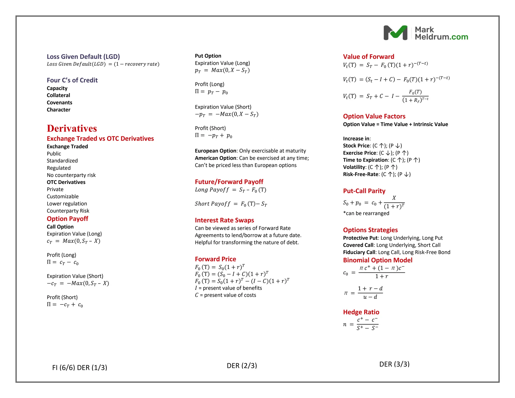
Expected Loss
𝐸𝑥𝑝𝑒𝑐𝑡𝑒𝑑 𝑙𝑜𝑠𝑠 = 𝐷𝑒𝑓𝑎𝑢𝑙𝑡 𝑝𝑟𝑜𝑏𝑎𝑏𝑖𝑙𝑖𝑡𝑦 × (1
− 𝑟𝑒𝑐𝑜𝑣𝑒𝑟𝑦 𝑟𝑎𝑡𝑒)
FI (3/6) FI (4/6) FI (5/6)
M.M140077214.

16. Loss Given Default (LGD)
𝐿𝑜𝑠𝑠 𝐺𝑖𝑣𝑒𝑛 𝐷𝑒𝑓𝑎𝑢𝑙𝑡(𝐿𝐺𝐷) = (1 − 𝑟𝑒𝑐𝑜𝑣𝑒𝑟𝑦 𝑟𝑎𝑡𝑒)
Four C’s of Credit
Capacity
Collateral
Covenants
Character
Derivatives
Exchange Traded vs OTC Derivatives
Exchange Traded
Public
Standardized
Regulated
No counterparty risk
OTC Derivatives
Private
Customizable
Lower regulation
Counterparty Risk
Option Payoff
Call Option
Expiration Value (Long)
𝑐𝑇 = 𝑀𝑎𝑥(0, 𝑆𝑇 – 𝑋)
Profit (Long)
Π = 𝑐𝑇 − 𝑐0
Expiration Value (Short)
−𝑐𝑇 = −𝑀𝑎𝑥(0, 𝑆𝑇 – 𝑋)
Profit (Short)
Π = −𝑐𝑇 + 𝑐0
Put Option
Expiration Value (Long)
𝑝𝑇 = 𝑀𝑎𝑥(0, 𝑋 − 𝑆𝑇)
Profit (Long)
Π = 𝑝𝑇 − 𝑝0
Expiration Value (Short)
−𝑝𝑇 = −𝑀𝑎𝑥(0, 𝑋 − 𝑆𝑇)
Profit (Short)
Π = −𝑝𝑇 + 𝑝0
European Option: Only exercisable at maturity
American Option: Can be exercised at any time;
Can’t be priced less than European options
Future/Forward Payoff
𝐿𝑜𝑛𝑔 𝑃𝑎𝑦𝑜𝑓𝑓 = 𝑆𝑇 – 𝐹0 (T)
𝑆ℎ𝑜𝑟𝑡 𝑃𝑎𝑦𝑜𝑓𝑓 = 𝐹0 (T)− 𝑆𝑇
Interest Rate Swaps
Can be viewed as series of Forward Rate
Agreements to lend/borrow at a future date.
Helpful for transforming the nature of debt.
Forward Price
𝐹0 (T) = 𝑆0(1 + 𝑟)𝑇
𝐹0 (T) = (𝑆0 − 𝐼 + 𝐶)(1 + 𝑟)𝑇
𝐹0 (T) = 𝑆0(1 + 𝑟)𝑇 − (𝐼 − 𝐶)(1 + 𝑟)𝑇
𝐼 = present value of benefits
𝐶 = present value of costs
Value of Forward
𝑉𝑡(T) = 𝑆𝑇 − 𝐹0 (T)(1 + 𝑟)−(𝑇−𝑡)
𝑉𝑡(T) = (𝑆𝑡 − 𝐼 + 𝐶) − 𝐹0(𝑇)(1 + 𝑟)−(𝑇−𝑡)
𝑉𝑡(T) = 𝑆𝑇 + 𝐶 − 𝐼 −
𝐹0(𝑇)
(1 + 𝑅𝐹)𝑇−𝑡
Option Value Factors
Option Value = Time Value + Intrinsic Value
Increase in:
Stock Price: (C ↑); (P ↓)
Exercise Price: (C ↓); (P ↑)
Time to Expiration: (C ↑); (P ↑)
Volatility: (C ↑); (P ↑)
Risk-Free-Rate: (C ↑); (P ↓)
Put-Call Parity
𝑆0 + 𝑝0 = 𝑐0 +
𝑋
(1 + 𝑟)𝑇
*can be rearranged
Options Strategies
Protective Put: Long Underlying, Long Put
Covered Call: Long Underlying, Short Call
Fiduciary Call: Long Call, Long Risk-Free Bond
Binomial Option Model
𝑐0 =
π𝑐+
+ (1 − π)𝑐−
1 + 𝑟
π =
1 + 𝑟 − 𝑑
𝑢 − 𝑑
Hedge Ratio
𝑛 =
𝑐+
− 𝑐−
𝑆+ − 𝑆−
FI (6/6) DER (1/3) DER (2/3) DER (3/3)
M.M140077214.

17. Alternative Investments
Hedge Funds
Equity Hedge: Market Neutral, Fundamental
Growth, Fundamental Value, Quantitative
Directional, Short Bias, Sector Specific
Event-Driven: Merger Arbitrage,
Distressed/Restructuring, Activist, Special Situations
Relative Value: FI Convertible Arbitrage, FI Asset
Backed, FI General, Volatility, Multi-Strategy
Macro
Fee Structure: Typically, 2 and 20; 2% of AUM and
20% of Profits
Private Equity
Leveraged Buyouts (LBOs): substantial use of
leverage to take companies private
LBO Target Characteristics: Strong and Sustainable
Cash Flows; Depressed Prices; Inefficient Companies
Venture Capital: Characterized by stage of company
of interest
1. Formative-stage financing: a) Angel Investing b)
Seed-Stage c) Early-Stage
2. Later-stage financing
3. Mezzanine-stage financing
Exit Strategies: Trade Sale, IPO, Recapitalization,
Secondary Sales, Write-Off/Liquidation
Valuation Methods: market or comparables,
discounted cash flow (DCF) and asset-based
Real Estate
Private Debt (Mortgages, Construction Lending)
Public Debt (MBS, CMOs)
Private Equity (Direct/Indirect Ownership)
Public Equity (REITs, Real Estate Development
Companies)
Valuation Approaches: Comparable Sales, Income,
Cost
Commodities
Precious Metals
Base Metals
Energy Products
Agricultural Products
Managed Futures: actively managed investment
funds
Futures price ≈ Spot price (1 + r) + Storage costs –
Convenience yield
Return Sources: Roll Yield, Collateral Yield, Changes
in Spot Price
Infrastructure
Long lived and capital intensive. These assets are
intended for public use, as they provide essential
services.
Fee Calculations
𝑀𝑎𝑛𝑎𝑔𝑒𝑚𝑒𝑛𝑡 𝐹𝑒𝑒 = 𝐴𝑠𝑠𝑒𝑡𝑠 𝑢𝑛𝑑𝑒𝑟 𝑚𝑎𝑛𝑎𝑔𝑒𝑚𝑒𝑛𝑡
× % 𝑀𝑎𝑛𝑎𝑔𝑒𝑚𝑒𝑛𝑡 𝑓𝑒𝑒
𝐼𝑛𝑐𝑒𝑛𝑡𝑖𝑣𝑒 𝐹𝑒𝑒 = 𝐺𝑎𝑖𝑛𝑠 𝑛𝑒𝑡 𝑜𝑓 𝑚𝑎𝑛𝑎𝑔𝑒𝑚𝑒𝑛𝑡 𝑓𝑒𝑒
× % 𝐼𝑛𝑐𝑒𝑛𝑡𝑖𝑣𝑒 𝑓𝑒𝑒
Hurdle Rate: Rate above which incentive fees are
paid. Hard hurdle rate: fess only apply to returns
that exceed the hurdle rate. Soft hurdle rate: fees
apply to the entire return.
High Water Mark: Highest cumulative return used
to calculate incentive fees
ALT (1/2) ALT (2/2)
M.M140077214.