This document analyzes the relationship between central bank interventions and exchange rate volatility. It decomposes exchange rate volatility into continuous and discontinuous (jump) components using bi-power variation. The analysis finds that while coordinated central bank interventions do not necessarily cause more jumps, the jumps that occur on intervention days tend to be larger. Coordinated interventions also predict the persistent, continuously varying component of volatility. By examining the timing and direction of jumps and interventions, the paper provides evidence that interventions normally generate jumps rather than reacting to them.
Developing economies are different than developed economies in many aspects, i.e., in terms of institutional framework and political situation etc. Thus, the monetary policy needed in developing countries is also different than developed countries. The goal of this study is to investigate exchange rate channel of monetary transmission mechanism in a developing country’s setup. The variables included in our analysis are interest rate, exchange rate, exports, consumer price index and gross domestic product. Johansen cointegration technique is applied to analyze the long run relationship among variables while multivariate VECM granger causality test is used to explore the direction of causality among the set of our variables. We use annual data ranging from 1980 to 2015 while taking account of the limitations of time series data. Our findings suggest that output has a negative long run relationship with exchange rate and interest rate, positive relationship with exports and no statistically significant relationship with inflation. Interest rate granger causes all four of our variables thus showing the power of this policy tool. Exchange rate causes exports, consumer price index and output which means exchange rate is the second most powerful variable in our analysis. Output is granger caused by interest rate, exports and exchange rate which confirms the sensitivity of output to these variables. Consumer price index is granger caused by all four of our variables and came out to be the most sensitive variable in our analysis.
In a recessionary and deflationary framework, the discretionary monetary policy cannot be optimal when the interest rate is already near zero and cannot decrease anymore. Indeed, when the Zero Lower Bound is binding, a negative demand shock implies a decrease in the current economic activity level and deflationary tensions, which cannot be avoided by monetary policy as the nominal interest rate can no longer decrease. The economic literature has then often recommended to target an inflation rate sufficiently above zero in order to avoid the dangers of this Zero Lower Bound (ZLB) constraint. On the contrary, provided the ZLB is not binding, monetary policy can efficiently contribute to the stabilization of economic activity and inflation in case of demand shocks. The variation in interest rates is then all the more accentuated as interest rate smoothing is a more negligible goal for the central bank. The contribution of our paper is to provide a clear analytical New-Keynesian framework sustaining these results. Besides, our analytical modelling also shows that even if the ZLB is currently not binding, the central bank should take into account the dangers of a potential future binding ZLB. Indeed, the interest rate should be decreased the fastest as a negative demand shock and the possibility to reach the ZLB is anticipated for a nearest future period. Our paper demonstrates the necessity of such a ‘pre-emptive’ active monetary policy even in a discretionary framework, which has the advantage to be time-consistent and to be in conformity with the empirical practices of independent central banks. We don’t have to make the strong hypothesis of a commitment monetary policy intended to affect private agents’ expectations in order to demonstrate the optimality of such a pre-emptive monetary policy.
Foreign Exchange Intervention and Currency Crisis (The Case of Korea During P...K Developedia
Title: Foreign exchange intervention and currency crisis
Sub Title: The case of Korea during pre-crisis period
Material Type: Report
Author: Kang, Sung-Kyung
Publisher: KDI School of Public Policy and Management
Date: 2000
Pages: 69
Subject Country: South Korea (Asia and Pacific)
Language: English
File Type: Documents
Original Format: pdf
Subject: Economy; Macroeconomics
Holding: KDI School of Public Policy and Management
The objective of this paper is to examine the impact of financial market development and liberalization on money demand behavior in Central African Economic and Monetary Community (CEMAC). We adopt the generalized method of moments (GMM) system for panel data. The empirical results indicate that financial liberalization has a negative impact on money demand. Moreover, real GDP and the GDP deflator affect it positively, while the main policy rate has a negative impact. In terms of economic policy involvement, monetary authorities must pursue reforms aimed at deepening financial liberalization measures so that banks actively participate in the financing of CEMAC economies.
Macroeconomic stability in the DRC: highlighting the role of exchange rate an...IJRTEMJOURNAL
This study is part of a macroeconomic approach and seeks to identify the role of the rate of
economic growth and the exchange rate in controlling the macroeconomic framework. The approaches adopted
in this paper are part of Keynesian thinking on macroeconomic stability using the macroeconomic stability
index proposed by Burnside and Dollars (2004) and A. Amine (2005). Our results argue that economic growth
is causing macroeconomic stability and that the exchange rate is negatively and significantly accounting for
macroeconomic stability in the Democratic Republic of Congo.
Analisis of housing bubble in USA, addresing from data panel model. Faculty of Economics and Centre for International Macroeconomics and Finance (CIMF).
University of Cambridge, Cambridge, CB3 9DD, UK
The Causal Analysis of the Relationship between Inflation and Output Gap in T...inventionjournals
The purpose of the paper is to study dynamic relationships between the inflation and output gap by using Granger causality, Impulse response and variance decompositions analysis within VECM framework for the quarterly data over the first period of 2003 and second period of 2016. The results of the study indicate that the output gap Granger cause the inflation in Turkey both in short-and long-runs. Also, sign of the causality is negative and same causal relationships between two variables hold beyond the sample period. The results should be taken as an evidence of the conclusion that the output gap has important implications for the CBRT's monetary policy.
The main purpose of this study is to examine if the International Fisher Effect holds between Mexico and the United States for the period from Q1: 2005 through Q3: 2016. The results of the test indicate a significant relationship between the interest rate differentials and the changes in the currency value between the two countries. The finding of this study is consistent with some of the earlier research while signifying the importance of other variables in improving the explanatory power of the independent variable.
Foundations of Financial Sector Mechanisms and Economic Growth in Emerging Ec...iosrjce
In this paper, we try to uncover the economic foundations of financial sector development and its
impacts on accelerating economic growth in the given context of emerging economies. We theorize and
empirically test a causally-motivated relationship among economic growth and related key financial sector
variables pertinent to this problem. We accomplish this by analyzing a 20 year panel-data constructed for 30
countries falling within the categorization of an ‘emerging economy’. We estimate the appropriate statistical
models along with related diagnostic tests. Finally, we comment on the strengths and weaknesses of our
approach and we try to explicate the economic rationale and justification for our formulation and the evidences
that follow
Despite a voluminous literature on the topic, the question of whether aid leads to growth is still controversial. To observe the pure effect of aid, researchers used instruments that must be exogenous to growth and explain well aid flows. This paper argues that instruments used in the past do not satisfy these conditions. We propose a new instrument based on predicted aid quantity and argue that it is a significant improvement relative to past approaches. We find a significant and relatively big effect of aid: a one standard deviation increase in received aid is associated with a 1.6 percentage points higher growth rate.
This study modeled volatility and daily exchange rate movement in Nigeria with daily exchange rate between Nigeria Naira and US Dollar from January 2, 2001 to May 20, 2019 collected from the Central Bank of Nigeria (CBN). The results of the estimated models revealed that conditional variance (volatility) has positive and significant relationship with exchange rate returns between Nigeria Naira and US Dollars, which corroborates the theory that predicts positive relationship between return and volatility for risk averse investors. Also found that exchange rate volatility between Naira / US Dollar is persistent. It was also discovered that goods news produces more volatility than bad news of equal magnitude. The researchers therefore suggested that the Central Bank of Nigeria should always proffer timely intervention to reduce the volatility persistence. This will go a long way to counteract or moderate the excess volatility between Naira and US Dollar transactions.
Abstract: The theoretical relationship of the long-run equilibrium between real exchange rates and interest rate differentials is essentially derived from the Purchasing Power Parity (PPP) and the uncovered interest parity. However, empirical evidence on this long-run relationship has rather been inconclusive. While several authors are able to establish the long-run relationship between real exchange rates and interest rate differentials other could not found this relationship. The reason for lack of relationship in some of the studies is as a result of omitted variables (Meese and Rogoff, 1988). Therefore, attempt is made in this study to evaluate this relationship between real exchange rate and interest rate differential for the case of Nigeria by controlling for foreign exchange reserves. The paper uses monthly data for the period 1993:1-2012:12 and applies Autoregressive Distributed Lags (ARDL) model. The estimates suggest the existence of long-run relationship between real exchange rate, interest rate differential and foreign exchange reserves. In the long run, the exchange rate coefficient has a positive effect on the foreign reserves. However, the effect of interest rate differential is negative and statistically significant. On the short run dynamics, the finding indicates a non-monotonic relationship between real exchange rate, interest rate differential and foreign exchange reserves. The out-of-sample forecast indicates a better forecast using ARMA model as all Theil coefficients are close zero for all the horizons used in the model.
The theoretical relationship of the long-run equilibrium between real exchange rates and interest rate differentials is essentially derived from the Purchasing Power Parity (PPP) and the uncovered interest parity. However, empirical evidence on this long-run relationship has rather been inconclusive. While several authors are able to establish the long-run relationship between real exchange rates and interest rate differentials other could not found this relationship. The reason for lack of relationship in some of the studies is as a result of omitted variables (Meese and Rogoff, 1988). Therefore, attempt is made in this study to evaluate this relationship between real exchange rate and interest rate differential for the case of Nigeria by controlling for foreign exchange reserves. The paper uses monthly data for the period 1993:1-2012:12 and applies Autoregressive Distributed Lags (ARDL) model. The estimates suggest the existence of long-run relationship between real exchange rate, interest rate differential and foreign exchange reserves. In the long run, the exchange rate coefficient has a positive effect on the foreign reserves. However, the effect of interest rate differential is negative and statistically significant. On the short run dynamics, the finding indicates a non-monotonic relationship between real exchange rate, interest rate differential and foreign exchange reserves. The out-of-sample forecast indicates a better forecast using ARMA model as all Theil coefficients are close zero for all the horizons used in the model.
Journal of Economic Literature 2011, 493, 652–672httpwww.a.docxtawnyataylor528
Journal of Economic Literature 2011, 49:3, 652–672
http:www.aeaweb.org/articles.php?doi=10.1257/jel.49.3.652
652
1. What’s International about
International Finance?
The exchange rate is an important asset price, perhaps the most important asset
price. It is also a distinctive asset price. The
price of Exxon stock or the ten-year Treasury
bond rate fluctuates over time in a reason-
ably consistent manner. By way of contrast,
the exchange rate has distinct, well-defined
regimes that are chosen by the government
and maintained by the central bank. No
entity essentially ever attempts to peg the
price of a stock or bond around a central par-
ity with narrow fluctuation bands.1 However,
some economies do fix their exchange rates
(for example, Denmark or Hong Kong),
while others do not (Canada, New Zealand).
A number of countries have changed their
minds on the topic and switched regimes
(Thailand in July 1997, Argentina in January
2002). Official authorities—at least some of
them—clearly reveal through their policies
1 I use “peg” and “fix” interchangeably.
Exchange Rate Regimes in the Modern
Era: Fixed, Floating, and Flaky
Andrew K. Rose*
This paper provides a selective survey of the incidence, causes, and consequences of a
country’s choice of its exchange rate regime. I begin with a critical review of Michael
Klein and Jay C. Shambaugh’s (2010) book Exchange Rate Regimes in the Modern Era,
and then proceed to provide an alternative overview of what the economics profession
knows and needs to know about exchange rate regimes. While a fixed exchange rate
with capital mobility is a well-defined monetary regime, floating is not; thus, it is
unclear whether it is theoretically sensible to compare countries across exchange rate
regimes. This comparison is quite difficult to make empirically. It is often hard to figure
out what the exchange rate regime of a country is in practice, since there are multiple
conflicting regime classifications. More importantly, similar countries choose radically
different exchange rate regimes without substantive consequences for macroeconomic
outcomes like output growth and inflation. That is, the profession knows surprisingly
little about either the causes or consequences of national choices of exchange rate
regimes. But since the consequences of these choices are small, understanding their
causes is of only academic interest. (JEL E52, F33)
* University of California, Berkeley, NBER, and CEPR.
I thank the Bank of England and INSEAD for hospitality;
Michael Klein, Jay Shambaugh, Alan Taylor, and the edi-
tor, Roger Gordon, for comments; and Jonathan Ostry for
sharing his work and data. The data set and key output are
freely available at http://faculty.haas.berkeley.edu/arose.
653Rose: Exchange Rate Regimes in the Modern Era
that they care about the exchange rate. One
would then like to understand both the
motivation and the consequences of these
decisions.
The fact ...
Exchange Rate Overshooting and its Impact on the Balance of Trade for the Tur...Hüseyin Tekler
Exchange rate overshooting is the short run phenomenon under the Dornbusch Model presented in 1976. We are really desiderative to find out whether the overshoots are for the short run or for the long run period for the Turkish economy. The estimated result using the Johansen Julius method and VECM, we have found that overshooting is for the short run period as opposed to the findings of Bahmani-Oskooee & Orhan (2000) while the Purchasing power parity [PPP] does not hold for the Turkish economy.
A study on the impact of global currency fluctuations with a special focus to...Aman Vij
The paper discusses about the factors influencing and impact of currency fluctuations on global economy. Then we shift our focus to Indian rupees factors which causes the Rupee fluctuations has been discussed. In the end we discuss about the steps taken by the RBI and the government and what else can be done by investors to lessen the impact of Global currency fluctuations and what can be done to prevent Indian Rupee fluctuation.
Empirical literature on money demand is mainly based on the estimation of a long run relation by means of time-invariant cointergration approach. Taiwan has experienced the economic and financial regime change since 1979. The purpose of this paper is to test structural breaks in Taiwan long run money demand equation. We examine six of the most influential specifications proposed in the literature. The classical set of explanatory variables (e.g. income and interest rates) is extended on the base of a number underlying economic reasons related to financial, labor and international portfolio characteristics. The results suggest that international financial market variables and the classical specifications are the key determinants of structural instability observed in Taiwan broad money.
Falcon stands out as a top-tier P2P Invoice Discounting platform in India, bridging esteemed blue-chip companies and eager investors. Our goal is to transform the investment landscape in India by establishing a comprehensive destination for borrowers and investors with diverse profiles and needs, all while minimizing risk. What sets Falcon apart is the elimination of intermediaries such as commercial banks and depository institutions, allowing investors to enjoy higher yields.
NO1 Uk Divorce problem uk all amil baba in karachi,lahore,pakistan talaq ka m...Amil Baba Dawood bangali
Contact with Dawood Bhai Just call on +92322-6382012 and we'll help you. We'll solve all your problems within 12 to 24 hours and with 101% guarantee and with astrology systematic. If you want to take any personal or professional advice then also you can call us on +92322-6382012 , ONLINE LOVE PROBLEM & Other all types of Daily Life Problem's.Then CALL or WHATSAPP us on +92322-6382012 and Get all these problems solutions here by Amil Baba DAWOOD BANGALI
#vashikaranspecialist #astrologer #palmistry #amliyaat #taweez #manpasandshadi #horoscope #spiritual #lovelife #lovespell #marriagespell#aamilbabainpakistan #amilbabainkarachi #powerfullblackmagicspell #kalajadumantarspecialist #realamilbaba #AmilbabainPakistan #astrologerincanada #astrologerindubai #lovespellsmaster #kalajaduspecialist #lovespellsthatwork #aamilbabainlahore#blackmagicformarriage #aamilbaba #kalajadu #kalailam #taweez #wazifaexpert #jadumantar #vashikaranspecialist #astrologer #palmistry #amliyaat #taweez #manpasandshadi #horoscope #spiritual #lovelife #lovespell #marriagespell#aamilbabainpakistan #amilbabainkarachi #powerfullblackmagicspell #kalajadumantarspecialist #realamilbaba #AmilbabainPakistan #astrologerincanada #astrologerindubai #lovespellsmaster #kalajaduspecialist #lovespellsthatwork #aamilbabainlahore #blackmagicforlove #blackmagicformarriage #aamilbaba #kalajadu #kalailam #taweez #wazifaexpert #jadumantar #vashikaranspecialist #astrologer #palmistry #amliyaat #taweez #manpasandshadi #horoscope #spiritual #lovelife #lovespell #marriagespell#aamilbabainpakistan #amilbabainkarachi #powerfullblackmagicspell #kalajadumantarspecialist #realamilbaba #AmilbabainPakistan #astrologerincanada #astrologerindubai #lovespellsmaster #kalajaduspecialist #lovespellsthatwork #aamilbabainlahore #Amilbabainuk #amilbabainspain #amilbabaindubai #Amilbabainnorway #amilbabainkrachi #amilbabainlahore #amilbabaingujranwalan #amilbabainislamabad
The secret way to sell pi coins effortlessly.DOT TECH
Well as we all know pi isn't launched yet. But you can still sell your pi coins effortlessly because some whales in China are interested in holding massive pi coins. And they are willing to pay good money for it. If you are interested in selling I will leave a contact for you. Just telegram this number below. I sold about 3000 pi coins to him and he paid me immediately.
Telegram: @Pi_vendor_247
The European Unemployment Puzzle: implications from population agingGRAPE
We study the link between the evolving age structure of the working population and unemployment. We build a large new Keynesian OLG model with a realistic age structure, labor market frictions, sticky prices, and aggregate shocks. Once calibrated to the European economy, we quantify the extent to which demographic changes over the last three decades have contributed to the decline of the unemployment rate. Our findings yield important implications for the future evolution of unemployment given the anticipated further aging of the working population in Europe. We also quantify the implications for optimal monetary policy: lowering inflation volatility becomes less costly in terms of GDP and unemployment volatility, which hints that optimal monetary policy may be more hawkish in an aging society. Finally, our results also propose a partial reversal of the European-US unemployment puzzle due to the fact that the share of young workers is expected to remain robust in the US.
USDA Loans in California: A Comprehensive Overview.pptxmarketing367770
USDA Loans in California: A Comprehensive Overview
If you're dreaming of owning a home in California's rural or suburban areas, a USDA loan might be the perfect solution. The U.S. Department of Agriculture (USDA) offers these loans to help low-to-moderate-income individuals and families achieve homeownership.
Key Features of USDA Loans:
Zero Down Payment: USDA loans require no down payment, making homeownership more accessible.
Competitive Interest Rates: These loans often come with lower interest rates compared to conventional loans.
Flexible Credit Requirements: USDA loans have more lenient credit score requirements, helping those with less-than-perfect credit.
Guaranteed Loan Program: The USDA guarantees a portion of the loan, reducing risk for lenders and expanding borrowing options.
Eligibility Criteria:
Location: The property must be located in a USDA-designated rural or suburban area. Many areas in California qualify.
Income Limits: Applicants must meet income guidelines, which vary by region and household size.
Primary Residence: The home must be used as the borrower's primary residence.
Application Process:
Find a USDA-Approved Lender: Not all lenders offer USDA loans, so it's essential to choose one approved by the USDA.
Pre-Qualification: Determine your eligibility and the amount you can borrow.
Property Search: Look for properties in eligible rural or suburban areas.
Loan Application: Submit your application, including financial and personal information.
Processing and Approval: The lender and USDA will review your application. If approved, you can proceed to closing.
USDA loans are an excellent option for those looking to buy a home in California's rural and suburban areas. With no down payment and flexible requirements, these loans make homeownership more attainable for many families. Explore your eligibility today and take the first step toward owning your dream home.
what is the best method to sell pi coins in 2024DOT TECH
The best way to sell your pi coins safely is trading with an exchange..but since pi is not launched in any exchange, and second option is through a VERIFIED pi merchant.
Who is a pi merchant?
A pi merchant is someone who buys pi coins from miners and pioneers and resell them to Investors looking forward to hold massive amounts before mainnet launch in 2026.
I will leave the telegram contact of my personal pi merchant to trade pi coins with.
@Pi_vendor_247
NO1 Uk Black Magic Specialist Expert In Sahiwal, Okara, Hafizabad, Mandi Bah...Amil Baba Dawood bangali
Contact with Dawood Bhai Just call on +92322-6382012 and we'll help you. We'll solve all your problems within 12 to 24 hours and with 101% guarantee and with astrology systematic. If you want to take any personal or professional advice then also you can call us on +92322-6382012 , ONLINE LOVE PROBLEM & Other all types of Daily Life Problem's.Then CALL or WHATSAPP us on +92322-6382012 and Get all these problems solutions here by Amil Baba DAWOOD BANGALI
#vashikaranspecialist #astrologer #palmistry #amliyaat #taweez #manpasandshadi #horoscope #spiritual #lovelife #lovespell #marriagespell#aamilbabainpakistan #amilbabainkarachi #powerfullblackmagicspell #kalajadumantarspecialist #realamilbaba #AmilbabainPakistan #astrologerincanada #astrologerindubai #lovespellsmaster #kalajaduspecialist #lovespellsthatwork #aamilbabainlahore#blackmagicformarriage #aamilbaba #kalajadu #kalailam #taweez #wazifaexpert #jadumantar #vashikaranspecialist #astrologer #palmistry #amliyaat #taweez #manpasandshadi #horoscope #spiritual #lovelife #lovespell #marriagespell#aamilbabainpakistan #amilbabainkarachi #powerfullblackmagicspell #kalajadumantarspecialist #realamilbaba #AmilbabainPakistan #astrologerincanada #astrologerindubai #lovespellsmaster #kalajaduspecialist #lovespellsthatwork #aamilbabainlahore #blackmagicforlove #blackmagicformarriage #aamilbaba #kalajadu #kalailam #taweez #wazifaexpert #jadumantar #vashikaranspecialist #astrologer #palmistry #amliyaat #taweez #manpasandshadi #horoscope #spiritual #lovelife #lovespell #marriagespell#aamilbabainpakistan #amilbabainkarachi #powerfullblackmagicspell #kalajadumantarspecialist #realamilbaba #AmilbabainPakistan #astrologerincanada #astrologerindubai #lovespellsmaster #kalajaduspecialist #lovespellsthatwork #aamilbabainlahore #Amilbabainuk #amilbabainspain #amilbabaindubai #Amilbabainnorway #amilbabainkrachi #amilbabainlahore #amilbabaingujranwalan #amilbabainislamabad
what is the future of Pi Network currency.DOT TECH
The future of the Pi cryptocurrency is uncertain, and its success will depend on several factors. Pi is a relatively new cryptocurrency that aims to be user-friendly and accessible to a wide audience. Here are a few key considerations for its future:
Message: @Pi_vendor_247 on telegram if u want to sell PI COINS.
1. Mainnet Launch: As of my last knowledge update in January 2022, Pi was still in the testnet phase. Its success will depend on a successful transition to a mainnet, where actual transactions can take place.
2. User Adoption: Pi's success will be closely tied to user adoption. The more users who join the network and actively participate, the stronger the ecosystem can become.
3. Utility and Use Cases: For a cryptocurrency to thrive, it must offer utility and practical use cases. The Pi team has talked about various applications, including peer-to-peer transactions, smart contracts, and more. The development and implementation of these features will be essential.
4. Regulatory Environment: The regulatory environment for cryptocurrencies is evolving globally. How Pi navigates and complies with regulations in various jurisdictions will significantly impact its future.
5. Technology Development: The Pi network must continue to develop and improve its technology, security, and scalability to compete with established cryptocurrencies.
6. Community Engagement: The Pi community plays a critical role in its future. Engaged users can help build trust and grow the network.
7. Monetization and Sustainability: The Pi team's monetization strategy, such as fees, partnerships, or other revenue sources, will affect its long-term sustainability.
It's essential to approach Pi or any new cryptocurrency with caution and conduct due diligence. Cryptocurrency investments involve risks, and potential rewards can be uncertain. The success and future of Pi will depend on the collective efforts of its team, community, and the broader cryptocurrency market dynamics. It's advisable to stay updated on Pi's development and follow any updates from the official Pi Network website or announcements from the team.
how to sell pi coins in South Korea profitably.DOT TECH
Yes. You can sell your pi network coins in South Korea or any other country, by finding a verified pi merchant
What is a verified pi merchant?
Since pi network is not launched yet on any exchange, the only way you can sell pi coins is by selling to a verified pi merchant, and this is because pi network is not launched yet on any exchange and no pre-sale or ico offerings Is done on pi.
Since there is no pre-sale, the only way exchanges can get pi is by buying from miners. So a pi merchant facilitates these transactions by acting as a bridge for both transactions.
How can i find a pi vendor/merchant?
Well for those who haven't traded with a pi merchant or who don't already have one. I will leave the telegram id of my personal pi merchant who i trade pi with.
Tele gram: @Pi_vendor_247
#pi #sell #nigeria #pinetwork #picoins #sellpi #Nigerian #tradepi #pinetworkcoins #sellmypi
Turin Startup Ecosystem 2024 - Ricerca sulle Startup e il Sistema dell'Innov...Quotidiano Piemontese
Turin Startup Ecosystem 2024
Una ricerca de il Club degli Investitori, in collaborazione con ToTeM Torino Tech Map e con il supporto della ESCP Business School e di Growth Capital
how to sell pi coins on Bitmart crypto exchangeDOT TECH
Yes. Pi network coins can be exchanged but not on bitmart exchange. Because pi network is still in the enclosed mainnet. The only way pioneers are able to trade pi coins is by reselling the pi coins to pi verified merchants.
A verified merchant is someone who buys pi network coins and resell it to exchanges looking forward to hold till mainnet launch.
I will leave the telegram contact of my personal pi merchant to trade with.
@Pi_vendor_247
Resume
• Real GDP growth slowed down due to problems with access to electricity caused by the destruction of manoeuvrable electricity generation by Russian drones and missiles.
• Exports and imports continued growing due to better logistics through the Ukrainian sea corridor and road. Polish farmers and drivers stopped blocking borders at the end of April.
• In April, both the Tax and Customs Services over-executed the revenue plan. Moreover, the NBU transferred twice the planned profit to the budget.
• The European side approved the Ukraine Plan, which the government adopted to determine indicators for the Ukraine Facility. That approval will allow Ukraine to receive a EUR 1.9 bn loan from the EU in May. At the same time, the EU provided Ukraine with a EUR 1.5 bn loan in April, as the government fulfilled five indicators under the Ukraine Plan.
• The USA has finally approved an aid package for Ukraine, which includes USD 7.8 bn of budget support; however, the conditions and timing of the assistance are still unknown.
• As in March, annual consumer inflation amounted to 3.2% yoy in April.
• At the April monetary policy meeting, the NBU again reduced the key policy rate from 14.5% to 13.5% per annum.
• Over the past four weeks, the hryvnia exchange rate has stabilized in the UAH 39-40 per USD range.
how can I sell pi coins after successfully completing KYCDOT TECH
Pi coins is not launched yet in any exchange 💱 this means it's not swappable, the current pi displaying on coin market cap is the iou version of pi. And you can learn all about that on my previous post.
RIGHT NOW THE ONLY WAY you can sell pi coins is through verified pi merchants. A pi merchant is someone who buys pi coins and resell them to exchanges and crypto whales. Looking forward to hold massive quantities of pi coins before the mainnet launch.
This is because pi network is not doing any pre-sale or ico offerings, the only way to get my coins is from buying from miners. So a merchant facilitates the transactions between the miners and these exchanges holding pi.
I and my friends has sold more than 6000 pi coins successfully with this method. I will be happy to share the contact of my personal pi merchant. The one i trade with, if you have your own merchant you can trade with them. For those who are new.
Message: @Pi_vendor_247 on telegram.
I wouldn't advise you selling all percentage of the pi coins. Leave at least a before so its a win win during open mainnet. Have a nice day pioneers ♥️
#kyc #mainnet #picoins #pi #sellpi #piwallet
#pinetwork
how to sell pi coins in all Africa Countries.DOT TECH
Yes. You can sell your pi network for other cryptocurrencies like Bitcoin, usdt , Ethereum and other currencies And this is done easily with the help from a pi merchant.
What is a pi merchant ?
Since pi is not launched yet in any exchange. The only way you can sell right now is through merchants.
A verified Pi merchant is someone who buys pi network coins from miners and resell them to investors looking forward to hold massive quantities of pi coins before mainnet launch in 2026.
I will leave the telegram contact of my personal pi merchant to trade with.
@Pi_vendor_247
Central Bank Intervention and Exchange Rate Volatility, Its Continuous and Jump Components
1. Research Division
Federal Reserve Bank of St. Louis
Working Paper Series
Central Bank Intervention and Exchange Rate Volatility,
Its Continuous and Jump Components
Michel Beine
Jérôme Lahaye
Sébastien Laurent
Christopher J. Neely
and
Franz C. Palm
Working Paper 2006-031C
http://research.stlouisfed.org/wp/2006/2006-031.pdf
May 2006
Revised February 2007
FEDERAL RESERVE BANK OF ST. LOUIS
Research Division
P.O. Box 442
St. Louis, MO 63166
______________________________________________________________________________________
The views expressed are those of the individual authors and do not necessarily reflect official positions of
the Federal Reserve Bank of St. Louis, the Federal Reserve System, or the Board of Governors.
Federal Reserve Bank of St. Louis Working Papers are preliminary materials circulated to stimulate
discussion and critical comment. References in publications to Federal Reserve Bank of St. Louis Working
Papers (other than an acknowledgment that the writer has had access to unpublished material) should be
cleared with the author or authors.
2. Central Bank Intervention and Exchange Rate Volatility, Its
Continuous and Jump Components∗
Michel BEINE†
Jérôme LAHAYE‡
Sébastien LAURENT§
Christopher J. NEELY¶
Franz C. PALMk
First version: May 2006
Revised: August 2006
This version: February 2007
Abstract
We analyze the relationship between interventions and volatility at daily and intra-daily
frequencies for the two major exchange rate markets. Using recent econometric methods to
estimate realized volatility, we employ bipower variation to decompose this volatility into a
continuously varying and jump component. Analysis of the timing and direction of jumps
and interventions imply that coordinated interventions tend to cause few, but large jumps.
Most coordinated operations explain, statistically, an increase in the persistent (continuous)
part of exchange rate volatility. This correlation is even stronger on days with jumps.
Keywords: Intervention, jumps, bi-power variation, exchange rate, volatility
JEL Codes: F31, F33, C34
∗The authors thank Mardi Dungey, Mark Taylor and participants at the International Journal of Finance
and Economics Conference on central bank intervention for very helpful comments and Justin Hauke for excellent
research assistance. This text presents research results of the Belgian Program on Interuniversity Poles of Attraction
initiated by the Belgian State, Prime Minister’s Office, Science Policy Programming. The scientific responsibility
is assumed by the authors. The views expressed are those of the individual authors and do not necessarily reflect
official positions of the Federal Reserve Bank of St. Louis, the Federal Reserve System, or the Board of Governors.
†University of Luxembourg and Free University of Brussels; mbeine@ulb.ac.be
‡CeReFiM, University of Namur and CORE; Jerome.Lahaye@fundp.ac.be
§CeReFiM, University of Namur and CORE; Sebastien.Laurent@fundp.ac.be
¶Assistant Vice President, Research Department, Federal Reserve Bank of St. Louis; neely@stls.frb.org
kMaastricht University, Faculty of Economics and Business Administration and CESifo; F.Palm@ke.unimaas.nl
1
3. 1 Introduction
During a period of twenty years (1985-2004), the central banks of the U.S., Japan and Germany
(Europe) intervened more than 600 times in either the DEM-dollar (DEM/USD or EUR/USD after
the introduction of the euro) or the yen-dollar (JPY/USD) market. On average, they intervened
almost three times per month. It is not surprising that central banks should frequently intervene
in markets that are of crucial importance for international competitiveness. Given the importance
of understanding foreign exchange markets, for scientific and policy reasons, one would like to
assess the impact of central bank interventions (CBIs hereafter) on exchange rates.
The large empirical literature on the impact of CBIs provides mixed evidence on the impact
of CBI on exchange rate returns. In general, authors fail to identify effects on the conditional
mean of exchange rate returns at a daily frequency (Baillie and Osterberg 1997). When effects on
the spot exchange rate returns are detected, they are often found to be perverse, i.e. purchases
of U.S. dollar leading to a depreciation of the dollar (Baillie and Osterberg 1997, Beine, Bénassy-
Quéré, and Lecourt 2002). This perverse result tends to hold for both unilateral and coordinated
interventions. This result has usually been interpreted as indicating a lack of credibility, or ascribed
to inappropriate identification schemes in the presence of leaning-against-the-wind policies (Neely
2005b). Recent studies conducted at intra-daily frequencies nevertheless find that CBIs can move
the exchange rate, at least in the very short run (Fischer and Zurlinden 1999, Dominguez 2003).
The empirical literature is much more conclusive with respect to the impact of CBIs in terms
of exchange rate volatility. Most studies conclude that intervention tends to increase exchange
rate volatility (Humpage 2003) and this result is robust to the use of any of the three main mea-
sures of asset price volatility: univariate GARCH models (Baillie and Osterberg 1997, Dominguez
1998, Beine, Bénassy-Quéré, and Lecourt 2002); implied volatilities extracted from option prices
(Bonser-Neal and Tanner 1996, Dominguez 1998, Galati and Melick 1999); and realized volatility
(Beine, Laurent, and Palm 2005, Dominguez 2004).
This paper looks at the relation between intervention and the components of volatility. We in-
vestigate how CBIs affect the continuous, persistent part of exchange rate volatility and the discon-
tinuous component. Our approach relies on bi-power variation (Barndorff-Nielsen and Shephard
(2004, 2006)) to decompose exchange rate changes into a continuous part and a jump compo-
nent. Bi-power variation consistently estimates the continuous volatility even in the presence of
jumps (i.e. for a continuous-time jump diffusion process). And the realized volatility (sum of
2
4. squared intradaily returns) consistently estimates the sum of both the continuous volatility and
the discontinuities (jumps) in the underlying price process. Therefore the difference between real-
ized volatility and the bi-power variation consistently estimates the contribution to the quadratic
variation process due to the discontinuities (jumps).
Barndorff-Nielsen and Shephard (2006) suggest that jumps in foreign exchange markets are
linked to the arrival of macroeconomic news, in line with the results of Andersen, Bollerslev,
Diebold, and Vega (2003). In this respect, our findings illuminate the importance of interventions
for explaining the dynamics of exchange rates and the extent to which interventions impact rates
similarly to macroeconomic news.
Our investigation covers central bank activity on the two largest exchange rate markets. We
focus on Fed, Bundesbank (ECB after 1998) and Bank of Japan interventions over the last twenty
years. Using the method of bi-power variation with 5-minute exchange rate data, we identify the
days in which exchange rates jumps occur. This allows us to investigate whether intervention days
are associated with the occurrence of these jumps.
To achieve this goal, we proceed in five steps.
First, we decompose realized volatility into a continuous component and a jump component.
We investigate the relationship between CBIs and discontinuities in the JPY/USD and USD/EUR
markets and find that while jumps are not more likely to occur on days of intervention, the
jumps that do occur are larger than average. In particular, only a few coordinated interventions
could reasonably generate jumps. Coordinated CBIs do predict the smooth, persistently varying
component of realized volatility, however.
Second, to check for the direction of causality between jumps and coordinated CBIs, we care-
fully study the number of jumps and the timing of their occurrence during the CBI days. Most
of the jumps on CBI days occurred during or after the overlap of European and U.S. markets,
when most coordinated interventions take place. We then examine the direction of the jumps and
coordinated CBIs for days on which they both occur. This analysis strongly suggests that inter-
vention normally generates the jumps, rather than reacting to them. The only period in which
intervention appears to respond to jumps is that of the ”Louvre Accords,” when central banks
were very keen to dampen volatility by leaning against the wind.
Third, to control for the impact of macroeconomic announcements on exchange rate volatility,
we check for the joint occurrence of jumps, coordinated interventions on the corresponding for-
eign exchange markets and of macroeconomic announcements. For the JPY/USD, macroeconomic
3
5. announcements were made on half of the 14 days where jumps occurred and a coordinated in-
tervention took place in this market. For the USD/EUR market, macroeconomic announcements
occurred only on three out of 10 days with jumps in the exchange rate and a coordinated inter-
vention. The timing evidence suggests that a subset of jumps on these days were not the result
of macroeconomic announcements. Instead, some coordinated interventions might be the primary
cause of the observed discontinuities.
Fourth, a formal regression analysis confirms these findings.
Fifth, we discuss the economic interpretation of the findings, the implications for foreign ex-
change market policy of central banks and some extensions of the methodology.
The paper is organized as follows. Section 2 details the procedure used to identify the jump
components of the realized volatilities. Section 3 provides some details on the data. Section 4
reports our empirical analysis relating the occurrence of jumps with CBIs while Section 5 proposes
an interpretation of the main findings. Finally, Section 6 concludes.
2 Extracting the jump component
Let p(t) be a logarithmic asset price at time t. Consider the continuous-time jump diffusion process
dp(t) = µ(t)dt + σ(t)dW(t) + κ(t)dq(t), 0 ≤ t ≤ T, (1)
where µ(t) is a continuous and locally bounded variation process, σ(t) is a strictly positive
stochastic volatility process with a sample path that is right continuous and has well defined
limits, W(t) is a standard Brownian motion, and q(t) is a counting process with intensity λ(t)
(P[dq(t) = 1] = λ(t)dt and κ(t) = p(t) − p(t−) is the size of the jump in question). The quadratic
variation for the cumulative process r(t) ≡ p(t)−p(0) is the integrated volatility of the continuous
sample path component plus the sum of the q(t) squared jumps that occurred between time 0 and
time t:
[r, r]t =
Z t
0
σ2
(s)ds +
X
0<s≤t
κ2
(s). (2)
Now, let us define the daily realized volatility as the sum of the corresponding intradaily
squared returns:
RVt+1(∆) ≡
1/∆
X
j=1
r2
t+j∆,∆, (3)
4
6. where rt,∆ ≡ p(t) − p(t − ∆) is the discretely sampled ∆-period return.1
So 1/∆ is the number of
intradaily periods (288 in our application).
In order to disentangle the continuous and the jump components of realized volatility, we need
to consistently estimate integrated volatility, even in the presence of jumps in the process. This
is done using the asymptotic results of Barndorff-Nielsen and Shephard (2004, 2006).
Barndorff-Nielsen and Shephard (2004) show that the realized volatility converges uniformly
in probability to the increment of the quadratic variation process as the sampling frequency of the
returns increases (∆ → 0):2
RVt+1(∆) →
Z t+1
t
σ2
(s)ds +
X
t<s≤t+1
κ2
(s). (4)
That means that realized volatility consistently estimates integrated volatility as long as there
are no jumps. The realized bi-power variation is defined as the sum of the product of adjacent
absolute intradaily returns standardized by a constant:
BVt+1(∆) ≡ µ−2
1
1/∆
X
j=2
|rt+j∆,∆||rt+(j−1)∆,∆|, (5)
where µ1 ≡
p
2/π ' 0.79788 is the mean of the absolute value of a standard normally distributed
random variable. It can indeed be shown that even in the presence of jumps,
BVt+1(∆) →
Z t+1
t
σ2
(s)ds. (6)
Thus, the difference between the realized volatility and the bi-power variation consistently
estimates the jump contribution to the quadratic variation process. When ∆ → 0:
RVt+1(∆) − BVt+1(∆) →
X
t<s≤t+1
κ2
(s). (7)
Moreover, because a finite sample estimate of the squared jump process might be negative (in
Equation (7)), we truncate the measurement at zero, i.e.
Jt+1(∆) ≡ max[RVt+1(∆) − BVt+1(∆), 0]. (8)
One might wish to select only statistically significant jumps, to consider very small jumps to
be part of the continuous sample path rather than genuine discontinuities. The Barndorff-Nielsen
1We use the same notation as in Andersen, Bollerslev, and Diebold (2005) and normalize the daily time interval
to unity. We drop the ∆ subscript for daily returns: rt+1,1 ≡ rt+1.
2See also, for example, Andersen and Bollerslev (1998a), Andersen, Bollerslev, Diebold, and Labys (2001),
Barndorff-Nielsen and Shephard (2002a), Barndorff-Nielsen and Shephard (2002b), Comte and Renault (1998).
5
7. and Shephard (2004, 2006) results, extended in Barndorff-Nielsen, Graversen, Jacod, Podolskij,
and Shephard (2005), imply:3
RVt+1(∆) − BVt+1(∆)
q
(µ−4
1 + 2µ−2
1 − 5)∆
R t+1
t
σ4(s)ds
→ N(0, 1), (9)
when there is no jump and for ∆ → 0, under sufficient regularity conditions. We need to estimate
the integrated quarticity
R t+1
t
σ4
(s)ds to compute this statistic. The realized tri-power quarticity
measure permits us to estimate it consistently, even in the presence of jumps:
TQt+1(∆) ≡ ∆−1
µ−3
4/3
1/∆
X
j=3
|rt+j∆,∆|4/3
|rt+(j−1)∆,∆|4/3
|rt+(j−2)∆,∆|4/3
, (10)
with µ4/3 ≡ 22/3
Γ(7/6)Γ(1/2)−1
. Thus, we have that, for ∆ → 0:
TQt+1(∆) →
Z t+1
t
σ4
(s)ds. (11)
The implementable statistic is therefore:
Wt+1(∆) ≡
RVt+1(∆) − BVt+1(∆)
q
∆(µ−4
1 + 2µ−2
1 − 5)TQt+1(∆)
. (12)
However, following Huang and Tauchen (2005) and Andersen, Bollerslev, and Diebold (2005),
we actually implement the following statistic:
Zt+1(∆) ≡ ∆−1/2 [RVt+1(∆)) − BVt+1(∆)]RVt+1(∆)−1
[(µ−4
1 + 2µ−2
1 − 5)max{1, TQt+1(∆)BVt+1(∆)−2}]1/2
. (13)
Huang and Tauchen (2005) show that the statistic defined in Equation (12) tends to over-reject
the null hypothesis of no jumps. Moreover, they show that Zt+1(∆) defined in Equation (13) is
closely approximated by a standard normal distribution and has reasonable power against several
plausible stochastic volatility jump diffusion models. Practically, we choose a significance level α
and compute:
Jt+1,α(∆) = I[Zt+1(∆) > Φα] · [RVt+1(∆) − BVt+1(∆)], (14)
3Note that these results rely on the assumption that the joint process of the drift and volatility of the underlying
process (µ, σ) is independent of the Brownian motion W. This rules out leverage effects and feedback between
previous innovations in W and the risk premium in µ. This is empirically reasonable for foreign exchange markets,
but not for equity data.
6
8. where Φα is the critical value associated with α. Of course, a smaller α means that we estimated
fewer and larger jumps. Moreover, to make sure that the sum of the jump component and the
continuous one equals realized volatility, we impose:
Ct+1,α(∆) = I[Zt+1(∆) ≤ Φα] · RVt+1(∆) + I[Zt+1(∆) > Φα] · BVt+1(∆). (15)
Finally, still following Andersen, Bollerslev, and Diebold (2005), we use a modified staggered
realized bi-power variation and tri-power quarticity measure to tackle first order autocorrelation
due to microstructure noise issues:4
BVt+1(∆) ≡ µ−2
1 (1 − 2∆)−1
1/∆
X
j=3
|rt+j∆,∆||rt+(j−2)∆,∆|, (16)
TQt+1(∆) ≡ ∆−1
µ−3
4/3(1 − 4∆)−1
1/∆
X
j=5
|rt+j∆,∆|4/3
|rt+(j−2)∆,∆|4/3
|rt+(j−4)∆,∆|4/3
. (17)
Barndorff-Nielsen and Shephard (2004) show that in the absence of microstructure noise, the
asymptotic distribution of the test statistic defined in Equation (13) remains asymptotically stan-
dard normal once the relevant components are replaced by the staggered ones.
3 Data
3.1 Exchange rate data
We analyze the interaction between jumps and interventions for the two major exchange rate
markets, namely the Japanese Yen (JPY) and the Deutsche Mark (DEM) (Euro after 1998) against
the US Dollar (USD). For these two exchange rates, we have about 17 years of intradaily data for
a period ranging from January 2, 1987 to October 1, 2004, provided by Olsen and Associates. The
raw data consists of last mid-quotes (average of the logarithms of bid and ask quotes) of 5-minute
intervals throughout the global 24-hour trading day. We obtain 5-min returns as 100 times the
first difference of the logarithmic prices.
Following Andersen and Bollerslev (1998b), one trading day extends from 21.00 GMT on day
t − 1 to 21.00 GMT on date t. This definition ensures that all interventions dated at day t (using
local time) take place during this interval, even the Japanese interventions that may occur before
00.00 GMT.
4Considering first-order autocorrelation is sufficient in our application.
7
9. It is important to get rid of the trading days that display either too many missing values or
low trading activity. To this aim, we delete week-ends plus a set of fixed and irregular holidays.5
Moreover we use three additional criteria. First, we do not consider the trading days for which
there are more than 100 missing values at the 5-minute frequency. Second, days where we record
more than 50 zero intra-daily returns are deleted. Finally, we suppress days for which more than
7 consecutive prices were found to be the same. Using these criteria leads us to suppress 48 and
85 days, respectively, for the USD/EUR and the JPY/USD.
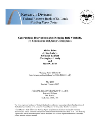
Figures 1 and 2 plot the evolution of the exchange rate and the return at a daily frequency
over the whole sample for the USD/EUR and the JPY/USD.6
Figures 3 and 4 plot the evolution of the three main measures of volatility: the realized
volatility built from the 5-minute intradaily returns (first panel), as described in Equation (3),
and its decomposition into the continuous sample path (second panel) and the jump component
(third panel), as described, respectively, in equations (15) and (14). The significance of the jump
component was assessed using a conservative 99.99 % confidence level, i.e. α = 0.9999.
Tables 1 and 2 describe the realized volatility estimates as well as the estimated jump com-
ponents for the USD/EUR and JPY/USD series. These tables also report the proportion of
significant values over the whole sample. Two significance levels are used. We use first a very low
level (α = 0.5, variable denoted J in the table) for which at least one jump is detected almost
every day: the proportion of days with jumps is above 90% for both markets. The use of such
a significance level would of course result in an overestimation of the number of economically
meaningful jumps. Therefore, we use a much more conservative significance level (α = 0.9999,
variable denoted J9999 in the table) for which the proportion of days with jumps is much lower
(about 10 to 13% of the business days).7
5Fixed holidays include Christmas (December 24 - 26), New Year (December 31 - January 2), and July Fourth.
Moving holidays include Good Friday, Easter Monday, Memorial Day, Labor Day, Thanksgiving and the day after,
and July Fourth when it falls officially on July 3.
6The two figures are drawn using the filtered data. This means that some business days where the activity
and/or the data quality is low were suppressed. We thus implicitly assume that during these removed days, the
exchange rate did not change.
7While the choice of α (0.9999) for our main results is consistent with the literature, we have investigated how
changing α affects the probability of intervention, conditional on a jump, and found that the inference was not very
sensitive to the choice of α.
8
10. 0.8
0.9
1
1.1
1.2
1.3
1.4
1.5
1986 1988 1990 1992 1994 1996 1998 2000 2002 2004 2006
Price
Days
Daily Price
-4
-3
-2
-1
0
1
2
3
4
1986 1988 1990 1992 1994 1996 1998 2000 2002 2004 2006
Return
Days
Daily Return
Figure 1: Dollar/Euro - Daily prices and daily returns
80
90
100
110
120
130
140
150
160
1986 1988 1990 1992 1994 1996 1998 2000 2002 2004 2006
Price
Days
Daily Price
-8
-6
-4
-2
0
2
4
6
1986 1988 1990 1992 1994 1996 1998 2000 2002 2004 2006
Return
Days
Daily Return
Figure 2: JPY/Dollar - Daily prices and daily returns
3.2 Intervention data
This paper uses official data on U.S., German (ECB after 1998) and Japanese interventions pro-
vided by those central banks. The investigation period is similar to sample period for the exchange
9
11. 0
2
4
6
8
10
12
1986 1988 1990 1992 1994 1996 1998 2000 2002 2004 2006
RV
Days
Realized Volatility
0
1
2
3
4
5
6
1986 1988 1990 1992 1994 1996 1998 2000 2002 2004 2006
Cont.Comp.
Days
Continuous Component - alpha = 0.9999
0
1
2
3
4
5
6
7
8
1986 1988 1990 1992 1994 1996 1998 2000 2002 2004 2006
Jump
Days
Jump - alpha = 0.9999
Figure 3: Dollar/Euro - Daily RV, continuous component and jumps
0
5
10
15
20
25
30
35
1986 1988 1990 1992 1994 1996 1998 2000 2002 2004 2006
RV
Days
Realized Volatility
0
5
10
15
20
25
30
35
1986 1988 1990 1992 1994 1996 1998 2000 2002 2004 2006
Cont.Comp.
Days
Continuous Component - alpha = 0.9999
0
0.5
1
1.5
2
2.5
3
1986 1988 1990 1992 1994 1996 1998 2000 2002 2004 2006
Jump
Days
Jump - alpha = 0.9999
Figure 4: JPY/Dollar - Daily RV, continuous component and jumps
rate data (January 1987-October 2004). While official data for the Fed and the Bundesbank are
available at the daily frequency for the whole sample, official data for the Bank of Japan are avail-
10
12. RV log(RV ) J J9999
Prop. - - 0.9069 0.1034
Obs. 4360. 4360. 4360. 4360.
Mean 0.5577 -0.7727 0.07115 0.02575
St. Dev. 0.4593 0.5819 0.1761 0.1696
Skew. 5999 0.4120 19.47 22.21
Kurt. 82.48 3999 638.8 763.5
Min. 0.06499 -2734 0.0000 0.0000
Max. 10.92 2391 7109 7.109
LB(8) 3942. 8476. 55.76 4.173
Table 1: Descriptive statistics on the USD/EUR. Descriptive statistics for realized volatility (RV ), log
realized volatility (log(RV )), jumps (J, α = 0.5), and significant jumps (J9999, α = 0.9999). The rows are: propor-
tion of jumps in the sample, number of observation, mean, standard deviation, skewness, kurtosis, minimum of the
sample and maximum. We also provide the Ljung Box statistic LB with 8 lags (the number of lags = log(obs)).
For a size of 5%, the critical value for the LB test with 8 degrees of freedom is 15.51.
RV log(RV ) J J9999
Prop. - - 0.9424 0.1339
Obs. 4360. 4360. 4360. 4360.
Mean 0.6433 -0.6955 0.08284 0.02670
St. Dev. 0.7730 0.6636 0.1295 0.1081
Skew. 19.32 0.4597 6621 9.410
Kurt. 727.0 3964 77.92 146.0
Min. 0.04106 -3193 0.0000 0.0000
Max. 33.03 3497 2511 2.511
LB(8) 4066. 10920000 1337. 11.19
Table 2: Descriptive statistics on the JPY/USD. Descriptive statistics for realized volatility (RV ), log
realized volatility (log(RV )), jumps (J, α = 0.5), and significant jumps (J9999, α = 0.9999). The rows are: propor-
tion of jumps in the sample, number of observation, mean, standard deviation, skewness, kurtosis, minimum of the
sample and maximum. We also provide the Ljung Box statistic LB with 8 lags (the number of lags = log(obs)).
For a size of 5%, the critical value for the LB test with 8 degrees of freedom is 15.51.
11
13. able only after April 1991. As a result, we complement the official data set with days of perceived
BoJ intervention. The perceived intervention days are those for which there was at least one
report of intervention in financial newspapers (Wall Street Journal and Financial Times). While
this might result in some misestimation of intervention, this procedure allows us to have similar
samples of data for the two exchange rate markets and makes the comparison easier.
Table 3 reports the number of intervention days for the two FX markets. We distinguish
between coordinated and unilateral interventions. Interventions are considered coordinated when
both central banks intervened in the same market on the same day and in the same direction.
Both theoretical and empirical rationales motivate such a distinction. Coordinated interventions
are supposed to affect the market differently than unilateral operations, as the joint presence of
the central banks sends a much more powerful signal to market participants. This conjecture is
supported by empirical studies by Catte, Galli, and Rebecchini (1992) and Beine, Laurent, and
Palm (2005) which show that the response of the exchange rate to interventions is much stronger
for coordinated operations.
USD/EUR JPY/USD
Coord. 111 115
FED 83 48
Bundesbank 97 -
BoJ - 343
Table 3: Number of Official intervention days from January 2, 1987 to October 31, 2004. The Table
reports the number of official intervention days for the Federal Reserve (FED), the Bundesbank and the Bank of
Japan (BoJ). For the Bank of Japan, data before April 1, 1991 are interventions reported in the Wall Street Journal
and/or the Financial Times.
4 Results
4.1 Jumps and CBIs at the daily frequency
As a first step to analyze the impact of CBIs on the two components of realized volatility, one can
look at how often statistically significant jumps occur on days of interventions. At this stage, we
ignore the question of causality between exchange rate dynamics and interventions (Neely 2005b)
12
14. and simply look at the proportion of intervention days for which jumps are detected. We will
confront the issue of causality between jumps and interventions later on, through a closer inspection
of the intra-daily patterns of these jumps.
Table 4 provides some descriptive statistics for the significant jump components extracted on
the non-intervention days on the USD/EUR market (first panel) and JPY/USD market (second
panel) and on the intervention days. The three parts of the table correspond respectively to
days without CBIs (labeled ‘No CBIs’), with a unilateral or coordinated intervention (labeled
‘CBIs of any type’) and finally days associated with a coordinated intervention of the two involved
central banks (labeled ‘Coordinated Interventions’). Each part of the table contains three columns
corresponding to the significant jumps (J9999), continuous volatility (CC9999) and significant
jumps conditional on a jump day, or in other words non-zero jumps (J9999 > 0). In each case,
we chose α = 0.9999.
Two main results emerge from these tables. First, one cannot reject that the likelihood of
a jump is independent of intervention. This result holds both for all intervention days and for
the days in which concerted operations took place. For instance, the proportion of days with
significant jumps when a coordinated intervention was conducted by the Fed and the Bundesbank
(or the ECB) on the USD/EUR market is slightly lower (0.094) than the one observed on the
non-intervention days (0.104). This suggests that if interventions affect exchange rate volatility,
they are not associated with an abnormal probability of jumps. Second, while the proportion
of jumps on the intervention days is not significantly higher, jumps are bigger when there is an
intervention. This is obviously the case for the USD/EUR. The ratios of the size of jumps between
intervention days and non-intervention days are 2.52 and 4.92, for all types of operations and con-
certed interventions, respectively. Therefore, while one cannot obviously claim that interventions
systematically create jumps on exchange rates, a subset of these interventions is associated with
large discontinuities in exchange rates. Because the evidence that coordinated intervention is as-
sociated with unusually large jumps is stronger than that for unilateral operations, the subsequent
analysis will focus on such concerted operations.
4.2 Jumps and CBIs: some further causality analysis
The previous results suggest that several jumps occurred, on average, on the day of a coordinated
intervention.
Table 4 identifies 10 and 14 coordinated interventions days for which at least one significant
13
16. jump was detected at the 0.01% level in the USD/EUR and the JPY/USD markets, respectively.
Such preliminary evidence does not imply that those interventions created the jumps in the FX
markets, however, for two reasons.
The first reason is related to reverse causality. As emphasized by recent contributions in the
literature (Kearns and Rigobon 2004, Neely 2005a, Neely 2005b), interventions are not conducted
in a random way and tend to react rather to exchange rate developments. This implies that
statistical analysis of interventions should devote special attention to determining the direction
of causality. As pointed out by Neely (2005b), this is particularly important to account for when
conducting the investigation at the daily frequency.
The second reason why causal links between interventions and jumps might be spurious is the
presence of macroeconomic announcements. These macro announcements are known to create
jumps in the FX markets (Andersen, Bollerslev, Diebold, and Vega 2003). Therefore, it is impor-
tant to check for the presence of such announcements on the investigated intervention days.
Jumps and CBIs: intra-daily investigation
One way to investigate the direction of the causality between jumps and interventions is to
look at the intra-daily patterns of these events.
Unfortunately, one cannot obtain the precise times of intervention because such times were not
recorded by the trading desks of most major central banks. Auxiliary information permits this
unavailability to be overcome. One could use the timing of newswire reports of those operations,
as proposed by Dominguez (2004) for Fed interventions. While potentially useful, this approach
presents drawback in that it is unclear whether the timing of the reports is consistent with that
of the actual operations. Using real-time data of the interventions of the Swiss National Bank,
Fischer (2005) shows that significant discrepancies in terms of timings emerge between Reuters
reports of the interventions and the actual operations of the Swiss monetary authorities. Some of
these differences are expressed in hours rather than in minutes.
An alternative approach to the use of newswire reports is to start from the stylized fact that
most of the central banks tend to operate within the predominant business hours of their countries
(Neely 2000). An investigation of the empirical distributions of the reported timings of the Fed,
the Bundesbank and the BoJ interventions corroborates this stylized fact (Dominguez 2004). Fur-
thermore, European and U.S. monetary authorities reportedly tend to intervene in concert during
the overlap of European and U.S. markets to maximize the signalling content of these operations.
15
17. This stylized fact is supported by the timing of Reuters news collected over the 1989-1995 pe-
riod.8
Although the timing of the Reuters reports should be treated cautiously, most coordinated
intervention headlines fall within the overlap of the markets, suggesting that the assumption that
coordinated interventions occur in the afternoon European time is reasonable. This means that,
at least for the USD/EUR market, the timing of these jumps can be compared to this time range.
Jumps occurring before the overlap period probably cannot be ascribed to coordinated interven-
tions. Instead, such jumps might motivate intervention. But, intervention might well cause the
discontinuities observed during the overlap.
Intra-daily timing of jumps
We first assume that coordinated interventions occur during the trading overlap of financial
markets in Europe and the United States. To get a precise time for the jumps, we find the
maximum intra-daily absolute exchange rate return. For both exchange rates (USD/EUR and
JPY/USD), we focus on days on which there was both intervention and a discontinuity in the
exchange rate. Panel 1 of Figure 5 reports the distribution of the time interval with the high-
est intra-daily return for all the intervention days (coordinated or unilateral interventions) in the
USD/EUR, while Panel 2 gives the same information but only for days of coordination interven-
tions.
Panel 2 of Figure 5 shows that for 7 out of 10 events, the maximum intra-daily exchange
rate return falls within the short overlap period of U.S. and European markets. Therefore, for
those 7 coordinated intervention episodes, coordinated operations might have created the jumps.
Of course, other events, like macro announcements, also might have created the discontinuities.
Panel 1 of Figure 5, however, also includes days of unilateral interventions. In the case of unilateral
operations, the central banks can intervene over the full course of the day because there is no need
to coordinate. Interestingly, the discontinuities were much more dispersed on the days of unilateral
intervention. This pattern, that jumps are more concentrated on days of coordinated interventions,
is consistent with the idea that intervention is related to the jumps.
The same investigation might also be conducted for the interventions days on the JPY/USD
market. The lack of overlap between U.S. and Japanese markets leaves the likely timing of coor-
dinated intervention ambiguous, however. Nevertheless, for the sake of completeness, we provide
8Olsen and Associates provided Reuters headlines for the days of G-3 intervention from 1989 to 1995. Dominguez
(2002) previously used these data for intraday analysis.
16
18. 0 12 24 36 48 60 72 84 96 108 120 132 144 156 168 180 192 204 216 228 240 252 264 276 288
0
1
2
3
4
Time occurrence of the maximum intra−day return − days of CBI (coordinated or unilateral)
Intra−Day Periods
Count
of
Maximum
Returns
Tokyo opening
(0.00 GMT) Tokyo lunch
starts
(3.00 GMT)
Tokyo lunch
ends
(4.30 GMT)
European segment
opening
(6.00 GMT)
North american
segment opening
(12.00 GMT)
European segment
ends
(15.00 GMT)
0 12 24 36 48 60 72 84 96 108 120 132 144 156 168 180 192 204 216 228 240 252 264 276 288
0
1
2
3
4 Time occurrence of the maximum intra−day return − days of coordinated CBI
Intra−Day Periods
Count
of
Maximum
Returns
Tokyo opening
(0.00 GMT) Tokyo lunch
starts
(3.00 GMT)
Tokyo lunch
ends
(4.30 GMT)
European segment
opening
(6.00 GMT)
North american
segment opening
(12.00 GMT)
European segment
ends
(15.00 GMT)
Figure 5: USD/EUR - Fed and BB intervention days (Panel 1: coordinated or unilat-
eral. Panel 2: coordinated) where a jump occurred. Count of daily maximum intra-day
returns per intra-day periods. The graph shows, for each intra-day period, how many days have
their maximum intra-day return at the intra-day interval in question.
the corresponding figures for the all-type intervention days as well as the days of coordinated
interventions (see Figure 6).
The previous informal timing evidence can be complemented by a more robust statistical
analysis of the intra-daily pattern of the exchange rate returns. The previous analysis neglects
the fact that more than one jump can occur on a particular day. For instance, a second jump on
the USD/EUR might occur during the overlap period, restoring the possibility that coordinated
operations between the Fed and Bundesbank create this jump. Therefore, it is possible that the
previous conclusion regarding the causality link for a couple of interventions is misleading.
Tables 5 and 6 provide additional information with respect to the 10 CBI days where a jump
occurred on the USD/EUR market, and the equivalent 14 days for the JPY/USD. For each date,
we report the number of jumps we identify using the following procedure. If a day is found to
contain one or more significant jumps, we neutralize the highest intra-day return (i.e. we fix it to
17
19. 0 12 24 36 48 60 72 84 96 108 120 132 144 156 168 180 192 204 216 228 240 252 264 276 288
0
1
2
3
4
Time occurrence of the maximum intra−day return − days of CBI (coordinated or unilateral)
Intra−Day Periods
Count
of
Maximum
Returns
Tokyo opening
(0.00 GMT) Tokyo lunch
starts
(3.00 GMT)
Tokyo lunch
ends
(4.30 GMT)
European segment
opening
(6.00 GMT)
North american
segment opening
(12.00 GMT)
European segment
ends
(15.00 GMT)
0 12 24 36 48 60 72 84 96 108 120 132 144 156 168 180 192 204 216 228 240 252 264 276 288
0
1
2
3
4
Time occurrence of the maximum intra−day return − days of coordinated CBI
Intra−Day Periods
Count
of
Maximum
Returns
Tokyo opening
(0.00 GMT) Tokyo lunch
starts
(3.00 GMT)
Tokyo lunch
ends
(4.30 GMT)
European segment
opening
(6.00 GMT)
North american
segment opening
(12.00 GMT)
European segment
ends
(15.00 GMT)
Figure 6: JPY/USD - Fed and BoJ intervention days (Panel 1: coordinated or unilat-
eral. Panel 2: coordinated) where a jump occurred). Count of daily maximum intra-day
returns per intra-day periods. The graph shows, for each intra-day period, how many days have
their maximum intra-day return at the intra-day interval in question.
zero) and re-estimate RV and BV. We then check whether we still observe a statistically significant
jump quantity. If it is the case, we reiterate the procedure all over again: we set the second highest
intra-day return to zero, re-estimate the jump and so on. We do so until the BV method fails to
reject the null of no jumps. This allows us to identify which discontinuities contributed to make
P
κ2
a statistically significant quantity.9
Tables 5 and 6 provide the number of significant jumps,
the timing of the three highest intra-daily returns, the magnitude of
P
κ2
and its ranking in the
global unconditional sample.
Table 5 suggests that two of the three intervention days, for which the highest intra-daily
return occurred before the overlap period, had more than one significant jump. For these two
9We must admit that our procedure to count the number of significant jumps in the day is ad hoc and unlikely
to be fully rigorous. Monte Carlo simulations with a jump-diffusion GARCH model imply, however, that our
method is fairly accurate with fewer than 10 jumps (discontinuities) per day. Therefore we believe it provides
useful information that would otherwise be unavailable with bipower variation.
18
20. Date # jumps Max #1 time Max #2 time Max #3 time
P
κ2
Global rank
1987-12-10 1 13.40 - - 1.753219 8
1988-04-14 2 12.40 12.45 - 0.585892 31
1988-09-26 1 13.10 - - 0.066267 383
1989-02-03 1 14.35 - - 0.394049 59
1989-10-05 1 13.05 - - 0.330991 70
1991-02-12 10 9.50 15.40 8.45 0.083371 340
1991-03-11 1 9.35 - - 0.218730 122
1992-08-11 1 12.20 - - 0.299545 77
1992-08-21 1 13.25 - - 0.460832 46
2000-09-22 2 11.15 12.05 - 7.108620 1
Table 5: USD/EUR - 10 days where a coordinated intervention occurred and a dis-
continuity (
P
κ2
) is detected. For each date, we provide the number of jumps (# jumps), the
time at which the three greatest intra-day returns occurred, the magnitude of the detected jump
(
P
κ2
) and its rank in the global jump ranking (in the unconditional sample).
days (February 12, 1991 and September 22, 2000), coordinated interventions during overlap period
might have created the second jump, which occurred during the overlap period. For only one of
the 10 days of coordinated interventions (March 11, 1991), there was no significant jump during
the overlap, which suggests that coordinated intervention was less likely to produce the jump.
The assumption that coordinated interventions take place only during the overlap is supported
by only tenuous evidence. Coordinated interventions might occur before or after the overlap
period, suggesting that some other type of information should be used. One possibility is to use
the timing of the Reuters reports of interventions for the 10 days for which jumps and interventions
were detected on the USD/EUR market. Nevertheless, the timing of these news reports is available
only between 1989 and 1995. Before 1989, we infer timing of intervention from the level of exchange
rate at which the reported intervention took place, obtained from news reports. Since it is likely
that over the full course of the trading day this exchange rate level will be crossed several times,
there are several possible timings for this report. We also must disregard the days for which
multiple jumps were detected, such as December 12, 1992. All in all, we scrutinize 4 occurrences
to infer the nature of the causal relationship between jumps and interventions.
Table 7 reports the date, the timing of the first jump and the timing of the Reuters news for
19
21. Date # jumps Max #1 time Max #2 time Max #3 time
P
κ2
Global rank
1987-04-10 2 12.35 0.10 - 0.310725 102
1987-04-24 1 3.35 - - 0.312094 101
1987-11-30 1 0.05 - - 0.086187 421
1988-04-14 1 12.45 - - 0.424126 51
1988-10-31 3 14.25 8.00 16.20 0.122487 316
1989-09-29 1 0.15 - - 0.236308 140
1989-10-05 1 13.20 - - 0.337824 85
1989-11-20 1 16.45 - - 0.040149 553
1990-01-18 1 13.40 - - 0.043575 544
1992-02-18 5 9.35 8.10 0.40 0.196976 181
1994-05-04 1 12.30 - - 0.283198 114
1994-11-02 1 16.05 - - 0.454362 42
1995-04-03 1 23.55 - - 0.631489 23
1995-07-07 11 15.20 12.50 13.40 0.247987 132
Table 6: JPY/USD - 14 days where a coordinated intervention occurred and a jump
(
P
κ2
) is detected. For each date, we provide the number of jumps (# jumps), the time at
which the three greatest intra-day returns occurred, the magnitude of the detected jump (
P
κ2
)
and its rank in the global jump ranking (in the unconditional sample).
Date Timing of first jump Timing of first report
1989-10-05 13.05 12.10
1991-03-11 9.35 9.45
1992-08-11 12.20 12.23
1992-08-21 13.25 13.34
Table 7: Dollar/Euro - 4 days where a coordinated intervention occurred and one
discontinuity (
P
κ2
) is detected. For each date, we provide the date, the timing of the first
jump and the timing of the Reuters news.
these 4 days. For one day, the report of intervention precedes the jump, suggesting that interven-
tion did not react to this jump. For the three other days, the first report of intervention occurs
shortly after (within 10 minutes of) the jump. The fact that the reports of intervention follow
20
22. the maximal return so very closely indicates that the intervention is likely to have preceded the
jump and caused it, rather than the other way around. We believe that the timing evidence is
consistent with intervention preceding/causing jumps because CBs need time to detect the jump,
to react and to implement the currency orders. It is difficult to imagine that a CB is able to react
in less than 3 minutes to the occurrence of jumps. Further, there is a lag between intervention
and the time it is reported on the newswire, as documented by Fischer (2005). We believe that
the most plausible interpretation is that intervention preceded and caused the jumps, but was
reported after. We find it somewhat less plausible, but possible, that intervention created jumps
that were used by traders to detect intervention (and to report the CB’s presence in the market).
This story is supported by some evidence provided by Gnabo, Laurent, and Lecourt (2006) for
the yen/dollar market. While it is again difficult to formally check this sequence of events with
the current dataset, the evidence provided here tends to refute a causal relationship running from
jumps to interventions. Of course, given the very small sample, further investigation should be
conducted to examine the possibility of reverse causation, i.e. interventions creating jumps.
Jump sign and intervention direction
This section has shown a relation between jump size and coordinated intervention. Days of
intervention tend to have unusually large jumps (see Table 4) and jumps tend to occur dispropor-
tionately during the same hours that U.S. and Buba intervention is said to take place (See Figure
5). The direction of causality, if any, remains diputable, however. It is possible that intervention
either reacts to jumps or that intervention causes jumps.
We have one final procedure to attempt to determine the likely direction of causality. We
can examine the direction of the interventions and jumps to see if one can informally infer the
direction of causality. If purchases of USD are associated with a jump decline in the value of
the USD, that would imply that the central bank reacted to the jump by leaning against the
wind. The alternative inference-that intervention creates a very sharp perverse movement in the
exchange rate-is very implausible. On the other hand, if purchases of USD are associated with a
jump upward in the value of the USD, that would tend to imply that the intervention caused the
jump in the exchange rate. Although one cannot categorically rule out the possibility the central
banks lean with the jumps, it seems much less likely.
What does the direction of intervention/jumps tell us about causality? Table 8 shows the
dates of jumps and coordinated interventions for the USD/EUR (top panel) and the JPY/USD
21
23. (bottom panel). The columns of the table show the date, the maximal intraday returns and the
sign of the intervention (buy or sell USD). For 8 of the 10 observations of the USD/EUR, the
data are consistent with intervention causing the jumps. That is, in 8 of the 10 cases, a buy
(sale) of USD through intervention was associated with a negative (positive) maximal intraday
return in USD/EUR. The two days which do not fit this pattern occurred during the ”Louvre
period,” during which the major aim of central banks was to smooth volatility, so they were likely
to react strongly to jumps. Similarly, for the JPY/USD, in 12 of 14 cases, a buy (sale) of USD was
associated with a positive (negative) return to the JPY/USD. 10
Therefore we conclude that an
examination of the direction of intervention and jumps is consistent with interventions normally
causing jumps, rather than the other way around.
Macro news announcements
Several empirical studies have documented that macroeconomic announcements can generate
jumps in the exchange rates (Andersen, Bollerslev, Diebold, and Vega 2003, Barndorff-Nielsen and
Shephard 2006). These scheduled announcements can induce large swings in the value of the cur-
rencies, especially when the announced value deviates from the market’s expectation. Therefore,
it is important to control for the occurrence of macroeconomic news to isolate the subset of the
jumps that could be attributed to CBIs.
Table 9 lists the major types of macroeconomic announcements that can be considered as
‘control variables’ in our analysis. The table provides details about the days on which the news is
released, the units of measurement and the available sample.
Using the data about these macro announcements, we can focus on the days of coordinated
interventions. In particular, we can identify on which days major macroeconomic announcements
occurred. While it might be difficult to identify which type of news tends to impact the behavior
of FX traders and the value of the exchange rates, we can pay some particular attention to news
concerning the trade balance as well as the U.S. exports and imports.
Table 10 identifies which macro announcement occurred on days of coordinated interventions
where a jump was detected. We provide the rank of the surprise in the ranking of surprises in
absolute value and , in parenthesis, the magnitude of surprises (in standard deviation). It shows
that half of the intervention days for which we found jumps on the JPY/USD were also days on
10Note that the exchange rates are quoted differently, so a rise in the USD/EUR means a depreciation of the
USD but a rise in the JPY/USD means an appreciation of the USD.
22
24. Table 8: For dates of jump and coordinated interventions on the USD/EUR (upper panel) and
JPY/USD (lower panel) markets, we match the magnitude of jump returns with the direction of
interventions (buy or sell USD). Note that a rise in the USD/EUR means a depreciation of the
dollar and a rise in the JPY/USD means an appreciation of the dollar.
Date Max n1 Max n2 Max n3 Intervention sign
USD/EUR
1987-12-10 1.392788 - - buy
1988-04-14 0.646169 0.642020 - buy
1988-09-26 0.178459 - - sell
1989-02-03 0.571180 - - sell
1989-10-05 0.475811 - - sell
1991-02-12 -0.171818 0.171641 -0.158588 buy
1991-03-11 0.348711 - - sell
1992-08-11 -0.643359 - - buy
1992-08-21 -0.602769 - - buy
2000-09-22 2.788306 0.973860 - sell
JPY/USD
1987-04-10 0.317013 -0.278843 - buy
1987-04-24 0.483136 - - buy
1987-11-30 -0.165838 - - buy
1988-04-14 -0.540055 - - buy
1988-10-31 0.236184 0.224072 0.199243 buy
1989-09-29 -0.345301 - - sell
1989-10-05 -0.340885 - - sell
1989-11-20 -0.152318 - - sell
1990-01-18 -0.130084 - - sell
1992-02-18 0.312745 0.282475 -0.177148 buy
1994-05-04 0.486739 - - buy
1994-11-02 0.719446 - - buy
1995-04-03 0.834898 - - buy
1995-07-07 0.310470 0.231750 0.231080 buy
23
25. Announcement Variable Name Range freq Unit Day of the week
Labor market
Unemployment Rate UNEMPLOY 1986-2005 m %rate Usually Friday
Employees on Payrolls NFPAYROL 1986-2005 m change in 1000 Usually Friday
Prices
Producer Price Index PPI 1986-2005 m %change Tuesday to Friday
Consumer Price Index CPI 1986-2005 m %change Tuesday to Friday
Business cycle conditions
Durable Good Orders DURABLE 1986-2005 m %change Tuesday to Friday
Housing Starts HOUSING 1986-2005 m millions Tuesday to Friday
Leading Indicators LEADINGI 1986-2005 m %change Monday to Friday
Trade Balance TRADEBAL 1986-2005 m $ billion Tuesday to Friday
U.S. Exports USX 1986-2005 m $ billion Tuesday to Friday
U.S. Imports USI 1986-2005 m $ billion Tuesday to Friday
Table 9: Set of available macro announcements
24
27. which macroeconomic announcements were made. There is nevertheless only one day (April 14,
1988) for which some news regarding the trade balance and U.S. trade flows was released. The
timing of the jump on this day is around 12.45 GMT. Turning to the USD/EUR, we identify
3 days of coordinated interventions for which macro announcements occurred. Interestingly, we
found also April 14, 1988 as one of these days and the timing of the jump identified for the
USD/EUR and JPY/USD are almost the same. On December 10, 1987, the trade balance news
was released at 13:30 GMT and the identified jump occurs around 13.40 GMT. It seems very likely
that the trade balance announcement generated the jump for this day.
In summary, it appears that major macroeconomic announcements did not generate all of
the jumps identified on the days of coordinated interventions. Instead, coordinated intervention
might have caused some of these discontinuities. Nevertheless, one should keep in mind that this
sample is very small, less that 10% of the coordinated interventions. A related question is whether
coordinated interventions impact the continuous component of realized volatility. The next section
examines this issue.
4.3 Regression analysis
Up to now, we have investigated the relationship between CBIs and the jump component of the RV.
In seems that CBIs create only a small number of jumps. For instance, out of the 106 coordinated
interventions of the Fed and the Bundesbank, only 7 or 8 interventions seem to have induced some
jumps on the exchange rate. Although intervention does not create many jumps, the intraday
data do seem to strongly suggest that some coordinated interventions are very closely related to
jumps and are plausibly the cause of those few jumps.
Most of the previous empirical studies of the impact of CBIs on exchange rate volatility find
that CBIs tend to increase exchange rate volatility (see Humpage, 2003 for a recent survey). In
particular, Dominguez (2004) and Beine, Laurent, and Palm (2005) find that intervention has
a strong and robust impact on the realized volatility of the major exchange rates. The latter
paper found that this result holds for concerted interventions, with impact lasting for a couple of
hours. The analysis was carried out using hourly intra-daily returns for the EUR/USD market and
focused on the period ranging from 1989 to 2001. There is disagreement, however, about whether
intervention causes higher volatility, or simply reacts to it. Neely (2005a), for example, argues
that the finding that intervention causes higher volatility is likely due to improper identification
of the structural parameters.
26
28. We first extend the analysis of the relation of volatility and intervention by regressing log(RVt)
computed at 21.00 GMT on the dummies capturing days of interventions as well as a set of day-
of-the-week dummies to capture intra-weekly variation in the volatility of exchange rates.11
In
contrast to Beine, Laurent, and Palm (2005), the estimates of realized volatility are built from
5-minute intra-daily returns. Due to the fact that these estimates of daily volatility include the
288 previous squared returns, the impact of the interventions should be captured by the daily
estimates of volatility even though this impact displays a low degree of persistence.
More formally, we allow for long memory in the volatility process and, following Andersen,
Bollerslev, Diebold, and Labys (1999), estimate several specifications of the following ARFIMA(1, d, 0)
model:
(1 − φL)(1 − L)d
£
log(σ2
t ) − µ
¤
= ²t + αt + νt + µt, (18)
where σ2
t is the daily realized volatility or its continuous component, and d (the fractional inte-
gration parameter), φ, µ are parameters to be estimated. We control for day-of-the-week seasonal
effects through αt
αt = α1MONDAYt + α2TUESDAYt + α3WEDNESDAYt + α4THURSDAYt, (19)
where MONDAYt, TUESDAYt, WEDNESDAYt, and THURSDAYt are day-of-the-week dum-
mies and for macro announcements effects through νt
νt =θ1CPIt + θ2DURABLEt + θ3HOUSINGt + θ4LEADINGIt (20)
+ θ5NFPAY ROLt + θ6PPIt + θ7TRADEBALt + θ8UNEMPLOYt,
where α1 to α4 and θ1 to θ8 are additional parameters to estimate. The macro announcements
variables are the absolute value of the surprise component of the corresponding macro announce-
ments described in Section 4.2. Though we control for these variables, we do not report the
estimates because that falls beyond the scope of this paper.
Moreover, we present results for two different specifications of µt. First, µt includes binary
variable for unilateral and coordinated interventions of central banks on their respective markets
11The extension of the investigation period is not trivial in the sense that it leads to a big increase in the number
of days of coordinated and unilateral interventions. Indeed, while we observed 58 coordinated interventions over the
1989-2001 period, the inclusion of 1987 and 1988 leads to the inclusion of 48 additional coordinated interventions.
This might be explained by the fact that this period belongs to the so-called post-Louvre agreement period, during
which concerted operations were conducted in order to get rid of excessive exchange rate volatility.
27
29. (i.e. we consider effects of Fed and Bundesbank interventions, unilateral and coordinated, on the
USD/EUR, and Fed and BoJ interventions, unilateral and coordinated, on the JPY/USD):
USD/EUR: µt = β1BBUt + β2FEDUt + γCOORDt, (21)
JPY/USD: µt = β1BOJUYt + β2FEDUYt + γCOORDYt, (22)
where β’s and γ are parameters to be estimated. BBUt, FEDUt, and COORDt are dummies for
unilateral Bundesbank interventions, unilateral Fed interventions, and coordinated Bundesbank-
Fed interventions on the USD/EUR market, respectively. BOJUYt, FEDUYt, and COORDYt
are, mutatis mutandis, the corresponding dummies for unilateral BoJ interventions, unilateral Fed
interventions, and coordinated BoJ-Fed interventions on the JPY/USD market.
Secondly, we look for a different relation of volatility with coordinated interventions on days
with and without significant jumps (α = 0.9999). The variables COORDt and COORDYt are
thus split into two parts: COORDJ and COORDY J for coordinated interventions on jump days,
and COORDNOJ and COORDY NOJ for coordinated interventions on days where no jumps
were detected. We then have the following specifications for µt:
USD/EUR: µt = β1BBUt + β2FEDUt + δ1COORDJt + δ2COORDNOJt, (23)
JPY/USD: µt = β1BOJUYt + β2FEDUYt + δ1COORDY Jt + δ2COORDY NOJt, (24)
where δ’s are additional parameters to estimate.
The results for the USD/EUR, reported in the left panel of Table 11, suggest that both uni-
lateral interventions and coordinated interventions of the Fed and the BB tend to be associated
with higher exchange rate volatility (second column labeled ‘log(RV )’). This is especially obvious
for coordinated interventions, which have an even stronger association with volatility, compared
with those associated to unilateral operations.
The column labeled ‘log(C)’ in Table 11 reports the same results for the log of the continuous
part of realized volatility as described in Equation (15). These results suggest that this component
was related to intervention. The magnitude of the coefficients, and their significance, are quite
similar between the second and third columns. This suggests that CBIs explain, in a statistical
sense, volatility.
The last two columns of each panel of Table 11 report the same results obtained from regressing
the log of realized volatility and the log of the continuous component on the intervention dummies.
In contrast to the previous regressions, the specification accounts for a break down of coordinated
28
31. interventions between those found associated with the jumps (denoted COORDJ in the Tables,
10 occurrences) and the remaining ones (denoted COORDNOJ, 96 occurrences). Coordinated
interventions that are potentially associated with jumps have a strong correlation with realized
volatility but a weaker association with continuous volatility (see the coefficients labeled δ1 (CO-
ORDJ/COORDYJ). This confirms the previous findings that when CBIs are associated with a
jump, the size of the jump is higher and thus the association with realized volatility is substantial.
Coordinated interventions associated with jumps also have some impact on the continuous part.
The right panel of Table 11 presents the same results for the JPY/USD. Reassuringly, the
results are consistent with those obtained for the USD/EUR. To sum up, we found clear relation
between coordinated interventions, realized volatility and its continuous component. Interventions
associated with jumps display a bigger correlation with realized volatility and still have a relation
with continuous volatility.
5 Interpretation of the findings and significance for central
bank foreign exchange market policy
The empirical findings of this paper show that realized volatility of exchange rates between major
currencies is driven by a persistent continuous component and a jump component. The method
of bipower variation permitted us to decompose realized volatility into these two components (see
Barndorff-Nielsen and Shephard, 2004, 2006, and Andersen, Bollerslev, and Diebold, 2005).
The findings indicate that the jump component is important in the major foreign exchange
markets. Both macroeconomic announcements and coordinated interventions generate jumps. A
more extended study of the factors that explain the occurrence of jumps would be interesting and
relevant from a scientific point of view, as well as being potentially useful for hedging applications.
On the whole, the findings confirm that CBIs are associated with increased exchange rate
volatility.12
Furthermore, there is some evidence that interventions tend to create jumps in the
exchange rate volatility. Intervention does not cause many jumps, but jumps associated with
interventions tend to be larger than normal. As a result, CBIs tend, on average, to be associated
with high exchange rate volatility. Interventions are associated with the continuous part of the
volatility process as well. This is confirmed by the regression analysis, in particular by the striking
similarity between the results for realized volatility, as a dependent variable, and for the continuous
12See e.g. Beine, Laurent, and Palm (2005), Dominguez (1998) and Dominguez (2003).
30
32. component of exchange rate volatility.
The method for decomposing realized volatility into two components yields approximate results.
There may be a remaining part of the jump left in the continuous component. If interventions
had in fact been aimed at attenuating or eliminating jumps only, the finding that CBIs affect the
continuous part could be due to an approximation error in the decomposition.
From the analysis of the timing of the occurrence of jumps there is much less evidence that the
central banks react to jumps in foreign exchange rates. This finding indicates that the causation
is mostly unidirectional in the sense that coordinated interventions by central banks affect jumps.
But interventions sometimes appear to produce significant discontinuities and are associated with
a higher persistent continuous component of realized volatility.
Allowing for differences in the impact (δi) of interventions between days on which jumps
occurred and days without jumps, a likelihood ratio test concludes that the δi’s significantly differ
for log(RV ) for the USD/EUR but do not significantly differ form each other for log(C). For the
JPY/USD, the δi’s do not significantly differ from each other for log(RV ) and for log(C). These
findings suggests that, on both markets, coordinated CBIs had the same positive association with
the persistent part of realized volatility whether the market was prone to jumps or not. On the
USD/EUR market, coordinated CBIs seem to create jumps that are more than three times as
large as those observed on other days.
Finally, it is worthwhile to note that unilateral interventions by the Federal Reserve Bank
and by the Bank of Japan are significantly positively associated with realized volatility and its
continuous component. Unilateral interventions by the European Central Bank in the USD/EUR
market are associated with higher volatility, but not to a statistically significant degree. These
results have been obtained while accounting for macroeconomic announcements, such as the un-
employment rate, the number of employees on payroll, the producer and consumer price index,
the durable goods order, the housing starts, the leading indicators and the trade balance.
The finding of a positive association of CBIs with market volatility is consistent with pre-
dictions from both the inventory-based approach and the information-based approaches in the
microstructure literature. The inventory-based approach (see e.g. O’Hara, 1995, and Lyons,
2001) emphasizes the balancing problem on foreign exchange markets resulting from (stochastic)
inflow and outflow deviations. Such deviations could result from a policy intervention. Theory
predicts that these deviations will be temporary and last until portfolios have been rebalanced.
The information-based approach focuses on the process of learning and price formation on markets.
31
33. In high volatility periods, much trading can take place as informed traders can easily hide the vol-
ume of their transactions. This approach predicts an increase in transactions volume and volatility
following a CBI. Once the intervention news has been revealed, transaction volume, prices and
volatility should revert to their pre-intervention levels. Longer-run effects are related to factors
such as information processing. Turbulent market conditions might require more time to revert to
their initial levels. Our findings are in line with both theoretical explanations. One should nev-
ertheless realize that both approaches provide little insight into how long-run adjustment takes
place.
6 Conclusion
This paper has studied the relation between intervention and the continuous and discontinuous
(jump) components of exchange rate volatility in the USD/EUR and the JPY/USD markets. Our
study focuses on days in which there is both coordinated intervention and jumps.
Intervention is not associated with an increased likelihood of jumps at the daily frequency. It
is, however, associated with much larger jumps than normal. Analysis of the timing and direction
of discontinuities and CBIs strongly suggests that interventions normally cause jumps, rather than
reacting to them. The period of the Louvre Accord-during which central banks tried particularly
hard to dampen volatility-provided a couple of exceptions to that rule. In that period, intervention
did seem to react to jumps by leaning against the wind. These results are robust to the inclusion of
macro economic announcements in the analysis. Coordinated CBIs were found to be significantly
associated with both higher realized volatility and its continuous component. The reduced form
relationship between coordinated intervention and volatility is even stronger on days with jumps.
The main finding that interventions are associated with higher exchange rate volatility is
consistent with previous empirical studies and with predictions from the theoretical literature on
the inventory-based and the information based approaches.
Before drawing strong conclusions about possible unintended adverse effects of CBIs on volatil-
ity in foreign exchange markets it would be sensible to study more deeply the caution issue. Ques-
tions which require more attention are for instance: Do central bank have inside information allow-
ing them to predict turbulences and act on them on short notice? Would the turbulences/jumps
in volatility have been more severe if central banks had not intervened? Do the jumps-apparently
caused by intervention-tend to move the exchange rate toward longer run fundamental values,
32
34. away from those values or are they just noise? What is the role of macroeconomic announcements
in generating turbulences on foreign exchange markets?
33
35. References
Andersen, T. G., and T. Bollerslev (1998a): “Answering the Skeptics: Yes, Standard Volatil-
ity Models do Provide Accurate Forecasts,” International Economic Review, 39, 885–905.
(1998b): “DM-Dollar Volatility: Intraday Activity Patterns, Macroeconomic Announce-
ments and Longer Run Dependencies,” The Journal of Finance, 53, 219–265.
Andersen, T. G., T. Bollerslev, and F. X. Diebold (2005): “Roughing It Up: Including
Jump Components in the Measurement, Modeling and Forecasting of Return Volatility,” NBER
Working Paper 11775, forthcoming in Review of Economics and Statistics.
Andersen, T. G., T. Bollerslev, F. X. Diebold, and P. Labys (1999): “Realized Volatility
and Correlation,” L.N. Stern School of Finance Department Working Paper 24.
(2001): “The Distribution of Realized Exchange Rate Volatility,” Journal of the American
Statistical Association, 96, 42–55.
Andersen, T. G., T. Bollerslev, F. X. Diebold, and C. Vega (2003): “Micro Effects
of Macro Announcements: Real-Time Price Discovery in Foreign Exchange,” The American
Economic Review, 93, 38–62.
Baillie, R. T., and W. P. Osterberg (1997): “Why do Central Banks Intervene ?,” Journal
of International Money and Finance, 16, 909–919.
Barndorff-Nielsen, O., J. Graversen, J. Jacod, M. Podolskij, and N. Shephard
(2005): “A central Limit Theorem for Realized Power and Bipower Variation of Continuous
Semimartingale,” in From Stochastic Analysis to Mathematival Finance, Festschrift for Albert
Shiryaev, ed. by Y. Kabanov, and R. Lipster. Springer Verlag.
Barndorff-Nielsen, O., and N. Shephard (2002a): “Econometric Analysis of Realised
Volatility and its use in Estimating Stochastic Volatility Models,” Journal of the Royal Sta-
tistical Society, 64, 253–280.
(2002b): “Estimating Quadratic Variation Using Realized Variance,” Journal of Applied
Econometrics, 17, 457–478.
(2004): “Power and Bipower Variation with Stochastic Volatility and Jumps (with Dis-
cussion),” Journal of Financial Econometrics, 2, 1–48.
34
36. (2006): “Econometrics of Testing for Jumps in Financial Economics Using Bipower
Variation,” Journal of Financial Econometrics, 4, 1–30.
Beine, M., A. Bénassy-Quéré, and C. Lecourt (2002): “Central Bank Intervention and
Foreign Exchange Rates: New Evidence from FIGARCH Estimations,” Journal of International
Money and Finance, 21, 115–144.
Beine, M., S. Laurent, and F. Palm (2005): “Central Bank Forex Interventions Assessed
Using Realized Moments,” Working Paper.
Bonser-Neal, C., and G. Tanner (1996): “Central Bank Intervention and the Volatility of
Foreign Exchange Rates: Evidence from the Options Market,” Journal of International Money
and Finance, 15, 853–878.
Catte, P., G. Galli, and S. Rebecchini (1992): “Exchange Markets Can Be Managed!,”
Report on the G-7, International Economic Insights.
Comte, F., and E. Renault (1998): “Long Memory in Continuous Time Stochastic Volatility
Models,” Mathematical Finance, 8, 291–323.
Dominguez, K. M. (1998): “Central Bank Intervention and Exchange Rate Volatility,” Journal
of International Money and Finance, 17, 161–190.
(2003): “The Market Microstructure of Central Bank Intervention,” Journal of Interna-
tional Economics, 59, 25–45.
(2004): “When Do Central Bank Interventions Influence Intra-daily and Longer-Term
Exchange Rate Movements,” Forthcoming in Journal of Financial Economics.
Fischer, A., and M. Zurlinden (1999): “Exchange Rate Effects of Central Bank Interventions:
An Analysis of Transaction Prices,” Economic Journal, 109, 662–676.
Fischer, Andreas, M. (2005): “On the Inadequacy of Newswire Reports for Empirical Research
On Foreign Exchange Interventions,” Swiss National Bank Working Papers 2005-2.
Galati, G., and W. Melick (1999): “Central Bank Intervention and Market Expectations: an
Empirical Study of the YEN/Dollar Exchange Rate, 1993-1996,” BIS Working Paper 77.
35
37. Gnabo, J., S. Laurent, and C. Lecourt (2006): “Does Transparency in Central Bank Inter-
vention Policy Bring Noise in the Market? The Case of the Bank of Japan,” mimeo, University
of Namur.
Huang, X., and G. Tauchen (2005): “The Relative Contribution of Jumps to Total Price
Variation,” Journal of Financial Econometrics, 3, 456–499.
Humpage, O. F. (2003): “Government Intervention in the Foreign Exchange Market,” Federal
Reserve Bank of Cleveland, Working Paper 03-15.
Kearns, J., and R. Rigobon (2004): “Identifying the Efficacy of Central Bank Interventions:
Evidence from Australia and Japan,” Forthcoming in Journal of International Economics.
Lyons, R. K. (2001): The Microstructure Approach to Exchange Rates. The MIT Press, Cam-
bridge, MA.
Neely, C. J. (2000): “The Practice of Central Bank Intervention: Looking Under the Hood,”
Federal Reserve Bank Working Paper no. 2000-028.
(2005a): “An Analysis of Recent Studies of the Effect of Foreign Exchange Intervention,”
Federal Reserve Bank of Saint Louis, Working Paper no. 2005-03B.
(2005b): “Identifying the Effect of US Interventions on the Level of Exchange Rates,”
Federal Reserve Bank of Saint Louis, Working Paper no. 2005-031B.
O’Hara (1995): Market Microstructure Theory. Basic Blackwell, Basic Blackwell.
36