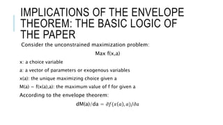
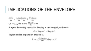
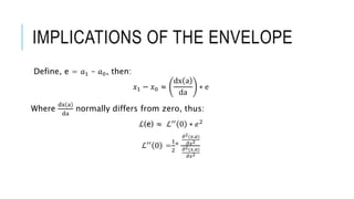
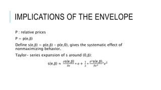
Akerlof and Yellen discuss the impact of small deviations from rational behavior on economic equilibria, highlighting how decision biases can affect market dynamics, such as the persistence of cartels and the business cycle. They explore the implications of the envelope theorem, near-rational behavior in exchange economies, and the consequences of monopolistic behavior and money supply shocks on welfare. The conclusion emphasizes the significant welfare and policy implications resulting from the identified decision biases.

1. CAN SMALL DEVIATIONS FROM
RATIONALITY MAKE
SIGNIFICANT DIFFERENCES TO
ECONOMIC EQUILIBRIA?
George A. Akerlof and
Janet L. Yellen

2. OUTLINE
Introduction
Implications of the Envelope Theorem
Near-Rational Behavior in a Pure Exchange Economy
The Welfare Effects of Near-Rational Behavior in the presence of
Distortions
 Monopoly and Technical Change
 The welfare Consequences of Money Supply Shocks
Conclusion

3. INTRODUCTION
Is a small amount of nonmaximizing behavior by agents capable if
causing changes in the equilibrium in the system?
As we saw in the lectures by Dr. Fatemi, There’re serious decisions
biases such as inertia, rules of thumb , …
These biases can be accounted for phenomena that have been
puzzling in the context of economic theory based strict maximization
such as the persistence of cartels and the existence of the business
cycle.
Fundenberg(1982), Kreps(1982), Rander(1980), Waldman(1985),
Russell and Thaler(1985) have examined the effects of other decision
biases on the equilibrium of an economy.

4. IMPLICATIONS OF THE ENVELOPE
THEOREM: THE BASIC LOGIC OF
THE PAPER
Consider the unconstrained maximization problem:
Max f(x,a)
x: a choice variable
a: a vector of parameters or exogenous variables
x(a): the unique maximizing choice given a
M(a) = f(x(a),a): the maximum value of f for given a
According to the envelope theorem:
dM(a)/da = 𝜕𝑓(𝑥 𝑎 , 𝑎)/𝜕𝑎

5. IMPLICATIONS OF THE ENVELOPE
𝑑𝑀(𝑎)
𝑑𝑎
=
𝜕𝑓(𝑥,𝑎)
𝜕𝑥
𝑑𝑥(𝑎)
𝑑𝑎
+
𝜕𝑓(𝑥 𝑎 ,𝑎)
𝜕𝑎
Of F.O.C, we have:
𝜕𝑓(𝑥,𝑎)
𝜕𝑥
= 0
A agent behaving inertially, leaving x unchanged, will incur
ℒ = f(𝑥1, 𝑎1) – f(𝑥0, 𝑎1)
Taylor-series expansion around 𝑥1:
ℒ ≈
1
2
(
𝜕2 𝑓(𝑥1,𝑎1)
𝜕𝑥2 )∗(𝑥0−𝑥1)2

6. IMPLICATIONS OF THE ENVELOPE
Define, e = 𝑎1 – 𝑎0, then:
𝑥1 − 𝑥0 ≈
dx a
da
∗ e
Where
dx a
da
normally differs from zero, thus:
ℒ(e) ≈ ℒ′′ 0 ∗ 𝑒2
ℒ′′
0 =
1
2
*
𝜕2(𝑥,𝑎)
𝜕𝑥2
𝜕2(𝑥,𝑎)
𝜕𝑥2

7. IMPLICATIONS OF THE ENVELOPE
P : relative prices
P = p(e,β)
Define s(e,β) = p(e,β) - p(e,0), gives the systematic effect of
nonmaximizing behavior.
Taylor- series expansion of s around (0,β):
s(e,β) ≈
𝜕s(e,β)
𝜕𝑒
∗ e +
1
2
∗
𝜕2s(e,β)
𝜕𝑒2 *𝑒2

8. NEAR-RATIONAL BEHAVIOR IN A PURE
EXCHANGE ECONOMY
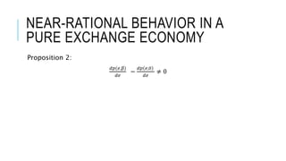
Proposition 1:
𝑑𝑈 𝑚
𝑑𝑒
=
𝑑𝑈 𝑛
𝑑𝑒
𝑑𝑉 𝑚
𝑑𝑒
=
𝑑𝑉 𝑛
𝑑𝑒
𝑈 𝑚(e,β) = u(p(e, β),𝑥1
−
+p(e, β) 𝑥2
−
(1 + 𝑒))
𝑑𝑈 𝑚
𝑑𝑒
= λ1[𝑝 𝑜 𝑥2
−
+(𝑥2
−
-𝑥2
𝑜
)
𝑑𝑝
𝑑𝑒
]

9. NEAR-RATIONAL BEHAVIOR IN A
PURE EXCHANGE ECONOMY
Proposition 2:
𝑑𝑝(𝑒,β)
𝑑𝑒
−
𝑑𝑝 𝑒,0
𝑑𝑒
≠ 0

10. Monopoly and Technical Change
𝑄1- 𝑄0 =
𝑐𝑒
2𝑏
The profit loss =
𝑐2 𝑒2
4𝑏
∶ 𝑡ℎ𝑒 𝑎𝑟𝑒𝑎 𝑜𝑓 𝐺𝐽𝐻
The difference between deadweight losses:
(𝑃 𝑜
−𝑐) ∗
𝑐𝑒
2𝑏
: BJHC

11. The welfare Consequences of Money
Supply Shocks
The Initial Equilibrium:
U = (M/P)
α
𝐺1−α
S.t. M + PG = 𝑀0
−
+ 𝑃𝐺−
𝑃 𝑜
= (1 − α) 𝑀0
−
/ α𝐺−
The sock: Money rain
For maximizers: 𝑀 𝑚 = α(𝑃𝐺−+ 𝑀0
−
(1+e))
Market clearing condition: β𝑀0
−
+(1- β) α(𝑃(𝑒, β)𝐺−
+ 𝑀0
−
(1+e))=
𝑀0
−
(1+e)

12. THE WELFARE CONSEQUENCES OF
MONEY SUPPLY SHOCKS
Define θ = (𝑃 𝑒, β − 𝑃 𝑜)/𝑃 𝑜
In the new EQU: θ =
1−𝛼(1−𝛽)
1−𝛽 −𝛼(1−𝛽)
*e > e, for 0 < β < 1
Now, we should compute the loss in the average utility. Equivalently,
this can be seen in the loss of utility of the average person.
For this person, G is not changed and M/P declines e(
𝑑𝜃
𝑑𝑒
− 1).Thus,
𝑑𝑈 𝑎𝑣𝑒𝑟𝑎𝑔𝑒 𝑝𝑒𝑟𝑠𝑜𝑛
𝑑𝑒
= −𝛼(
𝑑𝜃
𝑑𝑒
− 1) = -
𝛼𝛽
(1−𝛼)(1−𝛽)
𝛼: the elasticity of utility with respect to money,
𝑑𝜃
𝑑𝑒
− 1: percentage
change in money balances due to 1 percent change in the money
supply

13. CONCLUSION
There are serious welfare and policy implications due to decision
biases identified.