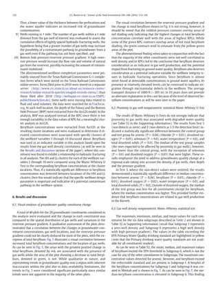
1) A geospatial model of the Barnett Shale region was created using GIS software to analyze groundwater quality data and determine if variations are associated with hydraulically fractured gas wells.
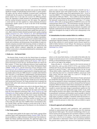
2) The study found that elevated concentrations of certain groundwater constituents, including beryllium, are likely related to natural gas production and beryllium could be used as an indicator of fracturing impacts.
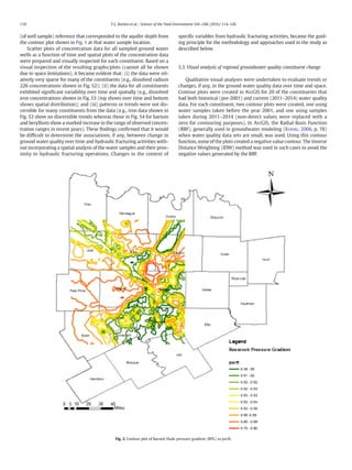
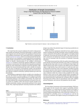
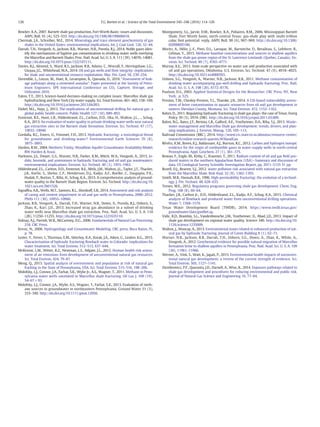
3) Results also indicated that gas well density and formation pressures correlate to changes in regional water quality, whereas proximity to gas wells alone does not, providing indirect evidence that micro annular fissures may transport fluids from fractured wells to groundwater.