1. The document discusses the formulation of a per capita population growth rate model that accounts for behaviors such as an initial increase then decline in growth rate and the Allee effect. 2. A per capita growth rate model is developed based on an existing logistic growth model, relating per capita growth rate to population size. 3. A local stability analysis of the critical points (N=0, N=C, N=K) shows that populations sizes of 0 and K are stable, while C is unstable, resulting in an S-shaped phase line graph.

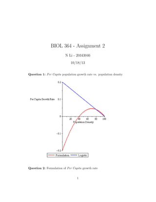
1. BIOL 364 - Assignment 2
N Li - 20343046
10/18/13
Question 1: Per Capita population growth rate vs. population density
Question 2: Formulation of Per Capita growth rate
1

2. Behaviours that need to be accounted for:
1. rate of decline is curvilinear
2. decline is not monotonic
3. Per Capita growth rates increase at low population levels, then
decline later
4. Allee effect accounted for
We consider an existing model for our formulation:
1
N
dN
dt
= r
N
C
− 1 1 −
N
K
(1) (1)
where:
• N: population level
• C: critical population size
• K: carrying capacity
• r: biological rate of growth
For completeness, we impose the biological constraint requiring: 0 < C < N
Putting the Per Capita growth rate in functional form, we have:
Rp-c = r
N
C
− 1 1 −
N
K
(2)
note: This formulation satisfies all required behaviours (see question 1)
Question 3: Inclusion of Per Capita growth rate into Logistic model
To begin, we’ll work off of the the logistic model. We see that the following
relation is true:
Rp-c
N
C
− 1
= r 1 −
N
K
(3)
2

3. To simplify expression (3), let’s define a new parameter δ = N
C
− 1
With this simplification, we can relate the formulation to the logistic model
by the following:
dNlogistic
dt
=
NRp-c
δ
(4)
Question 4: Phase-Line analysis
To begin, recall:
dN
dt
= rN
N
C
− 1 1 −
N
K
The critical pts are:
N*
= 0, C, K
From which, the following phase-line graph can be generated:
note: for details see question 5
Question 5: Local Stability analysis
Using the condition for local stability of continuous time models, we have:
df
dN
N = N*
< 0 (5)
where f is given by:
3

4. f = rN
N
C
− 1 1 −
N
K
(6)
Carry out the expansion:
f = r
N2
C
−
N3
CK
− N +
N2
K
(7)
Then:
df
dN
=
2rN
C
−
3rN2
CK
− r +
2rN
K
(8)
It follows that:
1. df
dN N =0
= −r < 0, =⇒ r > 0 is stable
2. df
dN N =C
= r − 1 < 0, =⇒ r < 1 is stable
3. df
dN N =K
= r(1 − K
C
) < 0, =⇒ r > 0 is stable
Analysis
1. d
dt
≈ df
dN N =0
gets smaller for r > 0
2. d
dt
≈ df
dN N =C
gets larger for r > 1
3. d
dt
≈ df
dN N =K
gets smaller for r > 0
These stability conditions =⇒
1. N*
= 0: Perturbations decrease, so 0 is stable
2. N*
= C: Perturbations increase, so C is unstable
3. N*
= K: Perturbations decrease, so K is stable
Together, these results give rise to the Phase-Line in question 4.
4

5. References
[1] Allee effect Model
http://en.wikipedia.org/wiki/Allee_effect(1) ∴
5