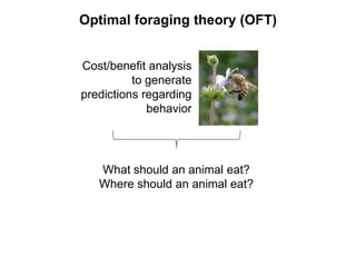
Cost/benefit analysis
to generate
predictionsregarding
behavior
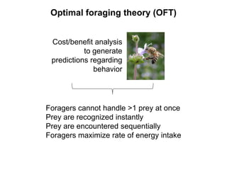
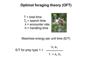
Optimal foraging theory (OFT)
Foragers cannot handle >1 prey at once
Prey are recognized instantly
Prey are encountered sequentially
Foragers maximize rate of energy intake
4.
Optimal foraging theory(OFT)
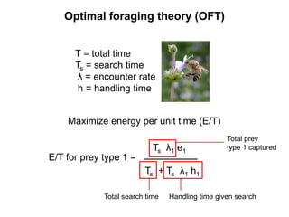
E/T for prey type 1 =
Ts λ1 e1
Ts + Ts λ1 h1
Maximize energy per unit time (E/T)
T = total time
Ts = search time
λ = encounter rate
h = handling time
Total prey
type 1 captured
Total search time Handling time given search
5.
Optimal foraging theory(OFT)
E/T for prey type 1 =
λ1 e1
1 + λ1 h1
Maximize energy per unit time (E/T)
T = total time
Ts = search time
λ = encounter rate
h = handling time
6.
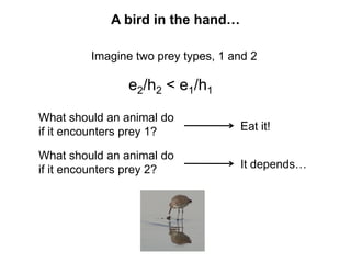
A bird inthe hand…
Imagine two prey types, 1 and 2
e2/h2 < e1/h1
What should an animal do
if it encounters prey 1? Eat it!
What should an animal do
if it encounters prey 2? It depends…
7.
A bird inthe hand…
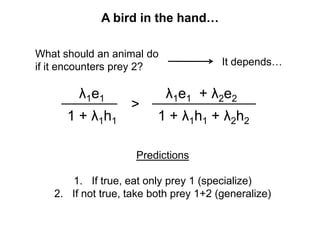
What should an animal do
if it encounters prey 2? It depends…
Predictions
1. If true, eat only prey 1 (specialize)
2. If not true, take both prey 1+2 (generalize)
λ1e1
1 + λ1h1
>
λ1e1 + λ2e2
1 + λ1h1 + λ2h2
8.
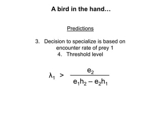
Predictions
3. Decision tospecialize is based on
encounter rate of prey 1
4. Threshold level
λ1 >
e2
e1h2 – e2h1
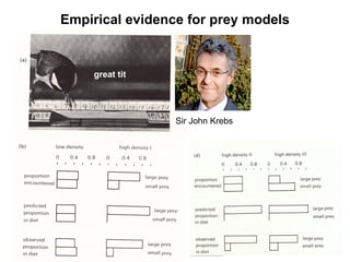
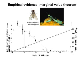
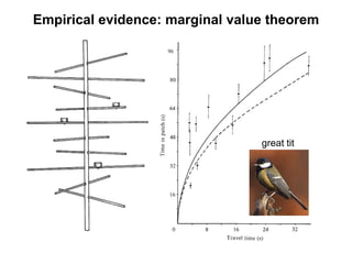
A bird in the hand…
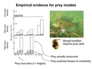
Empirical evidence forprey models
Bluegill predator
Daphnia prey (left)
Prey size class (I = largest)
Prey actually consumed
Prey predicted based on availability
Low
prey
density
High
prey
density
High
prey
density
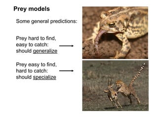
Prey easy tofind,
hard to catch:
should specialize
Prey hard to find,
easy to catch:
should generalize
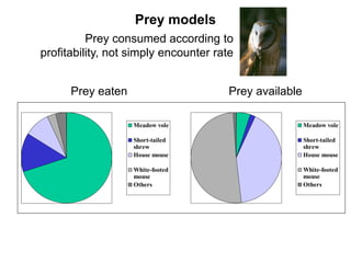
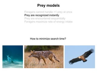
Prey models
Some general predictions:
13.
Foragers cannot handle>1 prey at once
Prey are recognized instantly
Prey are encountered sequentially
Foragers maximize rate of energy intake
Prey models
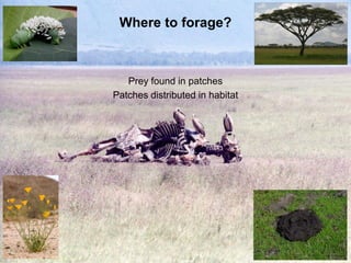
How to minimize search time?
14.
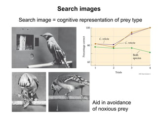
Search image =cognitive representation of prey type
Search images
Aid in avoidance
of noxious prey
15.
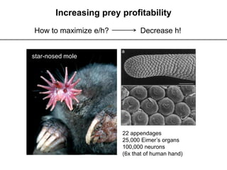
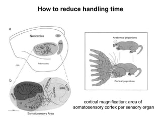
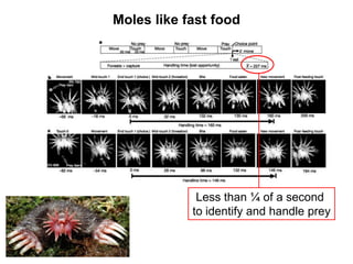
Increasing prey profitability
Howto maximize e/h? Decrease h!
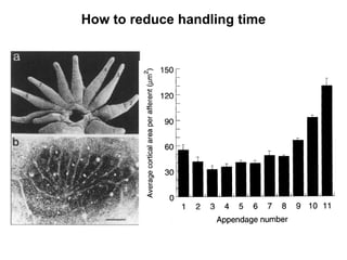
22 appendages
25,000 Eimer’s organs
100,000 neurons
(6x that of human hand)
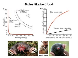
star-nosed mole
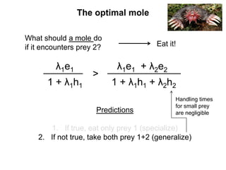
What should amole do
if it encounters prey 2? Eat it!
λ1e1
1 + λ1h1
>
λ1e1 + λ2e2
1 + λ1h1 + λ2h2
Predictions
1. If true, eat only prey 1 (specialize)
2. If not true, take both prey 1+2 (generalize)
Handling times
for small prey
are negligible
The optimal mole