2. 238 J.H. Tarnecki et al. / Fisheries Research 179 (2016) 237–250
This paper works to overcome multiple statistical issues of
preparing diet matrices for an Atlantis ecosystem model, or any
other subsequent analyses, using data from the Gulf of Mexico as
a case study. We first combine data from literature and empirical
studies to facilitate identifying sparse predator–prey linkages that
were missing from previous work (Masi et al., 2014). Second, we
recategorize predators and prey into functional groups more suit-
able for end-to-end ecosystem models using principle coordinate
analysis. Third, we overcome the lack of uncertainty estimates by
bootstrapping the aggregate diets of fish then statistically quan-
tifying the diet estimates and associated error (Ainsworth et al.,
2010). We compare the estimated diet matrix to diet matrices pre-
viously described for the region. Finally, we assess the performance
of an end-to-end Atlantis ecosystem model for the Gulf of Mexico
utilizing the revised diet matrix.
2. Methods and materials
2.1. Functional groups and data sources
We analyze diet information of 48 predator functional groups
(Table 1). The analysis of Masi et al. (2014) was augmented by (1)
recategorizing predator and prey species into functional groups
based on ecological factors, and (2) incorporating data (Table 2)
from a larger spatial area to represent the feeding ecology relevant
to the whole GOM. Diet data were obtained from: (1) Florida Fish
and Wildlife Conservation Commission’s (FWC’s) Fisheries Inde-
pendent Monitoring (FIM) group based in St. Petersburg, Florida;
(2) GoMexSI database (Simons et al., 2013) developed by Texas
A&M University in Corpus Christi, Texas (http://gomexsi.tamucc.
edu/); (3) diet information acquired through Fishbase.org (Froese
and Pauly, 2013); (4) dissections performed by Masi et al. (2014),
and (5) diet studies of longline-caught fish collected by the Univer-
sity of South Florida (USF; S. Murawski, Pers. Comm.).
The statistical analysis considers only fish. However, we did
obtain diet information pertaining to marine mammals, turtles,
Table 1
Functional groups and number (no.) of viable stomachs containing identifiable prey
and used in diet analysis. Functional groups containing asterisk (*) are composed of
a single species.
Functional groups, (no. of stomachs) Functional groups (continued)
Benthic Feeding Sharks, (n = 21) Other Demersal Fish (n = 2113)
Bioeroding Fish, (n = 30) Other Tuna (n = 6)
*Black Drum (n = 26) *Pinfish (n = 133)
*Blacktip Shark (n = 32) *Pompano (n = 22)
*Blue Marlin (n = 2) *Red Drum (n = 1440)
*Bluefin Tuna (n = 22) *Red Grouper (n = 440)
Deep Serranidae (n = 63) *Red Snapper (n = 134)
Deep Water Fish (n = 11) *Scamp (n = 15)
Filter Feeding Sharks (n = 1) Sciaenidae (n = 300)
Flatfish (n = 846) Seatrout (n = 1270)
*Gag Grouper (n = 1216) Shallow Serranidae (n = 922)
*Greater Amberjack (n = 24) *Sheepshead (n = 11)
Jacks (n = 299) Skates and Rays (n = 125)
*King Mackerel (n = 125) Small Demersal Fish (n = 2155)
*Ladyfish (n = 69) Small Pelagic Fish (n = 163)
Large Pelagic Fish (n = 66) Small Reef Fish (n = 573)
Large Reef Fish (n = 440) Small Sharks (n = 23)
Large Sharks (n = 116) *Snook (n = 1317)
*Little Tunny (n = 1) *Spanish Mackerel (n = 143)
Lutjanidae (n = 2166) *Spanish Sardine (n = 55)
Medium Pelagic Fish (n = 21) *Swordfish (n = 9)
Menhaden (n = 17) *Vermillion Snapper (n = 671)
Mullets (n = 61) *White Marlin (n = 2)
Other Billfish (n = 1) *Yellowfin Tuna (n = 1)
birds, and invertebrate species from online sources includ-
ing: Animaldiversity.org (Myers et al., 2015) and Sealifebase.org
(Palomares and Pauly, 2015), to form a complete picture of the
GOM food web. Collectively, this study’s compiled dataset repre-
sents the feeding ecology of predators throughout the GOM and
will be referred to as the ‘revised’ food web matrix hereafter. In
total, 17,719 fish belonging to 474 unique species were analyzed for
this study. Capture locations were provided for FWC and GoMexSI
Fig 1. Catch locations of the Gulf of Mexico Species Interactions (GoMexSI) and Florida Fish and Wildlife Conservation Commission (FWC) samples in the Gulf of Mexico.
3. J.H. Tarnecki et al. / Fisheries Research 179 (2016) 237–250 239
Table 2
Capture location(s), unit of measure, number (no.) of samples, and number of species for each data.
Data source Location of catch Weight (g), vol., % Diet No. of samples No. of species
FWC Primarily west coast of Florida, restricted to the Florida shelf Vol. 16,220 166
GoMexSI Primarily western and northern Gulf of Mexico Vol. 592 117
Fishbase No locations specified % Diet 867 330
Masi et al., 2014 Gulf wide sampling efforts Weight (g) 25 7
USF Gulf wide sampling efforts Weight (g) 15 7
Total 17,719 474 Unique spp.
Source: Florida Fish and Wildlife Conservation Commission (FWC), Gulf of Mexico Species Interaction Database (GoMexSI), Fishbase.org studies (), Masi et al. (2014), and the
University of South Florida (USF). Raw data was measured in either weight (g), Volume (Vol.) or percent diet (% Diet).
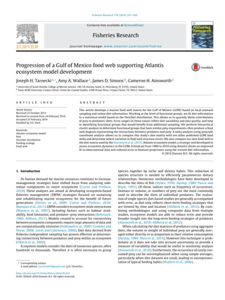
Fig. 2. Hierarchical cluster analysis showing diet similarity by functional group.
Dashed lines indicate statistically similar predators and black brackets illustrate
similar clusters of predators. Black brackets at 0% dissimilarity indicate identical
predator–prey relationships (e.g. white, brown, and pink shrimp functional groups).
Number of hierarchical clusters is 25.
samples (Fig. 1), but were not specified for Fishbase, USF studies,
or non-fish groups (only indicated as GOM).
2.2. Statistical model
A statistical analysis was applied to the composition data which
bootstraps the diet of each functional group and fits the normalized
data to a Dirichlet distribution (Ainsworth et al., 2010). As a first
step, we arranged the normalized predator diets into an 89 × 89
matrix, using predator versus prey Atlantis functional groups to
describe interaction. The most-frequently observed diet values
were most often zero as it is unlikely for a predator to feed across
a large proportion of the 89 prey categories. To correct for zero
inflated data we adopted the methodology of Masi et al. (2014).
We randomly selected 15% of the total number of stomachs for
a given functional group and averaged the diet values together.
This creates a pseudo predator stomach that should represent a
time-integrated diet composition. We then bootstrapped 10,000
such samples with replacement and fit the bootstrapped values to
the Dirichlet density function using a maximum likelihood fitting
procedure (Ainsworth et al., 2010; Masi et al., 2014). The Dirich-
let function is the multivariate generalization of the beta function.
Thus, the marginal beta distributions provide us with a mode, rep-
resenting the most frequently observed diet proportion for that
predator–prey combination in percentage wet weight, as well as
confidence intervals.
There are 89 potential prey functional groups (corresponding to
functional groups of the GOM Atlantis model). If we let p denote
a random vector of i = 89 prey item proportions that sum to one,
I
pi = 1, and whose elements are greater than or equal to zero,
pi ≥ 0, then we can express the probability density at pi with a
parameter vector ˛ using the Dirichlet function (Eq. (1)):
p(a)∼f (p1, p2, . . ., pI)|˛1, ˛2, . . ., ˛I) =
( IaI)
I (˛I) i
p˛i−1
(1)
vector ˛ is estimated from a set of training data (bootstrapped data
to which the statistical model is fit) representing diet proportions
D = {p1, . . ., pN} using a maximum likelihood fitting procedure that
maximizes p (D|˛) = I
p (pi|␣I). We employed VGLM in the VGAM
package (Yee and Wild, 1996) in the R statistical environment (R
Core Team, 2015).
2.3. Hierarchical clusters analysis
A dendrogram of predator diets was created using hierarchical
clustering analysis (Clarke et al., 2008; Masi et al., 2014) and Bray-
Curtis measures of distance (Bray and Curtis, 1957) between diets.
First, the Bray-Curtis dissimilarity measure was computed between
each pair of samples (j and k):
Djk =
n
i=1
|yij − yik|
n
i=1
yij + yik
(2)
4. 240 J.H. Tarnecki et al. / Fisheries Research 179 (2016) 237–250
Table3
Congruencymatrixcomparingthepredator–preyrelationshipsoftherevisedfoodwebmatrixandotherknownGulfofMexicofoodwebsmatrices’.Percentcongruencywasanalyzedwithbinaryconnectivitymetricsfollowing
similarityprofileroutine(SIMPROF)testperClarkeetal.(2008)atasignificancelevelofP≤0.05.
Revised
matrix
Careyetal.,
2013
Chagaris
(2013)
Dynamic
Solutions
2013
Geersetal.,
2014
Grüssetal.,
2014
Luczkovich
etal.,2002
Minello
(unpublished
data)
Okeyand
Mahmoudi
2002
Passarella
andHopkins
1991
Waltersetal.,
2006
Revisedmatrix
Careyetal.,201317.4
Chagaris(2013)20.433.1
DynamicSolutions201340.584.571
Geersetal.,20142.613.450.246.5
Grüssetal.,201477.943.320.41.81.7
Luczkovichetal.,200234.385.791.27068.24.8
Minello(unpublisheddata)40.889.462.68119.112.396.4
OkeyandMahmoudi200233.216.458.55810.34.782.141
PassarellaandHopkins199171.485.769.25036.433.333.371.475
Waltersetal.,200643.745.38070.838.913.472.257.645.375
where yij is the count of the ith species in the jth sample, yik is
the count of the ith species in the kth sample, and n is the num-
ber of species. Cluster analysis was performed on the dissimilarity
measures by computing the cluster mode group averages along
with similarity profile analysis (SIMPROF; Clarke et al., 2008) with
999 permutations to produce significant (P < 0.05) aggregations of
predator groups as hierarchical clusters.
2.4. Comparison of the revised food web to other models
This study’s revised diet matrix was compared to the diet matri-
ces used by ten other Gulf-wide multispecies models (Passarella
and Hopkins, 1991; Luczkovich et al., 2002; Okey and Mahmoudi,
2002; Walters et al., 2006; Carey et al., 2013; Chagaris, 2013;
Dynamic Solutions, 2013; Geers et al., 2014; Grüss et al., 2014; T.
Minello, National Oceanic and Atmospheric Administration (NOAA)
Pers. Comm.). For the comparisons, larval stages were omitted and
only juvenile and adult predator diets were considered. To facilitate
comparisons, functional groups and species within each study were
aggregated into 13 ‘supergroups’: Benthic Fauna, Cephalopods,
Deepwater Fish, Elasmobranchs, Inshore Fish, Marine Mammals,
Pelagic Fish, Mollusks and Echinoderms, Planktonic Fauna, Reef
Associated Fish, Seabirds, Reef Dependent Fish, and Turtles. Super-
groups were chosen based on no particular basis, but rather to
simply aggregate the diverse datasets into one broad matrix for
comparisons. Additionally, the diet compositions for each super-
group were normalized.
To facilitate comparisons between studies, we performed a one-
way Analysis of Similarities (ANOSIM) with 999 permutations to
compare the aggregated normalized diets for each supergroup
between studies. These results were compiled using a respective
binary connectivity matrix to reveal congruence. The ‘congruency
matrix’ enumerates percent similarity of one study to another.
Within the congruency matrix, 100% congruence implies all
predator–prey relationships are identical between studies whereas
0% implies complete dissimilarity among predator–prey feeding
ecology. A 2D Multidimensional Scaling (MDS) scatterplot cre-
ated from the percent similarity illustrates the findings. Tightly
clustered points indicate similar food webs and broad clustering
indicates dissimilar food webs.
To compare individual supergroup diets from this study with the
ten other studies, predator similarity was tested in the Primer sta-
tistical package (ver. 6) using Principal Coordinates (PCO) graphs
(Anderson and Willis, 2003). The Bray-Curtis similarity measure
was calculated between each pair of samples then plotted to
describe variation on two axes.
2.5. Comparison of the revised matrix with Atlantis
Atlantis is a biogeochemical marine ecosystem model repre-
senting ocean physics, nutrient cycling, high trophic level dynamics
and fisheries, in three spatial dimensions. Fulton et al. (2007) pro-
vide a thorough fisheries management application in Australia, and
Fulton et al. (2011) present a meta-analysis of global applications.
The best resources for the theory and code are Fulton (2001, 2004)
and Link et al. (2011).
Rather than using diet proportions, Atlantis’ trophic model is
based on ‘availability’ parameters, a scaling value in a Type II
predator–prey functional response (see Eq. 69 in Link et al., 2011).
Availability reflects total consumption potential in addition to diet
preference. Therefore, it is sensitive to functional group aggre-
gation, predator and prey abundance, spatial co-occurrence and
other factors, and the availabilities matrix must be tuned as part of
the calibration process. There are conventions on how initial esti-
mates can be derived from diet proportion data. Gamble (Northeast
5. J.H. Tarnecki et al. / Fisheries Research 179 (2016) 237–250 241
Fig. 3. Food web diagram illustrating predator–prey connectivity in the Gulf of Mexico. Each box represents a cluster from the hierarchical cluster analysis and is named after
the predator functional group containing the highest biomass estimates, provided by Drexler and Ainsworth (2013). Boxes are proportional to area log biomass estimates
and arrows indicate the flow of energy from prey to predator. Dotted lines indicate groups with ≥10% − 20% prey contributions, thin solid lines represent prey contributions
ranging from >20% − 40%, and thick solid lines indicate >40% prey contributions. Diets <10% were omitted from the diagrams. Estimated trophic level of each grouping is
indicated on the Y-axis.
Fig. 4. 2D Multidimensional Scaling (2D-MDS) plot of area cluster congruency matrix. Symbols (representing GOM models) use spatial distribution to represent similarities
in predator–prey relationships. The degree of correspondence between the distances among point values or ‘stress’ is 0.14.
Fisheries Science Center-NOAA, Pers. Comm.) developed method-
ology to estimate availabilities numerically (for applications, see:
Ainsworth et al., 2011; Link et al., 2011). Brand et al. (2007) and
Ainsworth et al. (2015) started with low, medium and high sets of
values to approximate total flows. Later revisions of the Brand et al.
(2007) model scaled proportional diet data to a desired mean (I.
Kaplan, Northwest Fisheries Science Center-NOAA, Pers. Comm.).
The connectivity pattern is generally informed by diet data.
Ainsworth et al. (2015) developed an Atlantis model of the
GOM using a food web provided by Masi et al. (2014) as the basis
of representing the availabilities matrix. In this study, we com-
pare our updated and revised diet matrix against the (calibrated)
Ainsworth et al. (2015) diet matrix rather than the uncalibrated
Masi et al. (2014) matrix, and conduct Atlantis simulations (below)
that maintain the absolute flows of the Ainsworth et al. (2015)
model changing only the pattern of connectivity to represent the
new data. There is a theoretical justification for this. If we were to
replicate the entire tuning procedure, improvements in model fit
would reflect not only the improved diet information but also the
(rather subjective) tuning process. Thus, the value of the new data
would not be clearly discernable. In contrast, a comparison can be
made if we maintain in Atlantis the absolute magnitude of flows
that were tuned by Ainsworth et al. (2015) and have been shown
to yield realistic model behavior.
6. 242 J.H. Tarnecki et al. / Fisheries Research 179 (2016) 237–250
Fig. 5. Principle coordinates (PCO) panel plots illustrating similarities between the revised food web matrix (black symbols) and other multispecies models’ (gray symbols)
predator–prey relationships.
To address the comparisons between the Ainsworth et al.
(2015) availabilities matrix with the current diet information, we
compared presence/absence of prey and percent contribution to
determine differences in connectivity. To streamline this analysis,
prey items were broadly classified into four supergroups: Elasmo-
branchs, Large Pelagic Fishes, Reef Fishes and Nearshore/Inshore
Fishes. Comparisons in volume and prey composition were made
both visually and by using similarity percentages (SIMPER), which
provides a measure of resemblance between studies (Clarke et al.,
2008). High percentages indicate prey contribution and volume
are similar between studies, while low percentages indicate high
variability between studies.
Canonical analysis of principal coordinates (CAP) was performed
using Primer to illustrate supergroup similarity in the Atlantis
model and to illustrate how the incorporation of this study’s revised
diet data could improve supergroup correlation (see Anderson
and Willis (2003) for a full description of CAP methodology). We
applied the Bray-Curtis dissimilarity measure to the diet matri-
ces for Atlantis and Atlantis + revised food web. CAP was then used
to constrain the ordination of data points. Within each CAP plot,
clustering indicates similarity in diet composition. These similar-
ities in feeding ecology are represented within supergroups and
among predator functional groups. Groups clustered together indi-
cate greater similarity in feeding behavior than compared to groups
that do not cluster.
Finally, we ran a hindcast (following Ainsworth et al., 2015)
from 1980 to 2010 and compared functional group biomass pro-
jections against observed biomass time series data (see Ainsworth
et al. (2015) for data sources). The fit against this scaled observed
biomass data is measured by the sum of squared residuals (SS)
where [SS =
n
i=1
ˆYi − Yi
2
] and where ˆYi is predicted biomass
in year i, Yi is observed biomass and n is total simulation years
(n = 30). We also employed discrepancy as a metric of model skill
7. J.H. Tarnecki et al. / Fisheries Research 179 (2016) 237–250 243
[discrepancy =
2010
i=1990
ˆYi − Yi ]. Low values of SS and discrep-
ancy near zero indicate good model performance. We consider the
years 1990 to 2010 when calculating these metrics to discount early
transient dynamics.
We ran three simulations using the GOM Atlantis model: (1)
recreating the simulations of Ainsworth et al. (2015) using their
original diet matrix, (2) employing a revised diet matrix that
included trophic linkages identified in this study but absent in
Ainsworth et al. (2015), and (3) employing a revised diet matrix
that included this study’s new trophic linkages but also eliminated
linkages used by Ainsworth et al. (2015) that were not confirmed
by the current study. These scenarios are referred to as ‘Original,
“Revised A” and ‘Revised B’ hereafter. Where new trophic linkages
were required, we assumed a strength of interaction similar to the
mean interaction strength experienced by a given prey across all
its predators.
3. Results
3.1. Diet matrix
Diet proportions of predators in the GOM are highly variable
and range from including a single functional group to 15 different
functional groups (see Supplementary Appendix I for diet esti-
mates and 95% confidence intervals). The greatest diversity in prey
was observed for the functional group Pinfish (Lagodon rhomboids,
Sparidae), which included various fishes, shrimps, bivalves, plank-
ton, and detritus. Filter Feeding Sharks exhibited the least diverse
feeding strategy and fed exclusively on phytoplankton.
3.2. Hierarchical clusters and food web diagram
Hierarchical cluster analysis conducted on revised matrix
yielded (n = 25) unique hierarchical clusters (Fig. 2), ranging
Fig. 6. Diet comparisons between the Ainsworth et al. (2015) Atlantis model diet data and the revised diet data. Predator functional groups are listed vertically and prey
functional groups are listed horizontally. Gray boxes refer to prey linkages that were present in Ainsworth et al. (2015), while black boxes indicate new prey linkages.
Predators are presented in order of number of missing linkages.
8. 244 J.H. Tarnecki et al. / Fisheries Research 179 (2016) 237–250
Fig. 6. (Continued)
from one to ten predator functional groups per cluster. Clusters
containing one functional group displayed statistically differ-
ent (P < 0.05) feeding behaviors relative to all other functional
groups. These include: Spanish Sardines (Sardinella aurita, Clu-
peidae), Filter Feeding Sharks, Sponges, Small Pelagic Fish, Large
Pelagic Fish, and Bioeroding Fish. The largest aggregation of func-
tional groups (n = 10) present within a single cluster was observed
among the omnivorous fishes: Benthic Feeding Sharks, Deep Ser-
ranidae, Vermilion Snapper (Rhomboplites aurorubens, Lutjanidae),
Large Reef Fish, Flatfish, Sciaenidae, Red Drum (Sciaenops ocella-
tus, Sciaenidae), Shallow Serranidae, Lutjanidae, and Red Grouper
(Epinephelus morio, Serranidae). Feeding behavior displaying 0%
dissimilarity was observed between (1) Crabs & Lobsters and Stone
Crabs, (2) White Shrimp (Litopenaeus setiferus, Penaeidae), Brown
Shrimp (Farfantepenaeus aztecus, Penaeidae), and Pink Shrimp
(Penaeus duorarum, Penaeidae), and (3) Oysters and Sessile Filter
Feeders, indicating very similar diets with no discernable differ-
ences within the context of this analysis. The cluster exhibiting
the greatest dissimilarity between functional groups was observed
among the large pelagic fishes. Within this cluster, the diet of Other
Billfish was 86% dissimilar to the other functional groups. This was
in part due to low sample size (n = 1) and high consumption (46%)
of Spanish Mackerel (Scomberomorus maculatus, Scombridae). All
other groups within large pelagic fish cluster foraged primarily
(46–73%) on Deepwater Fish.
Each hierarchical cluster represents a box used in the GOM
food web diagram (Fig. 3). Base-level prey (Phytoplankton,
Plants/Macroalgae, Octocorals, and Detritus) that were not present
in hierarchical clusters were added to the food web diagram
to complete essential linkages. These base-level prey functional
groups represented the lowest trophic levels while Other Tuna
and King Mackerel represented the highest aggregated trophic lev-
els. Species included within ‘Other Tuna’ (Blackfin Tuna, Thunnus
atlanticus; and Bluefin Tuna, Thunnus thynnus) were primarily feed-
ing on Large Pelagic Fish, Small Pelagic Fish, and Squid. Species
included within ‘King Mackerel’ (King Mackerel, Scromberomorus
cavalla, Scombridae; Little Tunny, Euthynnus alletteratus, Scombri-
dae; and Spanish Mackerel) fed primarily on Small Pelagic Fish.
9. J.H. Tarnecki et al. / Fisheries Research 179 (2016) 237–250 245
3.3. Comparison of the revised matrix to other models
Congruency ranged from 1.7% to 96.4% among the models
(Table 3). The lowest congruency was between the Geers et al.
(2014) and Grüss et al. (2014) models, which compared the diets
of Inshore Fish, Pelagic Fish, and Reef Associated Fish. The compar-
ison between Luczkovich et al. (2002) with Minello (Pers. Comm.)
displayed the highest congruency (96.4%), but only evaluated the
diets of Inshore Fish.
Percent congruency comparing the revised matrix to the other
GOM models ranged from 2.6% to 77.9%, with Geers et al. (2014)
displaying the lowest congruency and Grüss et al. (2014) display-
ing the highest. These models contained a number of comparable
supergroups. However, Geers et al. (2014) contained more inshore
data. Overall, the revised matrix used the largest sample sizes and
greatest diversity of predators compared to the other GOM food
webs. Similarities between food webs are further illustrated using
a 2D MDS (Fig. 4). The diet matrices of Grüss et al. (2014) and
Passarella and Hopkins (1991) were most similar to the revised
matrix while Geers et al. (2014) was least similar.
The best fit PCO plot (Fig. 5) comparing supergroups between
studies had 50.8% variation on the X-axis, which is likely most influ-
enced by trophic level, and 32.4% variation on the Y-axis which is
likely most-influenced by feeding mode, as benthic feeding behav-
iors tend to be positioned low and pelagic feeding is positioned
high. Overall, the analysis displayed relatively tight cluster arrange-
ments for most supergroups. Pelagic Fish, Inshore Fish, and Reef
Fish all exhibited distinct cluster arrangements, while Elasmo-
branchs and Cephalopods exhibited broader clusters.
3.4. Comparison of the revised matrix with Atlantis
Diet comparisons were made to evaluate the presence versus
absence of prey across each predator functional group for the
Atlantis and revised datasets (Fig. 6). Considering only the diets
of fish predator functional groups, a total of 399 prey linkages
were identified as ‘missing’ when comparing Atlantis to the revised
dataset. Comparisons of the revised matrix with the Atlantis dataset
revealed 31% of all functional groups contained >10 missing link-
ages, 27% contained 6–10 missing linkages, and 42% contained ≤5
missing prey linkages. Of these, King Mackerel and the Spanish Sar-
dine (sample sizes n = 27 and n = 23) functional groups exhibited
the greatest number of missing prey, while Swordfish (sample size
n = 9) exhibited zero dissimilarity between datasets.
Stacked bar graphs and similarity percentages were used to
compare differences in fish diet composition between the revised
and Atlantis datasets (Fig. 7). Similarity ranged from 5.5% to 75.5%.
Of these, Menhaden (Brevoortia spp., Clupeidae) was the least
variable functional group overall. Menhaden diet was composed
primarily of pelagic fauna and detritus. However, Menhaden diet
Fig. 7. Percent diet and similarity percentages (SIMPER) of predator categories comparing the Ainsworth et al. (2015) Atlantis model diet data and the revised diet data.
Graphs were constructed for fish predator groups using prey grouped into 12 supergroups.
10. 246 J.H. Tarnecki et al. / Fisheries Research 179 (2016) 237–250
Fig. 7. (continued)
varied in percent composition between datasets. Benthic feed-
ing sharks displayed the lowest similarity between datasets. The
Atlantis dataset shows this group primarily consumed Elasmo-
branchs and Pelagic fauna, while the revised dataset indicates
Benthic Feeding Sharks consume mostly benthic prey (e.g. Crabs
and Lobsters, Shrimps, and Small Benthic Fauna). Overall, stacked
bar graphs show similar prey supergroups were consumed for most
comparable fish predators between datasets. Stacked bar graphs
coupled with similarity percentages provide insight on which func-
tional groups differ the greatest and therefore which functional
groups would presumably benefit from targeted sampling efforts.
CAP plots (Fig. 8) illustrate the potential improvements of
ecosystem connectivity to the Atlantis ecosystem model with the
integration of this study’s updated and revised dataset. Within each
graph, data points represent individual functional groups while
symbols represent the designation of a functional group into a par-
ticular supergroup. CAP plots display a measure of similarity on
both the X and Y-axis. This similarity ranged between −0.2 and
+0.3 on the X-axis, and −0.2 and +0.2 on the Y-axis for the Atlantis
model data. Similarity for the Atlantis + revised food web ranged
from −0.4 and +0.4 on both X and Y axes. For Atlantis (Fig. 8A) broad
clustering was observed among all supergroup fish categories indi-
cating prey resources were highly variable between individual
functional groups occupying the same supergroup. After integrat-
ing the revised data (Fig. 8B) tighter clustering was observed among
functional groups and greater distinction between supergroups.
The inclusion of the new diet information resulted in a modest
improvement in the Atlantis model performance. Under scenario
Revised A, 69% of the functional groups benefited from reduced
residuals relative to scenario Original. Under scenario Revised B,
59% of groups benefited. The median reduction in the SS was
14% for Revised A and 23% for Revised B indicating that we more
accurately captured interannual variability in population size. A
one-tailed Wilcoxin signed rank test for paired data indicates sig-
nificant improvement over the original model fit for both scenario
Revised A (p = 0.008) and scenario Revised B (p = 0.03). Under both
scenarios we observed a reduction in overall discrepancy; results
from revised B are shown in (Fig. 9). A 14% reduction in discrepancy
in Revised A and a 28% reduction in Revised B, relative to scenario
Original, suggests fewer systematic errors exist in model predic-
tions.
11. J.H. Tarnecki et al. / Fisheries Research 179 (2016) 237–250 247
Fig. 8. Canonical analysis of principal coordinates (CAP) plots illustrating (A) the distribution of the Ainsworth et al. (2015) Atlantis predator functional groups and (B) the
distribution of Atlantis + revised predator groups with respect to diet. Each symbol represents an Atlantis model functional group. Functional groups were categorized into
supergroups to identify similarities in feeding ecology.
4. Discussion
We combined the diets of predators from multiple sources and
formulated a new food web, improving on the earlier attempts by
Masi et al. (2014) and Ainsworth et al. (2015). Using the maxi-
mum likelihood fits of the Dirichlet distribution, we were able to
address issues noted by other authors concerning the overestima-
tion of rarely consumed prey (Walters et al., 2006; Ainsworth et al.,
2010). Within our revised dataset, sample sizes were small for most
functional groups. The statistical method employed here resulted in
wide confidence intervals in such cases, accurately characterizing
the uncertainty. Moreover, the diet proportion values used in the
final diet matrix represent the modes of the marginal beta distribu-
tions rather than the means, which down-weights the importance
of rarely consumed prey. This is advantageous when dealing with
small diet data sets of opportunistic predators.
The error range generated by this technique may be useful
for sensitivity analysis of diet parameters used in the ecosystem
modeling context. In some cases, the realized diet, which may be
affected by spatial and temporal overlap of predator and prey, han-
dling time, satiation and other non-linear effects, may be extracted
from the model during simulations (e.g., in Atlantis: Fulton et al.,
2007). A goodness of fit measure for the trophic model may be
derived by comparing the realized diet proportions to the maxi-
mum likelihood marginal beta distributions.
Hierarchical cluster analysis identified feeding guilds within
our dataset. While only the diets were considered for cluster
analysis, we observed a potential interaction between diet and
sampling location. Clusters were observed for predators occu-
pying similar habitats including: blue-water pelagic fishes (e.g.
tunas, billfishes), coastal pelagics (Pompano, Trachinotus carolinus,
Carangidae; Ladyfish, Elops saurus, Elopidae), reef associated fish
(snappers, groupers), as well as several other inshore and offshore
assemblages. These clusters were formed because of the consump-
tion of location-specific prey (e.g. tunas and billfishes consuming
deepwater fish). However, we also observed similar species that
occupy different clusters despite sharing commonalities in habitat
and feeding ecology. For example, Seatrout and Red Drum share
similarities in habitat preference. As juveniles and adults, both
species can be found in nursery habitat (e.g. mangroves, marshes,
etc.), and opportunistically feed on similar prey (Llanso et al., 1998).
In this study, cluster analysis grouped Red Drum with reef associ-
ated fishes (groupers, snappers and sea basses), and Seatrout with
bay and coastal predatory fish (Ladyfish, Pinfish, jacks).
Disparities such as these are likely attributed to habitat differ-
ences. Dennis and Bright (1988) report species assemblages differ
dramatically throughout the GOM, and therefore differences in
feeding ecology likely differ as well. In the northern panhandle of
Florida to the east coast of Texas, Red Drum occupy primarily sea-
grass habitat (Matlock, 1987). Within this study, fish were largely
collected in areas dominated by mangrove habitat and nearshore
natural hard bottom reefs. The northern and western GOM are con-
tain greater abundances of marsh and seagrass habitat (Stunz and
Minello, 2001; Rooker et al., 1998), as well as deeper natural hard
12. 248 J.H. Tarnecki et al. / Fisheries Research 179 (2016) 237–250
Fig. 9. Sum of squared residuals (SS) comparing the scenario Original (Ainsworth
et al., 2015) diet matrix to Revised B (this study’s revised matrix). Black bars indicate
model performance using original diet matrix and gray bars show the revised diet
matrix. Asterisk indicates improved fit. Median change: 23% reduction in SS.
bottom reefs and artificial habitats (Cowan et al., 2011). It is likely
that future sampling efforts focused in these areas would be needed
to uncover regional differences in predator–prey relationships.
Collectively, the revised diet matrix was most similar to other
‘offshore’ datasets such as those of Grüss et al. (2014) and Passarella
and Hopkins (1991). Specifically, these study’s compared the diets
of Inshore/Nearshore Fishes, Pelagic Fishes, and Reef Associated
Fishes. Dissimilarity was greatest within the Elasmobranchs super-
group in which diet composition varied depending on sampling
location and habitat. Within the Elasmobranchs supergroup we
reported the diets for nearshore skates and rays, along with a
diversity of shallow, pelagic, and deepwater sharks. Some models
sampled only coastal communities, therefore only shallow water
sharks and rays were reported, if at all. Among all models congru-
encies were highest among offshore food webs (96.4%; Luczkovich
et al., 2002 with Minello, Pers. Comm.), and differed the most when
comparing nearshore to offshore food webs (1.7%; Geers et al., 2014
with Grüss et al., 2014). This study’s revised food web contained
greater biodiversity in species composition relative to other food
webs and congruency consequently was lower when comparing
studies with few representatives within a supergroup.
Expanding the stomach data used in our diet matrix revealed
a large number of linkages missing from the Atlantis GOM food
web. Within our comparisons between Atlantis and the revised
food web matrix, we ranked these predators in order of number
of missing linkages such that predators exhibiting higher numbers
of missing linkages would be ideal candidates for future sam-
pling. Furthermore, we computed similarity between models to
provide additional insight to where additional sampling is needed.
For most predator functional groups the dominant prey items are
largely consistent between studies, but for others (especially Ben-
thic Feeding Sharks, Bioeroding Fish and Spanish Mackerel) the
dominant prey items varied. Several authors (Ferry and Cailliet,
1996; McCawley and Cowan, 2007; Llopiz and Cowen, 2009) indi-
cate large sample sizes taken over many years and seasons are
needed to account for variability in diet. Differences here are
likely attributed to low sample sizes or spatial differences between
datasets. Increases in sampling effort would be required to identify
the dominant prey as well as identify any seasonal, ontogenetic, or
habitat shifts that may influence prey consumption during the life
history of a predator (Cortés, 1997).
Integrating the new diet matrix into the Ainsworth et al. (2015)
Atlantis model led to supergroups becoming more distinct in what
they ate. Using the new diet information, both reconstruction
simulations, Revised A and Revised B, saw reduced residuals rela-
tive to time series observational biomass and reduced discrepancy
for a majority of functional groups. It should be noted that this
represents only a rough first application of this new diet data. Sub-
sequent model tuning has the potential to capitalize on this new
diet information further. Behavior of an Atlantis model depends
on several influential parameter sets besides the diet matrix (e.g.,
recruitment, consumption, growth rates). In the process of model
calibration, adjustment of all parameters is done simultaneously.
When Ainsworth et al. (2015) calibrated the model they did so
with the original (less accurate) diet matrix in place. Errors else-
where may have been made in compensating for inaccuracies in
the diet matrix. With the improved diet in place those errors can
be resolved.
5. Conclusions
Statistical description of diet data provides modelers with a
tool to consider emergent diet proportions as testable predictions
from trophodynamic models. Few publications have made use of
predicted diets in this regard (but see Fulton et al., 2007); more
typically, models are validated using biomass and catch obser-
vations. Increasingly, stable isotope studies offer the possibility
to validate performance at the meta-level (Dame and Christian,
2008; Navarro et al., 2011) and could benefit from a similar sta-
tistical framework for developing goodness-of-fit criteria. Further,
data limitation issues are made more manageable since error is
described explicitly, and error derived from these methods can pro-
vide a solid basis for sensitivity analysis or probabilistic treatment
of diet data in trophic models.
The diets of individual functional groups examined in this study
provide assessments of feeding ecology derived from Gulf-wide
sampling efforts. These assessments are vital to our advancement of
ecosystem models, such as Atlantis, which are used to assist man-
agers in developing restoration strategies and predict changes to
marine resources (Levin and Lubchenco, 2008; Ainsworth et al.,
2010). Using the Dirichlet distribution, we were able to identify the
most likely prey and percent contributions for each predator func-
tional group. The designation of functional groups into clusters, or
‘guilds’, allowed for the identification of similar species that can
potentially be managed together due to similarities in habitat and
feeding ecology.
The comparison of the revised matrix to other GOM model
datasets showed more fidelity with previously published food webs
of deep water areas, and less fidelity with published food webs
of nearshore areas. This disparity may reflect greater variability
in predator composition and prey resources in nearshore areas.
This study’s data was certainly influenced by the prolific sampling
13. J.H. Tarnecki et al. / Fisheries Research 179 (2016) 237–250 249
occurring along the west coast of Florida where estuarine depen-
dent fish, such as Red Drum, may reflect a diet more similar to reef
associated fish than to other estuarine fishes. Integrating additional
diet information from other nearshore areas of the GOM would
likely improve representation of estuarine dependent interactions
and area specific species assemblages.
The revised diet matrix used in this study improved the Atlantis
hindcasts for the whole GOM. We also identified missing prey
linkages which advises where targeted sampling efforts should
be applied. Of these, King Mackerel and Spanish Sardines are
the most variable. However as indicated within PCO plots, dis-
tinction between Inshore/Nearshore and Reef Fishes were also
lacking. This study’s integration of new prey linkages with the
Atlantis diet matrix had created more distinction between the
Inshore/Nearshore and Reef Fish supergroups. Furthermore, we
demonstrated the data used in our revised model allows Atlantis to
predict population trends more accurately and with less discrep-
ancy than the food web matrix of Ainsworth et al. (2015). Once
properly calibrated, incorporation of this study’s data should pro-
vide still better model performance.
Acknowledgements
Funding for this project was provided by the U.S. Department
of Commerce’s National Oceanic and Atmospheric Administration
(NOAA) Fisheries Southeast Regional Office Marine Fisheries Initia-
tive (MARFIN) Grant number: NA13NMF4330171 and the Marine
Resource Assessment Program at the University of South Florida
(95-NA10OAR4320143). Development of Atlantis and associated
data sets was made possible by a grant from The Gulf of Mexico
Research Initiative to the Center for Integrated Modeling and Anal-
ysis of Gulf Ecosystems (C-IMAGE) (GRI2011-I-072) and by NOAA’s
National Sea Grant College Program Grant No. NA10-OAR4170079.
Data are publicly available through the Gulf of Mexico Research
Initiative Information & Data Cooperative (GRIIDC) at https://data.
gulfresearchinitiative.org (DOI: R4.x267.182:0003). The Florida
Wildlife Commission and Gulf of Mexico Species Interaction
Database provided data. We also thank Joel Ortega-Ortiz for his
assistance with GIS and map making.
Appendix A. Supplementary data
Supplementary data associated with this article can be found,
in the online version, at http://dx.doi.org/10.1016/j.fishres.2016.02.
023.
References
Ahlbeck, I., Hansson, S., Hjerne, O., 2012. Evaluating fish diet analysis methods by
individual based modelling. Can. J. Fish. Aquat. Sci. 69, 1184–1201.
In: Ainsworth, C.H., Schirripa, M.J. Morzaria-Luna, H., (Eds.), 2015. An Atlantis
ecosystem model for the Gulf of Mexico supporting Integrated Ecosystem
Assessment. US Dept. Comm. NOAA Technical Memorandum
NMFS-SEFSC-676. 149 pp.
Ainsworth, C.H., Kaplan, I.C., Levin, P.S., Cudney-Bueno, R., Fulton, E.A., Mangel, M.,
Turk-Boyer, P., Torre, J., Pares-Sierra, A., Morzaria-Luna, H., 2011. Atlantis
model development for the Northern Gulf of California. U.S. Dept. Comm.
NOAA Technical. Memorandum. NMFS-NWFSC-110, 293pp.
Ainsworth, C.H., Kaplan, I.C., Levin, P.S., Mangel, M., 2010. A statistical approach for
estimating fish diet compositions from multiple data sources: Gulf of
California case study. Ecol. Appl. 20, 2188–2202.
Anderson, M.J., Willis, T.J., 2003. Canonical analysis of principal coordinates: a
useful method of constrained ordination for ecology. Ecology 84, 511–525.
Bohnsack, J.A., 1989. Are high densities of fishes at artificial reefs the result of
habitat limitation or behavioral preference? Bull. Mar. Sci. 44, 631–645.
Brand, E.J., Kaplan, I.C., Harvey, C.J., Levin, P.S., Fulton, E.A., Hermann, A.J., Field, J.C.,
2007. A spatially explicit ecosystem model of the California Current’s food web
and oceanography. U.S. Dept. Commer., NOAA Tech. Memo. NMFS-NWFSC-84,
145pp.
Bray, J.R., Curtis, J.T., 1957. An ordination of upland forest communities of southern
Wisconsin. Ecol. Monogr. 27, 325–349.
Carey, M.P., Levin, P.S., Townsend, H., Minello, T.J., Sutton, G.L., Francis, T.B.,
Harvey, C.J., Toft, J.E., Arkema, K.K., Burke, J.L., Kim, C., Guerry, A.D., Plummer,
M., Spiridonov, G., Ruckelshaus, M., 2013. Characterizing coastal food webs
with qualitative links to bridge the gap between the theory and the practice of
ecosystem-based management. ICES J. Mar. Sci., http://dx.doi.org/10.1093/
icesjms/fst012.
Chagaris, D., 2013. Ecosystem-Based Evaluation of Fishery Policies and Tradeoffs
on the West Florida Shelf. PhD Thesis. University of Florida, 151pp.
Clarke, K.R., Somerfield, P.J., Gorley, R.N., 2008. Testing null hypotheses in
exploratory community analyses: similarity profiles and biota-environmental
linkage. J. Exp. Mar. Bio. Eco. 366, 56–69.
Cortés, E., 1997. A critical review of methods of studying fish feeding based on
analysis of stomach contents: application to elasmobranch fishes. Can. J. Fish.
Aquat. Sci. 54, 726–738.
Cowan Jr., J.H., Grimes, C.B., Patterson III, W.F., Walters, C.J., Jones, A.C., Lindberg,
W.J., Sheehy, D.J., Pine III, W.E., Powers, J.E., Campbell, M.D., Lindeman, K.C.,
2011. Red snapper management in the Gulf of Mexico: science-or faith-based?
Rev. Fish Biol. Fisher. 21, 187–204.
Crowder, L., Norse, E., 2008. Essential ecological insights for marine
ecosystem-based management and marine spatial planning. Mar. Pol. 32,
772–778.
Curtin, R., Prellezo, R., 2010. Understanding marine ecosystem based management:
a literature review. Mar. Pol. 34, 821–830.
Dame, J., Christian, R., 2008. Evaluation of ecological network analysis: validation
of output. Ecol. Model. 210, 327–338.
Demer, D.A., Kloser, R.J., MacLennan, D.N., Ona, E., 2009. An introduction to the
proceedings and a synthesis of the 2008 ICES Symposium on the Ecosystem
Approach with Fisheries Acoustics and Complementary Technologies
(SEAFACTS). ICES J. Mar. Sci. 66, 961–965.
Dennis, G.D., Bright, T.J., 1988. Reef fish assemblages on hard banks in the
northwestern Gulf of Mexico. Bull. Mar. Sci. 43, 280–307.
Drexler, M., Ainsworth, C.H., 2013. Generalized additive models used to predict
species abundance in the Gulf of Mexico: an ecosystem modeling tool. PLoS
One 8 (5), e64458 http://journals.plos.org/plosone/article?id=10.1371/journal.
pone.0064458.
Dynamic Solutions, 2013. Aquatic impact assessment for the Louisiana coastal area
study, medium diversion at Myrtle Grove. Technical Report of US Fish and
Wildlife Service. http://lacoast.gov/reports/project/4900753∼1.pdf.
Ferry, L.A., Cailliet, G.M., 1996. Sample size and data analysis: are we
characterizing and comparing diet properly? In: MacKinlay, D., Shaerer, K.
(Eds.), Feeding Ecology and Nutrition in Fish. Proceedings of the Symposium on
the Feeding Ecology and Nutrition in Fishes. American Fisheries Society,
Bethesda, MD, pp. 71–80.
Froese, R., Pauly, D., 2013. FishBase. World Wide Web electronic publication,
accessed at http://www.fishbase.org.
Fulton, E.A., 2001. The Effects of Model Structure and Complexity on the Behavior
and Performance of Marine Ecosystem Models. PhD Dissertation. University of
Tasmania.
Fulton, E.A., 2004. Biogeochemical marine ecosystem models II: the effect of
physiological detail on model performance. Ecol. Model. 173, 371–406.
Fulton, E.A., Smith, A.D.M., Smith, D.C., 2007. Alternative Management Strategies
for Southeast Australian Commonwealth Fisheries: Stage 2: Quantitative
Management Strategy Evaluation. Australian Fisheries Management Authority,
Fisheries Research and Development Corporation http://atlantis.cmar.csiro.au/
www/en/atlantis/mainColumnParagraphs/02/text files/file/AMS Final Report
v6.pdf.
Fulton, E.A., Link, J.S., Kaplan, I.S., Savina-Rolland, M., Johnson, P., Ainsworth, C.H.,
Horne, P., Gorton, R., Gamble, R.J., Smith, A.D.M., Smith, D.C., 2011. Lessons in
modelling and management of marine ecosystems: the Atlantis experience.
Fish and Fish 12, 171–188.
Geers, T.M., Pikitch, E.K., Frisk, M.G., 2014. An original model of the northern Gulf
of Mexico using Ecopath with Ecosim and its implications for the effects of
fishing on ecosystem structure and maturity. Deep. Sea. Res. PT II: Topical
Studies in Oceanography, http://dx.doi.org/10.1016/j.dsr2.2014.01.009,
GoMexSI/interaction-data., 2015. Retrieved March 2nd, 2015 from https://
github.com/GoMexSI/interaction-data.
Grüss, A., Schirripa, M.J., Chagaris, D.M., Drexler, M., Simons, J., Verley, P., Shin, Y.,
Karnauskas, M., Oliveros-Ramos, R., Ainsworth, C.A., 2014. Evaluation of the
trophic structure of the West Florida Shelf in the 2000 using the ecosystem
model OSMOSE. J. Mar. Sys. 144, 30–47.
Hilborn, R., 2011. Future directions in ecosystem based fisheries management: a
personal perspective. Fish. Res. 108, 235–239.
Hollowed, A.B., Bax, N., Beamish, R.J., Collie, J., Fogarty, M., Livingston, P., Pope, J.,
Rice, J.C., 2000. Are multispecies models an improvement on single-species
models for measuring fishing impacts on marine ecosystems? J. Mar. Sci. 57,
707–719.
Hynes, H.B.N., 1950. The food of fresh-water sticklebacks (Gasterosteus aculeatus
and Pygosteus pungitius, with a review of methods used in studies of the food
of fishes. J. Anim. Ecol. 19, 36–58.
Hyslop, E.J., 1980. Stomach contents analysis—a review of methods and their
application. J. Fish. Biol. 17, 411–429.
Levin, S.A., Lubchenco, J., 2008. Resilience robustness, and marine
ecosystem-based management. Bioscience 58, 27–32.
Link, J.S., Gamble, R.J., Fulton, E.A., 2011. NEUS—Atlantis: construction, calibration,
and application of an ecosystem model with ecological interactions,
14. 250 J.H. Tarnecki et al. / Fisheries Research 179 (2016) 237–250
physiographic conditions and fleet behavior. US Dept. Comm. NOAA Technical
Memorandum NMFS-NEFSC-218. 249pp.
Llanso, R.J., Bell, S.S., Vose, F.E., 1998. Food habits of red drum and spotted seatrout
in a restored mangrove impoundment. Estuaries 21, 294–306.
Llopiz, J.K., Cowen, R.K., 2009. Variability in the trophic role of coral reef fish larvae
in the oceanic plankton. Mar. Ecol. Prog. Ser. 381, 259–272.
Luczkovich, J.J., Ward, G.P., Johnson, J.C., Christian, R.R., Baird, D., Neckles, H., Rizzo,
W.M., 2002. Determining the trophic guilds of fishes and macroinvertebrates
in a seagrass food web. Estuaries 25, 1143–1163.
Mampan, K.P., Hill, J., Saleem, M., 2011. Natural resources management and food
security in the context of sustainable development. Sains. Malays. 40,
1331–1340.
Marasco, R.J., Goodman, D., Grimes, C.B., Lawson, P.W., Punt, A.E., Quinn II, T.J.,
2007. Ecosystem-based fisheries management: Some practical suggestions.
Can. J. Fish. Aquat. Sci. 64, 928–939.
Masi, M.D., Ainsworth, C.H., Chagaris, D., 2014. A probabilistic representation of
fish diet compositions from multiple data sources: a Gulf of Mexico case study.
Ecol. Model. 284, 60–74.
Matlock, G.C., 1987. The life history of red drum. In: Chamberlain, G.W., Miget, R.J.,
Haby, M.G. (Eds.), Manual of Red Drum Aquaculture. Texas Agricultural
Extension Service and Sea Grant College Program, Texas A&M University,
College Station, Texas, pp. 1–47.
McCawley, J., Cowan Jr., J.H., 2007. Seasonal and size specific diet and prey demand
of red snapper on Alabama artificial reefs: implications for management. Am.
Fish. Soc. Symp. 60, 77–104.
Myers, P., Espinosa, R., Parr, C.S., Jones, T., Hammond, G.S., Dewey, T.A. (Eds.), 2015,
Accessed at http://animaldiversity.org.
Navarro, J., Coll, M., Louzao, M., Palomera, I., Delgado, A., Forero, M.G., 2011.
Comparison of ecosystem modelling and isotopic approach as ecological tools
to investigate food webs in the NW Mediterranean Sea. J. Exp. Mar. Biol. Ecol.
401, 97–104.
Okey, T.A., Mahmoudi, B., 2002. An ecosystem model of the West Florida shelf for
use in fisheries management and ecological research: Volume II Model
Construction. Florida Marine Research Institute, St. Petersburg, FL http://www.
safmc.net/Library/Ecosystem/WFSmodel.pdf.
Palomares, M.L.D., Pauly, D. (Eds.), 2015, Accessed at http://sealifebase.org.
Passarella, K.C., Hopkins, T.L., 1991. Species composition and food habits of the
micronektonic cephalopod assemblage in the eastern Gulf of Mexico. Bull. Mar.
Sci. 49, 638–639.
Pierce, G.J., Boyle, P.R., 1991. A review of methods for diet analysis in piscivorous
marine mammals. Oceanogr. Mar. Biol. Rev. 29, 409–486.
Pikitch, E.K., Santora, C., Babcock, E.A., Bakun, A., Bonfil, R., Conover, D.O., Dayton,
P., Doukakis, P., Fluharty, D., Heneman, B., Houde, E.D., Link, J., Livingston, P.A.,
Mangel, M., McAllister, M.K., Pope, J., Sainsbury, K.J., 2004. Ecosystem-based
fishery management. Science 305, 346–347.
R Core Team, 2015. R: a language and environment for statistical computing. R
Foundation for Statistical Computing, Vienna, Austria, Available: https://www.
R-project.org.
Rooker, J.R., Holt, S.A., Soto, M.A., Holt, G.J., 1998. Post settlement patterns of
habitat use by sciaenid fishes in subtropical seagrass meadows. Estuaries 21,
318–327.
Simons, J.D., Yuan, M., Carollo, C., Vega-Cendejas, M., Shirley, T., Palomares, M.L.D.,
Roopnarine, P., Abarca Arenas, L.G., Iba˜nez, A., Holmes, J., Schoonard, C.M.,
Hertog, R., Reed, D., Poelen, J., 2013. Building a fisheries trophic interaction
database for management and modeling research in the Gulf of Mexico large
marine ecosystem. Bulletin of Marine Science 89, 135–160.
Stunz, G.W., Minello, T.J., 2001. Habitat-related predation on juvenile wild-caught
and hatchery-reared red drum Sciaenops ocellatus (Linnaeus). J. Exp. Mar. Biol.
Ecol. 260, 13–25.
Walters, C., Steven, J., Martell, D., 2006. An Ecosim model for exploring ecosystem
management options for the Gulf of Mexico: implications of including
multistanza life history models for policy predictions. Bull. Mar. Sci 83,
251–271.
Yee, T.W., Wild, C.J., 1996. Vector generalized additive models. J. Roy. Stat. Soc. B
58, 481–493.