bearing calculation

1. Shaft and Bearing Calculation

2. Abstract. Years of field experience and laboratory
testing, together with advanced calculations, form the
base for development of Flygt methods and computer
programs used to analyze and dimension the rotating
system of a pump or mixer. Bearings are one of the
key components that determine service intervals for
Flygt pumps and mixers, therefore knowledge and
understanding of the variety of factors that influence
a bearing´s lifetime are of upmost importance. A
correctly dimensioned shaft is fundamental in enabling
smooth and trouble free running with no disturbances
from natural frequencies, large deflections or fatigue
failures. Knowledge of unpredictable failure causes,
such as penetrating fluid in the bearing, assembly
damage to the shaft, etc, are also an important part
in the design of a robust and reliable product. Proven
models of geometry as well as load cases that cover
the unpredictable directions of tolerances and related
forces are necessary. The amount of data needed
(and generated) in shaft and bearing calculations
is huge, consequently, it is impossible to analyze all
combinations of all impellers/propellers, volutes, drive
units and running conditions. What is important is
the performance of the product and our ability to
create a robust product that fulfils the customers´
demands. Other important issues that have not been
focused on in this publication, but which are vital to
create well designed systems, are poor installation
with unfavourable inlet conditions, unfavourable duty
points, bad anchoring etc.
2
R&D Mechanics

3. 1. Introduction
2. Failure causes
2.1 Shaft
2.1.1 Fatigue crack
2.1.2 Plastic deformation
2.1.3 Defect shaft
2.2 Joint
2.2.1 Loose connection
2.2.2 Misaligned connection
2.3 Bearing
2.3.1 Penetrating fluid or particles
2.3.2 High temperature or gradient
2.3.3 Incorrect mounting
2.3.4 Shock loads from handling
2.3.5 Vibration at stand still
2.3.6 Low load with stiff grease
2.3.7 Electrical current
2.3.8 Fatigue
2.3.9 Defect bearing, housing or shaft
2.4 Failure detection
3. Modelling of geometry
3.1 Shaft part
3.2 Rotor
3.3 Impeller/Propeller
3.4 Bearing
4. Loads
4.1 Hydraulic forces
4.1.1 Radial pumps
4.1.2 Axial pumps and mixers
4.2 Motor forces
4.2.1 Axial
4.2.2 Radial
4.2.3 Torque
4.3 Mass forces
4.3.1 Weight
4.3.2 Unbalance
4.4 Thermal influence
5. Load cases
5.1 Axial
5.2 Radial
5.2.1 Static
5.2.2 Rotating
5.2.3 Blade pass
5.3 Torsion
6. Shaft calculations
6.1 Natural frequencies
6.1.1 Axial
6.1.2 Bending
6.1.3 Torsion
6.2 Reactions
6.2.1 Axial
6.2.2 Radial
6.2.3 Torsion
6.2.4 Global reactions
6.3 Displacement
6.3.1 Axial
6.3.2 Radial
6.3.3 Torsion
6.4 Stresses
6.4.1 Bending and Axial
6.4.2 Torsion
6.4.3 Combination of stresses
6.5 Fatigue analysis
6.5.1 Material
6.5.2 Reductions
6.5.3 Haigh diagram
6.5.4 Interpretation
7. Bearing calculations
7.1 Time equivalent load
7.2 Equivalent load
7.3 ISO standard 281
7.3.1 Basic formula
7.3.2 Reliability
7.3.3 Viscosity
7.3.4 Contamination & fatigue load limit
7.4 Lubrication life
7.5 Practical life
7.5.1 Wear
7.5.2 Lubrication
8. Safety factors
9. Conclusions
References
4
4
4
4
5
5
5
5
5
5
5
5
5
5
5
6
6
6
6
6
6
6
7
7
7
7
7
7
8
8
8
8
9
9
9
9
9
9
9
10
10
10
10
10
10
10
11
11
11
11
11
11
11
11
12
12
12
13
13
13
14
14
14
14
14
15
16
16
16
16
16
16
17
17
18
19
19
20
20
20
20
21
Contents
3

4. 1. Introduction
Calculations of hydraulic, dynamic and electrical forces
and the assessment of the environment in which the
product will work is very complex. Through years
of field experience and experimentation in research
laboratories, Flygt has developed computerized
methods for calculating forces and the outcome of
the forces applied to the rotating system of a pump
or mixer. This is essential for the design of the rotating
system including shaft, rotor, seals and impeller/
propeller, and for the selection of bearings with
adequate bearing life.
Bearings are one of the key components that
determine the service interval for rotating machinery;
they can even limit the life of the machine. Therefore,
knowledge and understanding of bearings are
important to both designers and users. In selecting
the bearing to be used, one must consider a variety of
factors:
• Loads, maximum and minimum, static and dynamic.
• Speed and running pattern.
• Stiffness.
• Temperature levels and gradients, heat conduction.
• Lubrication: viscosity, stiffness, durability.
• Degree of contamination. Shielding.
• Mounting.
• Maintenance.
• Lifetime and service time.
A bearing selection or analysis is futile without rotor
dynamic data from the shaft and other rotating parts.
A correctly dimensioned shaft is fundamental and
there are many criteria that need to be fulfilled:
• Magnetic behaviour, especially for 2-pole motors.
• Fatigue durability.
• Limited deflection for impeller, seal and rotor
positions.
• No natural frequencies of the rotating system close
to rotational speed.
• Low impact on the surroundings regarding
vibrations.
• Limited angular displacement at bearing positions.
• Temperature conduction to ensure suitable bearing
temperature.
Some of the items above benefit from a larger shaft
and some from a smaller shaft.
To ensure the long life of a product, many factors
have to be taken into account. A poor installation
with unfavourable inlet conditions, unfavourable
duty points, bad anchoring etc can cause structural
disturbances that may be detrimental. While natural
frequencies in the structure from poorly designed
supports of the pump, pipes, valves etc are often the
cause of high vibration levels. These factors are not
covered in this booklet; see reference 1 for additional
information.
This booklet describes some of the knowledge
and experience that Flygt has gained including the
precautions to be taken into consideration in the
design and analysis of shaft and bearings.
2. Failure causes
In order to properly dimension the rotating system,
the failure causes or modes have to be determined.
Most failures are due to unpredictable factors and
the cure is to create a robust design that can cope
with the unknown. Predictable failures or lifetimes
can be calculated although many parameters will vary
and statistical considerations have to be taken into
account.
2.1 Shaft
The shaft is designed to have an infinite life. This will
be the case unless the shaft is overloaded or damaged.
2.1.1 Fatigue crack
The cause of a broken shaft is almost always fatigue.
A crack starts at a stress concentration from a keyway
or a sharp radius, or, in rare cases, from a material
impurity. Flaws in the surface of a shaft, such as
scratches, indents or corrosion, may also be the
starting point of a fatigue crack. Loads that drive a
Figure 1. A midrange sewage pump showing the typical layout of
a Flygt product.
4

5. crack are normally torsion loads from direct online
starts or bending loads from the hydraulic end.
2.1.2 Plastic deformation
Plastic deformation can only occur in extreme load
cases when debris is squeezed into a radial clearance
that results in large deformations.
2.1.3 Defect shaft
Defect shafts that have passed the checks in the factory,
checks for unbalance, as well as the check at test run
are very rare. On site, however, it is important to prevent
damage from corrosion, indents etc, by proper handling.
2.2 Joint
A poorly designed joint between the shaft and the
impeller can be detrimental for the system both at
mount (high mounting forces, impacts) and at run.
2.2.1 Loose connection
A loose connection can cause impacts that generate
high loads and damage on the shaft and/or impeller.
It is essential to tighten the bolt(s) in a correct way
and with correct torque and lubricate with appropriate
lubricant. With conical joints, the lubrication is of
great importance as the conical sleeve or conical part
of the impeller climbs up on the shaft and creates the
necessary pressure, enabling the holding force.
2.2.2 Misaligned connection
This is normally hard to achieve but with incorrect
mounting it may occur.
2.3 Bearing
A roller bearing does not last forever, sooner or later
fatigue or wear, or lubricant deterioration will ultimately
destroy the bearings ability to function properly. Bearing
failure causes in order of likelihood are listed below.
2.3.1 Penetrating fluid or particles
Cleanliness is essential for good performance. Particles
generate high stresses in the bearing components and
thereby create premature fatigue failure. Particles also
generate wear that shortens life. Particles, especially
light alloy particles like zinc, may act as catalysts for
the grease and create premature ageing. Consequently,
Nilos rings must not be used!
If a fluid enters the bearing and is over rolled the fluid acts
as a jet and forces the grease out from the raceway. If
the fluid is oil, with just a tiny amount of water (0.1%),
the bearing´s lifetime is ruined even if it is flooded with
that oil. Furthermore, the fluid may also cause corrosion.
2.3.2 High temperature or gradient
High temperatures due to bad cooling or too much
heat generated can be seen (if the bearing is not
totally ruined) if the grease has darkened and has a
feeling of carbon particles dissolved in oil. If synthetic
oil is used, it may have polymerized and created
a lacquer layer on the surface, mainly seen in oil
lubrication. A bearing that has been overfilled with
grease may also cause a too high temperature.
If the temperature is just slightly higher than allowed,
the signs are not so obvious; however, the lifetime
will be reduced due to lower viscosity and faster
degradation of the lubricant. Cages with plastic
material will also age faster at increased temperatures.
The normal temperature limit for a Flygt product is
90 °C, peak temperatures up to 120 °C are allowed.
If too much heat is generated, maybe from overload,
but with adequate cooling, then the gradient over the
bearing can be too high, generating a preload that
can destroy the bearing. A correct internal bearing
clearance is vital.
2.3.3 Incorrect mounting
Improper mounting out in the field causes a high
amount of bearing failures. Precautions that must be
taken include:
• Keep everything clean and corrosion inhibiting,
during mounting and storage.
• Do not overheat. The max temperature is 150 °C
for very short periods. The bearing is stabilized to a
certain temperature and temperatures above may
alter the internal structure of the material, although
it takes some time. The cage may also be damaged if
subjected to over-heating.
• Use suitable tools. Avoid mounting in a way that the
mounting force goes through the rolling element
which may cause indentations and destroy the
bearing.
• Use the correct grease or oil and do not overfill.
Bearing lifetime is calculated with a specific
lubricant. Note that different greases and oils may
not be mixed, as the result may be disastrous.
• Use the right bearing as specified by Flygt. Standard
bearings may have improper lubricants, clearances,
angles or be unsuitable in other ways.
There are many ways to go wrong and only a few to
do it right. Always follow the Flygt guidelines.
2.3.4 Shock loads from handling
Shock load may emerge from mounting of other parts,
i.e. impeller, or during transport and installation.
2.3.5 Vibration at stand still
During operation, the bearing can withstand rather
high vibration. Normally 25 mm/s rms does not have
a significant effect on the lifetime, the grease though
may be “shaken” away depending on installation and
grease type. At stand still the allowable levels are
much lower, false brinelling may occur at levels as low
5

6. as 7 mm/s rms. Poor installation of piping, stands etc,
may cause harmful vibration levels in stations with
more than one pump.
2.3.6 Low load with stiff grease
Surfing occurs when the rolling elements ride
irregularly (not spinning) in the unloaded zone and are
forced to spin in the loaded zone, and thereby create
a skid mark in the rolling surface. Preloaded bearings
by weight or springs can overcome this. Oversized
bearings have a higher risk of surfing.
2.3.7 Electrical current
Large electrical motors and motors driven by low
quality frequency drives may suffer from stray current.
Other equipment such as welding machines etc,
may also create stray current. Some of Flygt’s larger
motors have ceramic coating on the outer ring of the
bearing to avoid this problem. The current does not
always ruin the surfaces, however, the grease can
be destroyed in a short period of time and create a
failure.
2.3.8 Fatigue
The calculated lifetime of a bearing, defined as the
time to the first sign of pitting or scaling, not a total
failure, is dependent on the number of revolutions, the
load and the lubrication. Initial fatigue damage, in the
form of small cracks, results from cyclic shear stresses
that are highest just below the surface. The cracks
then propagate up to the surface and as the rolling
elements pass over these cracks, small fragments will
finally break off (scaling). The calculated lifetime varies
in a statistically known probability according to the
Weibull distribution gathered from many tests.
2.3.9 Defect bearing, housing or shaft
Defect bearings are extremely rare nowadays. Shafts
and the bearing housings from the factory are also very
rarely out of tolerances and it is even more unlikely that
they will be shipped to a customer. It is very important
that the mounting is correct so that uneven tightening
of bolts etc does not ruin the tolerances.
2.4 Failure detection
Depending on the customers philosophy regarding
service and maintenance, there are several ways to
act on a failure indication. The simplest approach is
to operate until total disaster. Another approach is
to make preventive maintenance at recommended
intervals to (hopefully) avoid any failure. The most
advanced approach is to use sensors and analyse tools
to spot early signs of faults and act when needed.
Listed below is a series of hints:
• Noise. You can hear severe damage. You can amplify
the noise by placing a screwdriver or a wooden
rod in contact with the machine and your ear. Be
aware though, that all bearings create some noise
especially during start up while the clearance is still
at its nominal value. When the machine is warm, the
noise normally lowers.
• Vibration. Vibrations caused by loose parts contain
a lot of frequencies and can be hard to separate
from the cluttering noise of cavitations and debris
in pumped media. Vibration caused by a defective
bearing can only be detected with sophisticated
tools, and even then, it is hard if you do not have
the vibration pattern of a good operating condition
with the actual bearing. Condition monitoring (with
acoustic emission, see-technique etc) is a good
tool if you are able to measure the vibration close
to the bearing and if you set up individual limits
for different running conditions. Vibration from a
damaged bearing close to failure or a loose part may
be spotted by simpler vibration measure devices.
This can be used to stop the machine before total
breakdown.
• Temperature. Temperature measurements are unable
to detect defect bearings. In some cases you may
see a temperature rise just before breakdown. Trend
measurements of temperatures may sometimes
give information that indicates a malfunction, in
rare cases due to increased heat generation in the
bearing.
3. Modelling of geometry
Simplified geometrical models of the rotating system
are needed to perform the calculations. Here only the
mechanical model is discussed, heat transfer models,
structural models involving the entire pump and
connected items, electrical models etc have not been
focused on in this booklet.
3.1 Shaft part
The geometry of the total shaft is built of pipe
segment with or without a hole, no asymmetrical
parts are allowed. Each segment has its modulus of
elasticity and density. Each segment can also have
an extra added mass and diametrical moment of
inertia to simulate mass with no stiffness. Figure
(3.1) shows a modelled shaft with concentrated and
distributed load marked.
6

7. 3.2 Rotor
The rotor has to be modelled as a shaft part as above.
The mass and inertia of a rotor can easily be calculated
or measured. The stiffness of the rotor is more difficult
to get. To measure the stiffness it is important to
have deflections in the region of an actual rotor. Too
small deflections, like the one you get by pounding on
the rotor with a hammer and measure the frequency
response with an accelerometer, will give too high
stiffness. From extensive measurements at Flygt (rotors
from 2 kg to 2000 kg) the equation (3.2) gives the
stiffness equivalent diameter de.
de = stiffness equivalent diameter
d = shaft diameter
di = rotor core diameter
dy = rotor diameter
Ea = shaft modulus
Eer = equivalent core modulus
Eesp = equivalent slot modulus
This is calculated in the Flygt program ROTOR.
3.3 Impeller/Propeller
The stiffness of the impeller is easier to model since it is so
stiff that it is accurate enough just to assign a high value
here. The mass and inertia is normally taken from the cad
part, the lack of symmetry is normally of less importance.
3.4 Bearing
In most cases, it is adequate to model the bearing as a
stiff support in Flygt products. If the bearing housing is
radially weak or the bearings stiffness is of importance
this can be simulated by a spring with suitable stiffness. In
the case of a bearing that can take some bending and the
shafts angle is more than about 4 angular minutes this
technique is to be used. The stiffness of a bearing is load
dependent, therefore in linear analysis, some runs are
necessary to achieve the correct stiffness. See figure (3.3).
4. Loads
Different loads act on the rotating system and there
is a lot of work and experience involved in achieving
accurate forces. Moreover, without accurate forces,
sophisticated rotor dynamic analyses are of little value
and lifetime calculations are futile.
4.1 Hydraulic forces
The calculation of hydraulic forces is a part of a
package containing an extensive set of computer
programs used in the design and calculation of
the hydraulic components. The programs have
been verified by extensive testing in the Flygt R&D
laboratories. See reference 3. To investigate more
details of the flow pattern the use of CFD is a useful
tool, as described in reference 4.
4.1.1 Radial pumps
The axial force from an impeller is normally directed
towards the inlet as the pressure is lower there than on
the back of the impeller, especially for open impellers.
Sometimes large flows may create axial forces that
shift direction, a situation that shall be avoided since it
may have a harmful influence on the bearings.
Radial forces caused by the impeller and volute are
at their minimum at nominal flow since the pressure
distribution and internal flow are most favourable
there. See figure (4.1.1). Since, (in many cases) these
forces are the dominating ones, it is very important to
ensure that the duty point is favourable. The frequency
of the dynamic force is determined by the number of
vanes. Single vane impellers create large dynamic forces.
Figure 3.1. A shaft model as seen in program AXEL with marked loads
Bearing stiffness
Force
Deformation
Figure 3.3. The non-linear behaviour of a typical ball bearing.
(3.2)
7

8. 4.1.2 Axial pumps and mixers
For mixers and axial pumps without a volute, the radial
forces are smaller and normally neglected. The axial
force, or thrust, may cause a bending moment if there
is a skewed inflow. Equations (4.1.2) give:
Mb = bending moment
F = thrust
A = radius to axial force on blade
kd = skew factor
D = propeller diameter
A skew factor of 1 indicates that one blade has twice
the normal force in one position and no force in
another. A normal value to use for mixers is 1/3.
4.2 Motor forces
The value of the magnetic effects in the motor as well
as torque and speed data during start are obtained
from software handling motor calculations and from
Flygt RD&E laboratories.
4.2.1 Axial
The axial force from skewed rotor bars is normally
negligible compared to other forces.
4.2.2 Radial
The magnetic field surrounding the rotor in the motor
produces a radial force if any eccentricity is present.
The magnetic force is expressed as:
F = force
dmp = damping
C = unbalanced pull
ε = relative eccentricity
f(ε) = non-linear part
e = eccentricity
u = deflection
Lg = air gap
K = factor including magnetic flux parameters
L = length of rotor
D = rotor diameter
The non-linear behaviour causes the force to be very large
at high eccentricities. If e is less than 0.3 the non-linear
part is negligible, if it is less than 0.5 it is small. The value
K can be estimated as 0.2 MPa for 2-pole motors, and as
0.4 MPa in all other cases. The damping value is normally
smaller than 0.3. The air gap to use is the magnetic gap
that at small eccentricities is equal to the physical gap but
at high magnetic flux, as at high eccentricities and small
physical gaps, the magnetic gap is larger.
The magnetic force is divided into two parts: One is
dependent on eccentricity (e) and the other depends
on the displacement, like a spring but with force and
displacement in the same direction. That is, if the air gap
is smaller on one side than on the other the magnetic
flow will pull the rotor in the direction of the smallest
gap. The Flygt program ROTOR handles this calculation.
To get both the static and the rotating eccentricity,
many tolerances have to be added together. To get a
representative value of the eccentricity in both ends of
the rotor the tolerances with their maximum values are
Mb = F • A •
Mb = F • A • kd if 2 blades
kd
2
if > 2 blades
A
D
3
for a large propeller
F = dmp • C • ε • f(ε)
ε =
e + u
Lg
C = K • L • D
Figure 4.2.3. The torque curves during direct on line start.
Torque during start
Torque
Speed
Motor
Shaft
Load
Dim shaft
Hydraulic loads
Force
Flow
Figure 4.1.1. The radial hydraulic forces from the impeller reach a
minimum at nominal flow.
(4.1.2)
(4.2.2)
8

9. added to form a quadratic sum. This is done with the
Flygt program EXCENT.
4.2.3 Torque
The dimensioning torque for a typical Flygt product
comes from direct-on-line start. Figure (4.2.3) shows
torque curves from a start.
The motor curve and the shaft curve are the nominal
ones; the actual curve has disturbances of an
electrical nature that gives high peaks during the
start sequence. The dimensional shaft curve has
been modified to cope with this. The load curve is
quadratic, which is the normal for a pump curve.
Equation (4.2.3) shows how the nominal shaft curve
can be calculated:
Ma
= shaft torque
Ml
= torque of load
i = gear ratio (if any)
Jl
= polar inertia of load
Jm
= polar inertia of motor
This is done for each speed during start and the
highest value of the dimensional shaft curve is used.
The Flygt program MOMENT is used for this.
4.3 Mass forces
If the rotating system is exposed to high vibration
levels then mass forces are to be added. If the
vibration levels emerge from the rotating system
then the mass forces may cause lower reactions, all
depending on the dynamic behaviour of the entire
installation with housing and anchoring etc. These
phenomena are not covered here.
4.3.1 Weight
The static force from the weight is comparably low
and is beneficial for the bearing in order to ensure a
minimum load.
4.3.2 Unbalance
The unbalance of the rotor and impeller causes radial
forces when the machine is rotating. The maximum
allowed unbalance is used in the calculation. The force
is calculated as:
F = force
Ub = unbalance
ω = rotational speed
This force is distributed over the length of the part,
and if it acts in two planes (dynamic balancing) the
values are added to form a vector sum.
The unbalance value is normally according to ISO 1940
G6.3 but higher values are permitted for components
if the product in another design contains rotating
components of larger mass or inertia. Higher values
can also occur if the rotating parts have minor effect
on the product or its surroundings. The allowed
unbalance value is divided between two planes if
motivated by the geometry of the part.
4.4 Thermal influence
A thermal analysis provides the temperature distribution
needed to get the elongation of the shaft and the
temperature and temperature gradient over the bearings.
The elongation is used for the calculation of axial spring
force of axially preloaded bearings or the required
tolerance for the expansion. Bearing temperatures are
required for the calculation of correct fit and clearance,
as well as the lifetime calculation. The thermal condition
may even require a larger size of the bearing due to the
heat transfer capabilities rather than the load carrying
capabilities. Thermal calculations are done using the Flygt
program HEATS SP that is described in ref 2 and the
outcome is shown in figure (4.4).
Ma = Ml +
i2
• Jl
Jm + i2
• Jl
• (Mm - Ml )
F = Ub • ω
2
5. Load cases
From the calculated forces, one can define load cases
that represent different types of analysis. In this section,
the forces are collected and applied to get a base for
further calculation. This is a generalized description;
there may be more forces not mentioned here, from
such things as gears, etc.
5.1 Axial
Normally there are no dynamic axial forces
of importance. Shown in picture 1, forces of
importance are:
• Axial hydraulic force or thrust.
• Weight (if vertical)
• Spring forces from for preloaded bearings.
Figure 4.4. An exemple of the temperature distribution of a Flygt motor.
1.
(4.2.3)
(4.3.2)
9

10. Flygt. The program uses a finite difference method. In the
calculation, the symmetrical shaft is split into increments.
The variables (displacement, angular displacement,
moment and shear force) at one side of each increment
are expressed in terms of the same variables on the other
side of the increment in conjunction with an incremental
transfer matrix. Loads of different types and bearings have
their own transfer matrices in which the increment size is
zero. All matrices are multiplied to obtain a total transfer
matrix. This process is repeated successively; that is, the
matrix is updated for each increment and each load. The
matrix can then be assembled in accordance with the
boundary conditions at the end of the shaft (if internal
boundaries then sub matrices have to be saved for later
use). The remaining boundary variables are solved, and
then all unknown variables in between the boundaries
can be evaluated by means of the same technique based
on the updated transfer matrix (with use of the saved sub
matrices if internal boundary conditions exist). Natural
frequencies are found when the determinant of the
total matrix shift sign while stepping the frequencies.
Since natural frequencies are load independent and no
damping is involved the matrix are somewhat simpler.
The torsion natural frequencies are also handled by this
software. For calculation of deflections, stresses etc. each
load case, with its rotational speed, has to be calculated
with the actual shaft rotation. Only in the load case
that rotates with shaft speed both load and shaft
rotation are equal.
Axial and torsion calculations are comparatively simpler
and can consequently be done with simpler tools.
6.1 Natural frequencies
It is essential to avoid natural frequencies that coincide
with the frequencies of disturbance forces since the
dynamic deformations are amplified dramatically close
to a natural frequency. The influences of the damping
5.2 Radial
There are three main types of radial loads: Static,
rotating with shaft and rotating with blade pass
frequency. To be accurate; the last force is not truly
rotating but for the purpose of shaft analysis it is
a sufficient approximation. Several of these loads
differ from one unit to another and their direction is
undeterminable. To cope with this variability, we use
maximum values (of, for example, tolerances) but add
them to form a quadratic sum. In addition, they should
be combined to give a representative picture of a
typical load case. The general procedure at Flygt is to
have 90° between two consecutive loads and always
between the two major ones, as shown in the figures.
This technique ensure that most units have lower load
levels than the calculated ones, and it also gives a
standardized way of handling the unknown factors.
5.2.1 Static
Forces of importance (their directions are
shown in picture 2):
• Hydraulic force from volute or torque from
propeller.
• Magnetic pull from an eccentric rotor.
• Magnetic “spring”.
• Weight (if horizontal)
5.2.2 Rotating
Forces of importance (their directions are
shown in picture 3):
• Hydraulic force from impeller (if a single
vane impeller).
• Unbalance from rotor and impeller/
propeller.
• Magnetic pull from eccentricity by a bent
rotor or play in bearings etc.
• Magnetic “spring”.
5.2.3 Blade pass
Forces of importance (their directions are
shown in picture 4):
• Hydraulic force of impeller.
• Magnetic “spring”.
5.3 Torsion
Forces of importance (their directions are
shown in picture 5):
• Motor torque.
• Polar inertia during acceleration.
• Hydraulic torque.
6. Shaft calculations
To handle the radial loads and rotor dynamics we
normally use a software package, AXEL, developed at
2.
3.
4.
5.
Response funktion
20
10
0
0 10 20
Amplification
Frequency
50
25
0
9 10 11
Undamped
Material 2%
Material 5%
Figure 6.1. The response functions around a single critical frequency
for different damping. Max value for 2% damping is 50 and for 5% 20.
10

11. set the limit close to natural frequencies and are of
limited importance elsewhere as shown in figure (6.1)
of the response function.
Damping values for steel is around 1% and the
damping for the entire rotating system at normal
displacements is higher, roughly up to 5%. With
pumps there is also some viscous damping (reaction
force linear to velocity). The relation is expressed in
equation (6.1).
φ = amplification
ω = frequency
ωcr
= critical frequency
η = material damping
c = viscous damping
K = static stiffness at position of damping
The peak is flattened in a real application due to non-
linearities and the picture is more complex due to the
influence of other mode shapes and frequencies.
6.1.1 Axial
Axial natural frequencies are normally very high and of
no practical interest.
6.1.2 Bending
Bending natural frequencies are hard to calculate by
hand and furthermore these are of most interest as they
are normally the lowest ones. In the program AXEL, a
frequency range is scanned and the selected amount
of the lowest natural frequencies are calculated. Flygt
products have at least a margin of 30% between the
rotational speed and the first natural frequency of the
rotating system. The presented natural frequencies are
calculated with load and shaft rotating with equal speed.
6.1.3 Torsion
Torsion frequencies are calculated with the AXEL
program but as a rough check of the first mode
equation (6.1.2) may be used
L = length
G = torsion modulus
E = modulus of elasticity
ν = Poissons ratio
Jm
= inertia motor
Jl
= inertia load (impeller)
6.2 Reactions
To correctly design and dimension the boundary to the rota-
ting system (bearing, houses etc.) the reactions are needed.
6.2.1 Axial
The axial reaction is mainly static during run and is
carried by the main bearing arrangement and its
housing, except for spring preload if any. The load is
the sum of forces from section (5.1).
6.2.2 Radial
The radial reactions are a bit more complex as well as
the load case shown in section (5.3). Each radial load
case has to be calculated and the reactions have then
to be summed. For bearing calculation, the static load
case should be added to the sum of magnitudes for
the dynamic load cases in the special way described in
section (7.1).
6.2.3 Torsion
Torsional reactions are taken by the stator and its
housing and the load is shown in figure (4.2.3) with
the addition of the electrical disturbances during start.
6.2.4 Global reactions
The rotating system is one of the major causes of reactions
that are taken by the structure holding the pump or mixer.
The axial reactions are those from axial loads from thrust
or inlet conditions and disturbances and weight. The radial
reactions from unbalances and unbalances caused by
rotating displacement can be achieved from an unbalance
calculation by the AXEL program. The program gives the
unbalance data at start position of shaft and they can
be used to calculate forces acting on the base or as a
part in estimating vibration levels. To get the forces from
unbalance data equation (6.2.4) can be used
Fx
,Fy
= forces in x and y direction
zx
,zy
= position of forces
ω = rotational speed
Ubx
,Uby
= unbalance
DUbxz
, DUbyz
= moment unbalance
More reactions that are global emerge from the
created flow and pressure from the hydraulic end.
φ =
1
ω2
ωcr
2
1 - + η
2
c = η •
2
K
ω
G =
E
2 • (1 + ν)
ωkr =
G • K
L
•
1
JM
1
JL
+
Fx = ω
2
• Ubx
zx =
DUbxz
Ubx
ωcr
= critical frequency, torsion
K = torsion stiffness
(6.1)
(6.1.2)
(6.2.4)
11

12. The rotation reactions are those mentioned in the
previous section and they give a start jerk that has to
be considered. In this section the focus on the rotating
system is a bit vague and only the matters closely
connected to the shaft calculation is covered with
some depth.
6.3 Displacement
Even if a shaft can cope with rather large deflections,
other components such as seals etc may fail if the
deflections or angular deformations are too large.
6.3.1 Axial
The axial displacement is calculated according to
equation (6.3.1)
δ = displacement
F = force
L = length
E = modulus of elasticity
A = cross section area
α = thermal expansion coefficient
ΔT = temperature change
The integration or sum of parts with different
temperature, geometry or load goes from the
axial boundary condition that normally is fixed at
main bearing and axially free elsewhere. The axial
displacement shall not cause any rotating part to
interfere with the surroundings or be large enough to
create problems for support bearings, seals etc.
Parts of different geometry or load may be calculated
separately and added together.
6.3.2 Radial
Radial deflection is calculated by the AXEL program.
With two dynamic load cases the deflection, if plotted,
on the shaft can look a bit odd for some positions, as
shown in figure (6.3.2.1)
The detailed pattern is of less importance and
furthermore the phase is normally unknown. To cope
with this the amplitude of one of the two dynamic
load cases is added to the amplitude of the other so as
to form a maximum dynamic deflection. An example
from AXEL is shown in figure (6.3.2.2) to (6.3.2.4)
δ =
L
F • dL
A • E
+ α • dL • ∆T
Shaft deformation
y
x
Figure 6.3.2.1. The deformation pattern of static, rotational and blade
pass (3 blades) load cases with equal amplitudes and equal phase.
Figure 6.3.2.2. The deformation of the static run at one duty
point. Red is magnitude and green and blue are x and y-data. Data
from start to end of shaft.
Figure 6.3.2.3. The deformation of the static run with the sum of
the two dynamic runs superimposed at one duty point. Data from
start to end of shaft.
(6.3.1)
12

13. 6.3.3 Torsion
Torsion displacement is of small practical interest in
normal pumps with their relatively short shafts. If
calculated the equation (6.3.3) gives:
ϕ = angular motion
K = torsional stiffness
L = length
G = torsion modulus
E = modulus of elasticity
ν = Poissons ratio
Mt
= torque
6.4 Stresses
The static and dynamic stresses of the shaft are
needed to design the shaft accurately with respect to
plastic deformation and fatigue.
6.4.1 Bending and Axial
The axial stress is calculated according to equation
(6.4.1.1) and is normally comparatively small.
σd
= axial stress
F = force
A = cross section area
The bending stress is calculated by AXEL and here the
rotating loads are static relative to the shaft. To calculate
the dynamic part the static run and the blade pass
run have to be summed. The sum is created by adding
the magnitude of the blade pass run to the static run.
Note that this technique is only valid for calculation
of maximum values and values to use for infinite life
calculations. To get stresses to use in order to estimate
crack propagation as a function of time, then the load
cases cannot be summed in this way. An example from
AXEL is shown in figure (6.4.1.1) to (6.4.1.3)
Figure 6.3.2.4. The deformation of the static run with the sum of
the two dynamic runs superimposed in one position of shaft and at
different duty points.
ϕ =
Mt • L
G • K
G =
E
2 • (1 + ν)
σd =
F
A
Figure 6.4.1.1. The bending stress of the rotating run in one duty
point. Red is magnitude and green and blue are x and y-data. Data
from start to end of shaft.
In the data shown in figure (6.4.1.1) the magnitude of
axial stress in the different positions of the shaft are to
be added to form the maximum normal stress.
Figure 6.4.1.2. The bending stress of the rotating run with the
sum of the static and blade pass runs superimposed in one duty
point. x and y data only. Data from start to end of shaft.
Figure 6.4.1.3. The bending stress of the rotating run with
the sum of the static and blade pass runs superimposed
in one position of shaft and in different duty points.
Magnitude only.
(6.3.3)
(6.4.1.1)
13

14. All stresses shown and mentioned so far are nominal,
that is without the influence of stress concentration
factors from sharp corners etc. To get maximum
tensile stresses the concentration factors are needed
as shown in equation (6.4.1.2)
σ1
= max tensile stress
σd
= axial stress
σb stat
= static bending stress
σb rot
= rotating bending stress
σb bp
= bending stress from blade pass
Kd
= stress concentration, axial
Kb
= stress concentration, bending
Stress concentration factors give high local stresses
that may yield the shaft material locally, normally
without harm. More harmful is their ability to form
a starting point for a crack. Stress concentrations are
normally lower than 3. If higher than 5 then fracture
mechanics are more appropriate. Stress concentration
factors can be found in many publications or can be
determined with finite element analysis.
6.4.2 Torsion
The shear stress from torsion is calculated from the
equation (6.4.2)
τ1
= max shear stress
τv
= shear stress
M = torque
W = section modulus
Kv
= stress concentration, shear
The stress concentrations for torsion are normally
lower than for bending
6.4.3 Combination of stresses
To get an effective stress value to compare with
material data the von Mise stress criteria is best suited
for shaft materials.
σe
= von Mise stress
σ = tensile stress
τ = shear stress
6.5 Fatigue analysis
The method presented here is based on the
construction of an idealized and linearized Haigh
diagram, together with a Wöhler diagram (linearized
as the logarithmic amplitude stress versus logarithmic
number of cycles). Picture (6.5) shows this in a 3-D
graph.
σ1 = σd • Kd + ( σbstat - σbrot - σbbp ) • Kb
τv =
Mv
W
τ1 = τv • Kv
σe = σ2
+ 3 • τ2
Fatigue
600
500
400
300
200
100
0
0 250 600
10^
6
10^
5
10^
4
10^
3
10^
2
Amplitudstress
Mean stress
Cycles
The linearization is essential not a practical limitation
since fatigue data do not normally have the highest
degree of accuracy. The calculations are handled by
the Flygt program FATIGUE
6.5.1 Material
To create a Haigh diagram the fatigue data of the
material is needed, either from material specification
or from tests. The parameters are:
σb
ultimate stress.
σs
yield stress.
σu
fatigue stress limit, alternate load at 10Nm
cycles.
σup
fatigue stress limit (amplitude) pulsating load at
10Nm
cycles.
An
Neuber radius.
If data does not exist it may be estimated in a variety
of ways, from tables and from rules of thumb etc.
6.5.2 Reductions
If the fatigue data is taken from a test specimen,
and not the statistically accurate tests of the actual
component, then reductions have to be done.
Reductions are done with three factors: Cl
, Cd
and
Cs
due to load, dimension and surface. If there is a
stress concentration the reductions are done with the
help of a stress concentrations factor Kt
and fatigue
factor Kf
and the dimension factor is then of less
importance. The factors are described in more detail
in the following:
Cl
. Reduction due to load. If fatigue data and load case
do not match then this factor is used. For example if
torsion load and material data for bending then Cl
is
Figure 6.5. The combined and linearized Haigh and Wöhler diagram.
(6.4.1.2)
(6.4.2)
(6.4.3)
14

15. 0.58 (and σup
=σu
), if tensile load and data for bending
then Cl
=0.85.
Cd
. Reduction due to size. Statistically the risk of fatigue
failure is larger the bigger the stressed volume is.
Normally close to 1. See explanation of Kf
in equation
(6.5.2.3). If no stress concentration and maximum
stress is used then equation (6.5.2.1) may be used.
d = characteristic size [mm]
Cd
is 1 according to (6.5.2.1) if the size is equal to the
size of the test specimen, normally 10 mm.
Cs
. Reduction due to surface quality. A bad surface
has more and worse starting points for a fatigue
crack. Different machining and surface treatments
give different Cs
values, as well as the environment
that the surface is exposed to. Cs
may be larger than
1 from surface treatments. One example is to induce
compressive stress into the surface by roller burnishing
or shoot peening. If a little crack of size An
or smaller
then equation (6.5.2.2) with crack depth a gives:
The fatigue factor Kf
can be determined in different ways.
If the stress concentration factor Kt
is given and nominal
stress is used then equation (6.5.2.3) may be used and Cd
is 1 (maybe smaller if large stressed volume)
q = notch sensitivity factor
Kr
= notch radius
If the stress distribution is known by, for example FEA,
the equation (6.5.2.4) can give the fatigue factor.
s0
= max stress
s(r)
= stress perpendicular to path of crack propagation
That is, mean stress to the depth of An
divided by max
stress. Here Kf
is smaller than 1 and max stress is given
as load. Cd
is 1 (maybe smaller if large stressed volume)
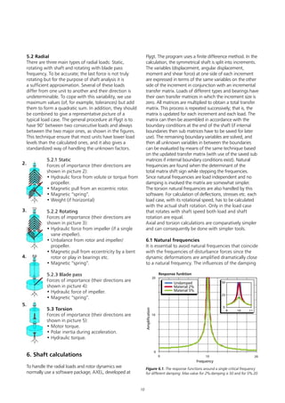
6.5.3 Haigh diagram
In the Haigh diagram in figure (6.5.3) 5 different
curves can be seen.
Cd =
2 • An
10
1 +
2 • An
d
1 +
Cs =
2 • a
An
1 +
1
q =
An
Kr
1 +
1
Kf = 1 + q • (Kt - 1)
Kf =
1
An
•
An
0
σ(r)
σ0
dr
Fatigue, Haigh diagram
400
300
200
100
0
0 100 200 300 400 500 600
Amplitudestress
Mean stress
Unreduced
Reduced
N modified
Yield
Yield reduced
Curve 1, the unreduced curve is drawn from three
points shown in equation (6.5.3.1).
Curve 2, the reduced curve due to load, dimension,
surface and stress concentrations are drawn from
three points shown in equation (6.5.3.2).
Curve 3, the curve modified due to number of cycles
10N
that differ from 10Nm
is drawn from three points
shown in equation (6.5.3.3).
(0 , σu)
(σup , σup)
(σb , 0)
Figure 6.5.3 Haigh diagram
(0 , σu • Cl • Cs / Kf )
(σup • Cl / Kt , σup • Cl • Cd • Cs / Kf )
(σb • Cl / Kt , 0)
(0 , σf • Cl / Kt •
(σup • Cl / Kt , (σf - σup ) • Cl / Kt •
(σb • Cl / Kt , 0)
exp
N
Nm
• log
σup • Cl • Cd • Cs / Kf
σf • Cl / Kt
)
exp
N
Nm
• log
σup • Cl • Cd • Cs / Kf
(σf - σup ) • Cl / Kt
)
σf = σb •
1
1 - Ψ
(6.5.2.1)
(6.5.2.2)
(6.5.2.3)
(6.5.2.4)
(6.5.3.1)
(6.5.3.2)
(6.5.3.3)
15

16. sf
= true ultimate stress
ψ = reduction of area at rupture
An alternative to the true ultimate stress is to use the
ordinary ultimate stress at 100 cycles. This is used in
the FATIGUE program. Another alternative is to use the
factor 0.9 at 1000 cycles.
Curve 4, the unreduced yield curve is drawn from two
points shown in equation (6.5.3.4).
Curve 5, the reduced yield curve (local yield) is drawn
from two points shown in equation (6.5.3.5).
6.5.4 Interpretation
The actual stress plotted in the Haigh diagram should
be in the area of the lower left corner, limited by the
curves. For a ductile material with the mean stress lower
than twice the yield stress and larger than the reduced
yield curve, the actual mean stress may be moved left
to the reduced yield curve. The safety factor is normally
expressed as the ratio of the distance to the limiting curve
and the distance to the actual stress point. If nothing
explicit is mentioned the vertical distances are used.
7. Bearing calculations
The aim of bearing calculations is to estimate how
long a bearing will last within a specified probability.
In the theoretical calculation, failure is defined as
the first sign of pitting, not when the whole bearing
breaks down.
7.1 Time equivalent load
Since there are both dynamic and static radial
reactions that act on a bearing, it is necessary to form
a time equivalent load to use. First, the dynamic parts
are summed. The magnitude of blade pass reaction is
added to the rotating reaction to form the dynamic
part. Then the static and dynamic part is summed as
shown in equation (7.1.1), also included in AXEL.
F = time equivalent force
fm
= calculation factor
Fstat
, Fdyn
= static and dynamic force
At Flygt the bearing lifetime is calculated assuming full
load and a continuously running machine. If different
loads are involved during a run pattern then equation
(7.1.2) is appropriate.
F = time equivalent force
Fi
= force i
Ui
= time fraction of force i
7.2 Equivalent load
The relation between axial and radial force on a bearing
affects the distribution of loads on the different rolling
elements. For example, a purely axial load is to be
shared by all rolling elements, but a purely radial one
acts on fewer rolling elements and is more unevenly
distributed. Conditions like clearance and mounting
also affect this load. Normally, simple formulas from the
bearing manufacturer, as in equation (7.2), can be used,
although this is normally handled by bearing calculation
programs. See figure (7.3.1)
P = equivalent dynamic load
X,Y = constants for different bearing types and
different load cases
Fr ,
Fy
= radial and axial force
7.3 ISO standard 281
The ISO standard for bearing calculation has been
modified in some steps since the equation (7.3.1) was
introduced in 1962. The base for that formula was the
work of Weibull, a theory of statistical endurance of
metallic materials in 1936, and the work of Lundeberg
and Palmgren, who calculated the stresses in the
volume affected by the Herzian pressure in 1947. In
1977 the factors for reliability, material and lubrication
(a1
, a2
and a3
) was added to enhance the calculation.
The latest enhancements are the introduction of fatigue
load limit and influence of contamination that form the
factor am
to be used in lifetime calculations. This work
by mainly Ioannidis has introduced two improvements:
A fatigue stress limit and more accurately and detailed
calculations of the stressed volume with local stresses
which thereby include influence of surface error and
contaminations. Reference 5 gives the details and
reference 6 gives a “popular” version.
7.3.1 Basic formula
The formula for nominal life at 10% probability of
failure is:
F = fm • (Fstat - Fdyn )
fm =
Max (Fstat , Fdyn )
(Fstat + Fdyn )
3
4
• - 0.5
2
F =
∑ Ft
3
• Ui
∑ Ui
1
/3
P = X • Fr - Y • Fy
L10 =
C
P
p
L10h =
10
6
60 • n
• L10
(0 , σs )
(σs , 0)
(0 , σs • Cl / Kt )
(σs • Cl / Kt , 0)
(6.5.3.4)
(6.5.3.5)
(7.1.1)
(7.1.2)
(7.2)
(7.3.1)
16

17. L10
= nominal life in rev×106
L10h
= nominal lifetime in hours
P = equivalent dynamic load
C = dynamic load rating
p = exponent; 3 for ball bearings and 10/3 for roller
bearings
n = rotational speed, rev/min
The value of C is
provided by the bearing
manufacturer and
achieved through a lot
of testing. A normal
calculation from SKF
online catalogue is
shown in figure (7.3.1)
7.3.2 Reliability
The reliability factor is 1
for 90% reliability and
it should be lowered
for higher reliability:
Figure (7.3.2) give values
that follow a Weibull
distribution with a
Weibull slope of 1.5 as adopted by ISO.
L10h
= nominal lifetime in hours
Lnh
= nominal lifetime with altered reliability n
according to a1
a1
= reliability factor
7.3.3 Viscosity
The required lubricant has to have sufficient viscosity
in order to separate the rolling surfaces and distribute
the pressure to achieve acceptable stress levels. The
diagram in figure (7.3.3.1) gives the required viscosity
as a function of bearing size and speed.
The viscosity is highly temperature dependent and the
viscosity at the running temperature is needed. The
viscosity of the grease is normally given at 40 °C and
with normal viscosity index the use of diagrams, as in
figure (7.3.3.2) can provide the correct figure.
Figure 7.3.1. An online calcu-
lation from SKF.
Reliability factor
3.5
3
2.5
2
1.5
1
0.5
0
50 55 60 65 70 75 80 85 90 95 100
a1Factor Reliability %
Figure 7.3.2. Reliability factor a1
. Ln
= a1
• L10
Lnh = a1 • L10
Figure 7.3.3.1. Required viscosity ν1
as a funktion of speed and
mean diameter of the bearing. (SKF)
(7.3.2)
17

18. If the grease also has data for another temperature,
normally 100 °C, the viscosity at a given temperature
can be calculated as shown in equation (7.3.3.1) with
a loglog to log linearization.
T1, T2, T3 = temperatures in °C with ...
νT
, νT1
, νT2
= ... corresponding viscosity
T0
= 273.15
With the required viscosity and the actual viscosity the
viscosity relation in equation (7.3.3.2) can be obtained
for further use in lifetime calculations.
κ = viscosity ratio
ν1
= required viscosity
ν = actual viscosity
7.3.4 Contamination & fatigue load limit
The contamination degree is tricky to estimate. The
guideline from SKF is shown in table (7.3.4). The
pregreased bearing in Flygt´s products, with their well
protected surrounding, have a contamination factor of
0.7. If not pregreased this value is 0.5.
When loads, lubricant and environmental
considerations have been done there is time to get the
adjustment factor to get the calculated lifetime of a
bearing according to equation (7.3.4).
L10mh
= lifetime in hours
L10h
= nominal lifetime in hours
am
= adjustment factor
k = viscosity ratio
ηc
= contamination factor
P = equivalent dynamic load
Pu
= fatigue load limit
The adjustment factor is achieved from diagrams,
such as the one shown in figure (7.3.4.1), for different
bearing types. The fatigue load limit is provided by the
bearing manufacturer.
Figure 7.3.3.2. Viscosity - temperature relation for different ISO
grade i.e viscosities.
xf (T) = log (T0 - T)
yf (ν) = log (log (ν
2
))
a =
yf (νT2 ) - yf (νT1 )
xf (T2) - xf (T1)
b = yf (νT1) - a • xf (T1)
yf (νT ) = a • xf (T) + b
κ =
ν
ν1
Condition
Very clean
Debris size of the order of the lubricant thickness
Clean
Bearings greased for life and sealed
Normal
Greased for life and shielded
Contaminated
Bearing without seals; particles from surroundings
Heavily contaminated
Intruding fluids and particles, extreme contamination
ηc
1
0.8 - 0.9
0.5 - 0.8
0.5 - 0.1
0
Table 7.3.4. Contamination factor ηc
L10mh = am • L10h
am = f
Pu
P
κ , ηc •
(7.3.3.1)
(7.3.3.2)
(7.3.4)
18

19. Environment: If water or dirt can penetrate the
bearing, the predicted lifetime should be lowered
dramatically: if, on the other hand, the environment is
extremely clean and no exchange with the outer world
takes place, the lifetime can be prolonged (tf
= tf
×2).
7.5 Practical life
The calculated lifetime, although correctly done, is just
one part in estimating the practical life of a bearing.
Moderately loaded bearings may work for a long
time even though signs of fatigue have appeared.
Matters like wear and all the failure causes mentioned
in section 2.3 shall also be considered. A too long a
calculated lifetime can even shorten the practical life
of a bearing. The goal for a Flygt bearing to meet is:
ITT Flygts bearings shall guarantee a service
interval of 50 000 hours and be seen “as
trouble free as a bolt”.
In product development we may also use x-ray
diffraction to analyze bearings exposed to real loads in
a field test. The analysis gives information of loading
and remaining lifetime and thereby enhances lifetime
estimations.
Figure 7.3.4.1. Adjustment factor am from SKF. Variables described
in equation (7.3.4)
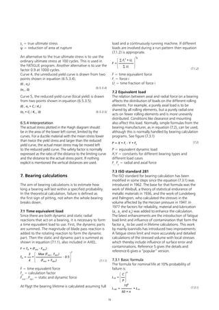
Figure 7.4. Time to relubrication (SKF) T y-axis is operating hours
and the x-axis is the product of speed [rpm], bearing mean diameter
[mm] and a factor 1 for normal ball bearings and ,5 for normal roller
bearings without axial load.
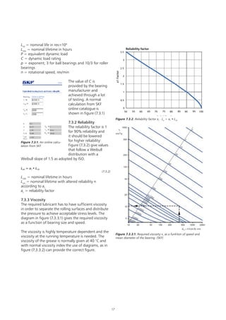
The calculation can be
made by hand with the
help of diagrams but it
is much easier to use the
online program available,
shown in figure (7.3.4.2)
7.4 Lubrication life
The preceding
information naturally
depends on a proper
lubrication which itself
has a specific lifetime.
The lifetime of a grease
lubrication may be far shorter than the lifetime of
a bearing. Some rules together with the diagram in
Figure (7.4) (SKF) provide a rough estimation of the
lifetime of the lubrication. The rules in short (tf
is
lifetime in operating hours):
• If 90% reliability instead of 99%: tf
= tf
×2
• For vertical mounting: tf
= tf
/2
• For every 15°C above 70°C: tf
= tf
/2
• For lower temperatures maximum: tf
= tf
×2
• For synthetic grease above 70°C: tf
= tf
×4
• For synthetic grease below 70°C: tf
= tf
×3
Figure 7.3.4.2. An online
calculation from SKF.
19

20. 7.5.1 Wear
Particles do not only create high stresses in the bearing
and lower the calculated lifetime, they may also cause
wear, another reason for cleanliness of bearings and
their lubrication. The wear rate depends mainly on the
particle concentration, particle size, particle hardness
and sliding.
7.5.2 Lubrication
Lubrication properties are of great importance and
Flygt continuously try to get the best lubrication
for our products. One should note that grease are
perishables and one test Flygt perform to compare
different greases in this respect is heat tests at 140 °C.
This test and others, as well as test from lubricant and
bearing suppliers, give the base from which we predict
lubricant lifetime.
8. Safety factors
To determine the appropriate safety factor to use
there are a lot of considerations to take into account,
type of failure, accuracy in calculations, acceptance
level of failure etc. This can be structured as a set of
factors that can be multiplied to form a safety factor
as shown below:
• Demands 1. Factor for failure probability is 1 if less
serious (failure probability of 10-3
), 1.1 if serious
(failure probability of 10-4
) and 1.2 if very serious
(failure probability of 10-5
).
• Demands 2. Factor for control of calculation,
material, manufacturing and use is 1 if rigorous
control, 1.05 if normal and 1.1 if low degree of
control.
• Load. Factor for load is 1 if maximum values are
used, loads with limitations or fixed load with no
variations. For other conditions, an estimation of the
loads probability has to be done.
• Resistance 1. Factor for material is 1 if guarantied
minimum values or probability of lower values
are less than 10-3
. 1.1 to 1.3 if normal distribution
and average values of ultimate stress, yield stress
and crack propagation values. 1.3 to 1.7 if normal
distribution and average values of fatigue data for
infinite life.
• Resistance 2. Factor for calculation method is 1
if worst case calculation. 1.1 to 1.2 if handbook
formulas or FEA. It is larger than 1.2 if less accurate
methods are used.
• Resistance 3. Factor for criteria is 1 if plastic
deformation or non-brittle failure, if brittle failures
and one-directional stress, if fatigue and infinite
life or if fatigue and constant amplitude at one-
directional stress. 1.1 if brittle failure and multi-
directional stress, if fatigue and limited life or if
fatigue and multi-directional stress. 2 if fatigue
and several different load cases. Time independent
deformation gives a factor of 1, time dependent
deformations 1.1 to 2.
The figures above are given as guidance. If the
probability distribution of the factors above is known,
then a more sophisticated analysis may be performed.
This is, however, normally not the case. The final
safety factor is formed by multiplying the two demand
factors, the load factor and the three resistance
factors.
If a component is tested, like bearings, then the values
obtained from tests are the one to use. This type of
endurance tests is normally not possible to perform,
especially not for components produced in a low
number.
9. Conclusions
When analyzing a rotating system there are many
calculations involved and a lot of assumptions made.
This publication shows how Flygt performs this and
what methods Flygt consider to be the most suitable.
In order to compare predictions of bearing life, safety
levels of different failures etc it is necessary to know
how they have been achieved.
The amount of data needed (and generated) to get
results from one duty point of one combination of
drive unit and hydraulic part is huge. For the entire
pump curve, even more is needed. Consequently, it is
impossible to analyze all combinations of all impellers/
propellers, volutes, drive units and running conditions.
What finally counts is the performance of the product,
not a good figure of some kind. Especially since there
are a lot of failure conditions that are unpredictable
by calculations. Nevertheless, accurate analyzes are
necessary to compare different designs and to create a
robust product that fulfils the customers´ demands.
20

21. References
1. ITT Flygt 892933 CT-design.
Design recommendations for pumping stations with
dry installed submersible pumps.
2. Gert Hallgren
Thermal Analysis of Electrical Pump Motors.
The ITT Flygt Scientific Impeller No. 5, p56-62 (1998)
3. Per Strinning
A computerized trial and error technique for
impeller design.
The ITT Flygt Scientific Impeller No. 3, p19-27 (1995)
4. Thomas Börjesson
Time accurate simulation of a centrifugal pump.
The ITT Flygt Scientific Impeller No. 6, p21-30 (1998)
5. Ioannides E., Harris T.A.
A new fatigue life model for rolling contacts.
Trans ASME JoT, Vol 107 p367-378 (1985)
6. Ioannides E., Bergling G, Gabelli A.
The SKF formula for rolling bearing.
SKF magazine Evolution no 1, p25-28 (2001)
7. SKF
General Catalogue
Catalogue 5000E June 2003.
8. Johannes Brändlein, Paul Eschmann,
Ludwig Hasbargen, Karl Wiegand.
Ball and roller bearings, theory, design and application.
Third Edition
John Wileys & Sons Ltd (1999)
21

22. 22

23. 23

24. www.flygt.com
ITT Flygt is the world’s leading manufacturer and supplier of
submersible pumping and mixing solutions. Flygt submersible
pumps, mixers and aeration systems are used in wastewater
plants, process industries and numerous other applications.
Our experience is utilised by engineers, planners and consult-
ants to ensure reliable and cost-effective operation. ITT Flygt
has service and sales facilities in more than 130 countries.
ShaftandBearingsCalculations.02.03.Eng.0,5M.04.04892932