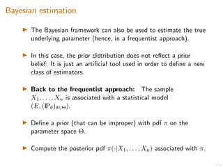
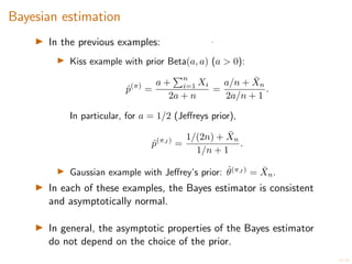
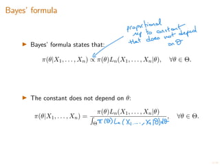
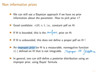
This document discusses Bayesian statistics and compares it to the frequentist approach. The Bayesian approach models uncertainty about parameters through prior distributions, which are updated based on data to obtain posterior distributions. This allows incorporation of prior beliefs. Key concepts covered include Bayes' formula, priors like non-informative and Jeffreys' priors, Bayesian estimation using the posterior mean or maximum a posteriori, and Bayesian confidence regions. Examples of applying Bayesian methods to binomial and normal distributions are provided.

1. 1/20
18.650 – Fundamentals of Statistics
5. Bayesian Statistics

2. 2/20
Goals
So far, we have followed the frequentist approach (cf. meaning of
a confidence interval).
An alternative is the Bayesian approach.
New concepts will come into play:
I prior and posterior distributions
I Bayes’ formula
I Priors: improper, non informative
I Bayesian estimation: posterior mean, Maximum a posteriori
(MAP)
I Bayesian confidence region
In a sense, Bayesian inference amounts to having a likelihood
function Ln(✓) that is weighted by prior knowledge on what ✓
might be. This is useful in many applications.

3. 3/20
The frequentist approach
I Assume a statistical model (E, {IP✓}✓2⇥).
I We assumed that the data X1, . . . , Xn was drawn i.i.d from
IP✓⇤ for some unknown ✓⇤.
I When we used the MLE for example, we looked at all possible
✓ 2 ⇥.
I Before seeing the data we did not prefer a choice of ✓ 2 ⇥
over another.

4. 4/20
The Bayesian approach
I In many practical contexts, we have a belief about ✓⇤
I Using the data, we want to update that belief and transform
it into a belief.

5. 5/20
The kiss example
I Let p be the proportion of couples that turn their head to the
right
I Let X1, . . . , Xn
i.i.d
⇠ Ber(p).
I In the frequentist approach, we estimated p (using the MLE),
we constructed some confidence interval for p, we did
hypothesis testing (e.g., H0 : p = .5 v.s. H1 : p 6= .5).
I Before analyzing the data, we may believe that p is likely to
be close to 1/2.
I The Bayesian approach is a tool to update our prior belief
using the data.

6. 6/20
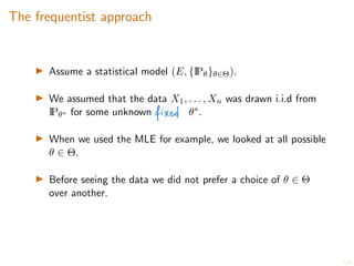
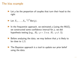
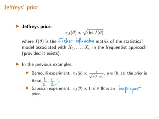
The kiss example
I Our prior belief about p can be quantified:
I E.g., we are 90% sure that p is between .4 and .6, 95% that it
is between .3 and .8, etc...
I Hence, we can model our prior belief using a distribution for
p, as if p was random.
I In reality, the true parameter is not random ! However, the
Bayesian approach is a way of modeling our belief about the
parameter by doing as if it was random.
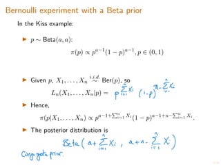
I E.g., p ⇠ Beta(a, b) (Beta distribution. It has pdf
f(x) =
1
K
xa 1
(1 x)b 1
1
I(x 2 [0, 1]), K =
Z 1
0
ta 1
(1 t)b 1
dt
I This distribution is called the

7. 7/20
The kiss example
I In our statistical experiment, X1, . . . , Xn are assumed to be
i.i.d. Bernoulli r.v. with parameter p conditionally on .
I After observing the available sample X1, . . . , Xn, we can
update our belief about p by taking its distribution
conditionally on the data.
I The distribution of p conditionally on the data is called the
I Here, the posterior distribution is
Beta a +
n
X
i=1
Xi, a + n
n
X
i=1
Xi

8. 8/20
Clinical trials
Let us revisit our clinical trial example
I Pharmaceutical companies use hypothesis testing to test if a
new drug is efficient.
I To do so, they administer a drug to a group of patients (test
group) and a placebo to another group (control group).
I We consider testing a drug that is supposed to lower LDL
(low-density lipoprotein), a.k.a ”bad cholesterol” among
patients with a high level of LDL (above 200 mg/dL)

9. 9/20
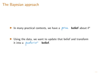
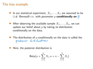
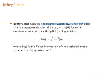
Clinical trials
I Let d > 0 denote the expected decrease of LDL level (in
mg/dL) for a patient that has used the drug.
I Let c > 0 denote the expected decrease of LDL level (in
mg/dL) for a patient that has used the placebo.
Quantity of interest: ✓ := .
In practice we have a prior belief on ✓. For example,
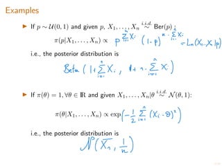
I ✓ ⇠ Unif([100, 200])
I ✓ ⇠ Exp(100)
I ✓ ⇠ N(100, 300),
I . . .

10. 10/20
Prior and posterior
I Consider a probability distribution on a parameter space ⇥
with some pdf ⇡(·): the prior distribution.
I Let X1, . . . , Xn be a sample of n random variables.
I Denote by Ln(·|✓) the joint pdf of X1, . . . , Xn conditionally
on ✓, where ✓ ⇠ ⇡.
I Remark: Ln(X1, . . . , Xn|✓) is the used in the
frequentist approach.
I The conditional distribution of ✓ given X1, . . . , Xn is called
the posterior distribution. Denote by ⇡(·|X1, . . . , Xn) its pdf.

11. 11/20
Bayes’ formula
I Bayes’ formula states that:
⇡(✓|X1, . . . , Xn) / ⇡(✓)Ln(X1, . . . , Xn|✓), 8✓ 2 ⇥.
I The constant does not depend on ✓:
⇡(✓|X1, . . . , Xn) =
⇡(✓)Ln(X1, . . . , Xn|✓)
R
⇥
, 8✓ 2 ⇥.

12. 12/20
Bernoulli experiment with a Beta prior
In the Kiss example:
I p ⇠ Beta(a, a):
⇡(p) / pa 1
(1 p)a 1
, p 2 (0, 1)
I Given p, X1, . . . , Xn
i.i.d.
⇠ Ber(p), so
Ln(X1, . . . , Xn|p) =
I Hence,
⇡(p|X1, . . . , Xn) / pa 1+
Pn
i=1 Xi
(1 p)a 1+n
Pn
i=1 Xi
.
I The posterior distribution is

13. 13/20
Non informative priors
I We can still use a Bayesian approach if we have no prior
information about the parameter. How to pick prior ⇡?
I Good candidate: ⇡(✓) / 1, i.e., constant pdf on ⇥.
I If ⇥ is bounded, this is the prior on ⇥.
I If ⇥ is unbounded, this does not define a proper pdf on ⇥ !
I An improper prior on ⇥ is a measurable, nonnegative function
⇡(·) defined on ⇥ that is not integrable.
I In general, one can still define a posterior distribution using an
improper prior, using Bayes’ formula.

14. 14/20
Examples
I If p ⇠ U(0, 1) and given p, X1, . . . , Xn
i.i.d.
⇠ Ber(p) :
⇡(p|X1, . . . , Xn) /
i.e., the posterior distribution is
I If ⇡(✓) = 1, 8✓ 2 IR and given X1, . . . , Xn|✓
i.i.d.
⇠ N(✓, 1):
⇡(✓|X1, . . . , Xn) / exp
i.e., the posterior distribution is

15. 15/20
Je↵reys’ prior
I Je↵reys prior:
⇡J (✓) /
p
det I(✓)
where I(✓) is the matrix of the statistical
model associated with X1, . . . , Xn in the frequentist approach
(provided it exists).
I In the previous examples:
I Bernoulli experiment: ⇡J (p) / 1
p
p(1 p)
, p 2 (0, 1): the prior is
Beta( , ).
I Gaussian experiment: ⇡J (✓) / 1, ✓ 2 IR is an
prior.

16. 16/20
Je↵reys’ prior
I Je↵reys prior satisfies a reparametrization invariance principle:
If ⌘ is a reparametrization of ✓ (i.e., ⌘ = (✓) for some
one-to-one map ), then the pdf ˜
⇡(·) of ⌘ satisfies:
˜
⇡(⌘) /
q
det ˜
I(⌘),
where ˜
I(⌘) is the Fisher information of the statistical model
parametrized by ⌘ instead of ✓.

17. 17/20
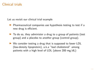
Bayesian confidence regions
I For ↵ 2 (0, 1), a Bayesian confidence region with level ↵ is a
random subset R of the parameter space ⇥, which depends
on the sample X1, . . . , Xn, such that:
IP[✓ 2 R|X1, . . . , Xn] =
I Note that R depends on the prior ⇡(·).
I ”Bayesian confidence region” and ”confidence interval” are
two distinct notions.

18. 18/20
Bayesian estimation
I The Bayesian framework can also be used to estimate the true
underlying parameter (hence, in a frequentist approach).
I In this case, the prior distribution does not reflect a prior
belief: It is just an artificial tool used in order to define a new
class of estimators.
I Back to the frequentist approach: The sample
X1, . . . , Xn is associated with a statistical model
(E, (IP✓)✓2⇥).
I Define a prior (that can be improper) with pdf ⇡ on the
parameter space ⇥.
I Compute the posterior pdf ⇡(·|X1, . . . , Xn) associated with ⇡.

19. 19/20
Bayesian estimation
I Bayes estimator:
ˆ
✓(⇡)
=
This is the posterior mean.
I The Bayesian estimator depends on the choice of the prior
distribution ⇡ (hence the superscript ⇡).
I Another popular choice is the point that maximizes the
posterior distribution, provided it is unique. It is called the
MAP (maximum a posteriori):
ˆ
✓map
= argmax
✓2⇥

20. 20/20
Bayesian estimation
I In the previous examples:
I Kiss example with prior Beta(a, a) (a > 0):
p̂(⇡)
=
a +
Pn
i=1 Xi
2a + n
=
a/n + X̄n
2a/n + 1
.
In particular, for a = 1/2 (Je↵reys prior),
p̂(⇡J )
=
1/(2n) + X̄n
1/n + 1
.
I Gaussian example with Je↵rey’s prior: ˆ
✓(⇡J )
= X̄n.
I In each of these examples, the Bayes estimator is consistent
and asymptotically normal.
I In general, the asymptotic properties of the Bayes estimator
do not depend on the choice of the prior.