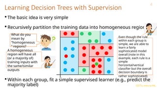
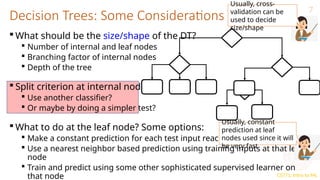
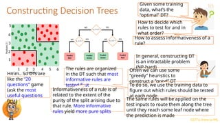
This document provides an overview of decision trees in machine learning, explaining their structure with root, internal, and leaf nodes, and their role in making predictions. It discusses how decision trees are constructed using training data through recursive partitioning into homogeneous regions and the importance of splitting criteria, such as information gain. Additionally, it highlights techniques to avoid overfitting and the efficiency of decision trees compared to other models during prediction.

1. Learning using Decision Trees

2. CS771: Intro to ML
Decision Trees
2
 A Decision Tree (DT) defines a hierarchy of rules to make a
prediction
 Root and internal nodes test rules. Leaf nodes make predictions
 Decision Tree (DT) learning is about learning such a tree from
Body
temp.
Gives
birth
Cold
Non-mammal
Yes No
Non-mammal
Mammal
Root Node
An Internal Node
Warm
A Leaf Node

3. CS771: Intro to ML
A decision tree friendly problem
3
Loan approval prediction

4. CS771: Intro to ML
Learning Decision Trees with Supervision
4
 The basic idea is very simple
 Recursively partition the training data into homogeneous regions
 Within each group, fit a simple supervised learner (e.g., predict the
majority label)
What do you
mean by
“homogeneous
” regions?
A homogeneous
region will have all
(or a majority of)
training inputs with
the same/similar
outputs
Even though the rule
within each group is
simple, we are able to
learn a fairly
sophisticated model
overall (note in this
example, each rule is a
simple
horizontal/vertical
classifier but the overall
decision boundary is
rather sophisticated)

5. CS771: Intro to ML
Decision Trees for Classification
5
1 2 3 4 5 6
1
2
3
4
5
Feature 1 (
𝑥1 >3.5 ?
𝑥2>3 ?
Predict
Red
Predict
Green
𝑥2>2?
Predict
Green
Predict
Red
NO YES
NO YES YES
NO
Test input
DT is very efficient at test time: To predict
the label of a test point, nearest
neighbors will require computing
distances from 48 training inputs. DT
predicts the label by doing just 2 feature-
value comparisons! Way faster!
Remember: Root node
contains all training
inputs
Each leaf node receives a
subset of training inputs

6. CS771: Intro to ML
Decision Trees for Classification: Another Example
6
 Deciding whether to play or not to play Tennis on a Saturday
 Each input (Saturday) has 4 categorical features: Outlook, Temp.,
Humidity, Wind
 A binary classification problem (play vs no-play)
 Below Left: Training data, Below Right: A decision tree constructed
using this data
Example credit: Tom Mitchell

7. CS771: Intro to ML
Decision Trees: Some Considerations 7
 What should be the size/shape of the DT?
 Number of internal and leaf nodes
 Branching factor of internal nodes
 Depth of the tree
 Split criterion at internal nodes
 Use another classifier?
 Or maybe by doing a simpler test?
 What to do at the leaf node? Some options:
 Make a constant prediction for each test input reaching there
 Use a nearest neighbor based prediction using training inputs at that leaf
node
 Train and predict using some other sophisticated supervised learner on
that node
Usually, cross-
validation can be
used to decide
size/shape
Usually, constant
prediction at leaf
nodes used since it will
be very fast

8. CS771: Intro to ML
How to Split at Internal Nodes?
 Recall that each internal node receives a subset of all the training
inputs
 Regardless of the criterion, the split should result in as “pure”
groups as possible
 A pure group means that the majority of the inputs have the same
label/output
8

9. CS771: Intro to ML
Techniques to Split at Internal Nodes
 Each internal node decides which outgoing branch an input should
be sent to
 This decision/split can be done using various ways, e.g.,
 Testing the value of a single feature at a time (such internal node called
“Decision Stump”)
 See here for more details
 Learning a classifier (e.g., LwP or some more sophisticated classifier)
9
DT methods
based on testing
a single feature
at each internal
node are faster
and more
popular (e.g.,
ID3, C4.5 algos)
DT methods based on
learning and using a separate
classifier at each internal node
are less common. But this
approach can be very
powerful and are sometimes
used in some advanced DT
With this approach, all
features and all possible
values of each feature need
to be evaluated in selecting
the feature to be tested at
each internal node
(can be slow but can be
made faster using some
tricks)

10. CS771: Intro to ML
Constructing Decision Trees
10
1 2 3 4 5 6
1
2
3
4
5
Feature 1 (
Feature
2
(
𝑥1 >3.5 ?
𝑥2>3 ?
Predict
Red
Predict
Green
𝑥2> 2?
Predict
Green
Predict
Red
NO YES
NO YES YES
NO
Given some training
data, what’s the
“optimal” DT?
In general, constructing DT
is an intractable problem
(NP-hard)
Often we can use some
“greedy” heuristics to
construct a “good” DT
To do so, we use the training data to
figure out which rules should be tested
at each node
The same rules will be applied on the
test inputs to route them along the tree
until they reach some leaf node where
the prediction is made
How to decide which
rules to test for and in
what order?
The rules are organized
in the DT such that most
informative rules are
tested first
How to assess informativeness of a
rule?
Informativeness of a rule is of
related to the extent of the
purity of the split arising due to
that rule. More informative
rules yield more pure splits
Hmm.. So DTs are
like the “20
questions” game
(ask the most
useful questions
first)

11. CS771: Intro to ML
Decision Tree Construction: An Example
 Let’s consider the playing Tennis example
 Assume each internal node will test the value of one of the features
 Question: Why does it make more sense to test the feature
“outlook” first?
 Answer: Of all the 4 features, it’s the most informative

11

12. CS771: Intro to ML
Entropy and Information Gain
 Assume a set of labelled inputs from C classes, as fraction of class
c inputs
 Entropy of the set is defined as
 Suppose a rule splits into two smaller disjoint sets and
 Reduction in entropy after the split is called information gain
12
Uniform sets (all
classes roughly equally
present) have high
entropy; skewed sets
low
This split has a low IG
(in fact zero IG)
This split has higher
IG

13. CS771: Intro to ML
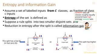
Entropy and Information Gain
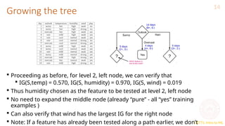
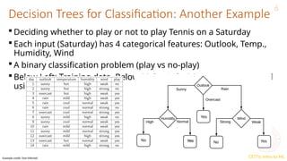
 Let’s use IG based criterion to construct a DT for the Tennis example
 At root node, let’s compute IG of each of the 4 features
 Consider feature “wind”. Root contains all examples S = [9+,5-]
Sweak = [6+, 2−] ⇒ H(Sweak ) = 0.811
Sstrong = [3+, 3−] ⇒ H(Sstrong) = 1
 Likewise, at root: IG(S, outlook) = 0.246, IG(S, humidity) = 0.151, IG(S,temp) =
0.029
 Thus we choose “outlook” feature to be tested at the root node
 Now how to grow the DT, i.e., what to do at the next level? Which feature to
test next?
13
H ( S ) = −(9/14) log 2(9/14) − (5/14) log 2(5/14) = 0.94
= 0.94 8/14 0.811 6/14 1 =
− ∗ − ∗ 0.048

14. CS771: Intro to ML
Growing the tree
 Proceeding as before, for level 2, left node, we can verify that
 IG(S,temp) = 0.570, IG(S, humidity) = 0.970, IG(S, wind) = 0.019
 Thus humidity chosen as the feature to be tested at level 2, left node
 No need to expand the middle node (already “pure” - all “yes” training
examples )
 Can also verify that wind has the largest IG for the right node
 Note: If a feature has already been tested along a path earlier, we don’t
14

15. CS771: Intro to ML
When to stop growing the tree?
 Stop expanding a node further (i.e., make it a leaf node) when
 It consist of all training examples having the same label (the node becomes
“pure”)
 We run out of features to test along the path to that node
 The DT starts to overfit (can be checked by monitoring
the validation set accuracy)
 Important: No need to obsess too much for purity
 It is okay to have a leaf node that is not fully pure, e.g., this
 At test inputs that reach an impure leaf, can predict probability of belonging
to each class (in above example, p(red) = 3/8, p(green) = 5/8), or simply
15
To help prevent the
tree from growing
too much!
OR

16. CS771: Intro to ML
Avoiding Overfitting in DTs
 Desired: a DT that is not too big in size, yet fits the training data reasonably
 Note: An example of a very simple DT is “decision-stump”
 A decision-stump only tests the value of a single feature (or a simple rule)
 Not very powerful in itself but often used in large ensembles of decision
stumps
 Mainly two approaches to prune a complex DT
 Prune while building the tree (stopping early)
 Prune after building the tree (post-pruning)
 Criteria for judging which nodes could potentially be pruned
 Use a validation set (separate from the training set)
 Prune each possible node that doesn’t hurt the accuracy on the
validation set
 Greedily remove the node that improves the validation accuracy the
most
16
Either can be
done using a
validation set

17. CS771: Intro to ML
Decision Trees: Some Comments
 Gini-index defined as can be an alternative to IG
 For DT regression1
, variance in the outputs can be used to assess purity
 When features are real-valued (no finite possible values to try), things are a bit
more tricky
 Can use tests based on thresholding feature values (recall our synthetic
data examples)
 Need to be careful w.r.t. number of threshold points, how fine each range is,
etc.
 More sophisticated decision rules at the internal nodes can also be used
 Basically, need some rule that splits inputs at an internal node into
homogeneous groups
 The rule can even be a machine learning classification algo (e.g., LwP or a
deep learner)
17
man, Leo; Friedman, J. H.; Olshen, R. A.; Stone, C. J. (1984). Classification and regression trees

18. CS771: Intro to ML
An Illustration: DT with Real-Valued Features 18
“Best” (purest possible)
Horizontal Split
“Best”(purest possible)
Vertical Split
Up Down Left Right
Test example
Between the best horizontal
vs best vertical split, the
vertical split is better (purer),
hence we use this rule for the
internal node
his illustration’s credit: Purushottam Kar

19. CS771: Intro to ML
Decision Trees for Regression 19
1 2 3 4 5
4
3
2
1
𝐱
y
𝑥>4 ?
Predict
𝑥2>3 ?
NO YES
NO YES
Predict Predict
Can use any
regression model but
would like a simple
one, so let’s use a
constant prediction
based regression
model
To predict the output for a test point,
nearest neighbors will require computing
distances from 15 training inputs. DT
predicts the label by doing just at most
feature-value comparisons! Way faster!
Another simple
option can be to
predict the
average output of
the training
inputs in this
region

20. CS771: Intro to ML
Decision Trees: A Summary
Some key strengths:
 Simple and easy to interpret
 Nice example of “divide and conquer”
paradigm in machine learning
 Easily handle different types of
features (real, categorical, etc.)
 Very fast at test time
 Multiple DTs can be combined
via ensemble methods: more powerful
(e.g., Decision Forests; will see later)
 Used in several real-world ML applications, e.g., recommender systems,
gaming (Kinect)
Some key weaknesses:
 Learning optimal DT is (NP-hard) intractable. Existing algos mostly greedy
20
1 2 3 4 5 6
1
2
3
4
5
Feature 1 (
Feature
2
(
𝑥1 >3.5 ?
𝑥2>3 ?
Predict
Red
Predict
Green
𝑥2>2?
Predict
Green
Predict
Red
NO YES
NO YES YES
NO
Human-body
pose
estimation
.. thus helping us learn complex
rule as a combination of several
simpler rules