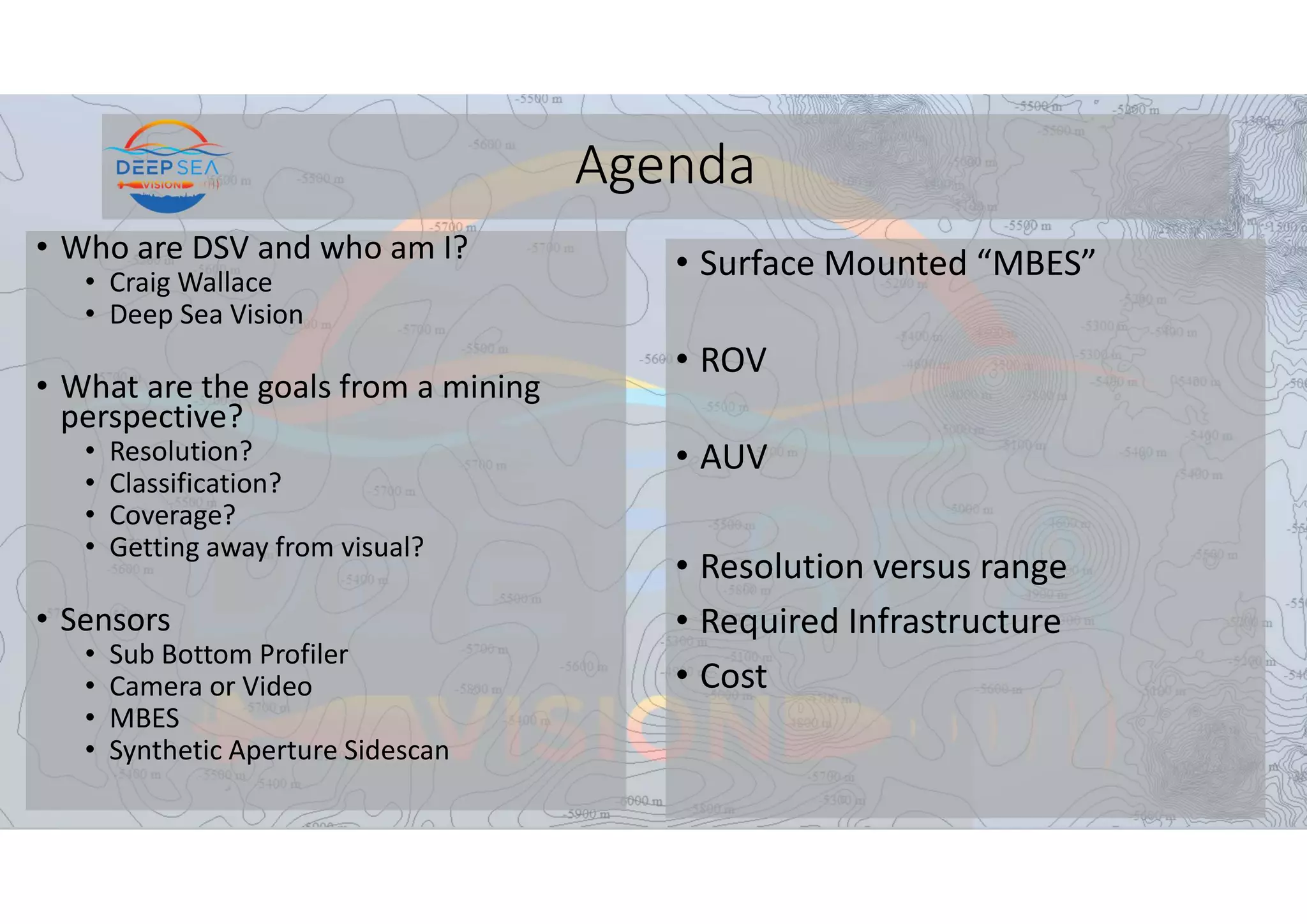
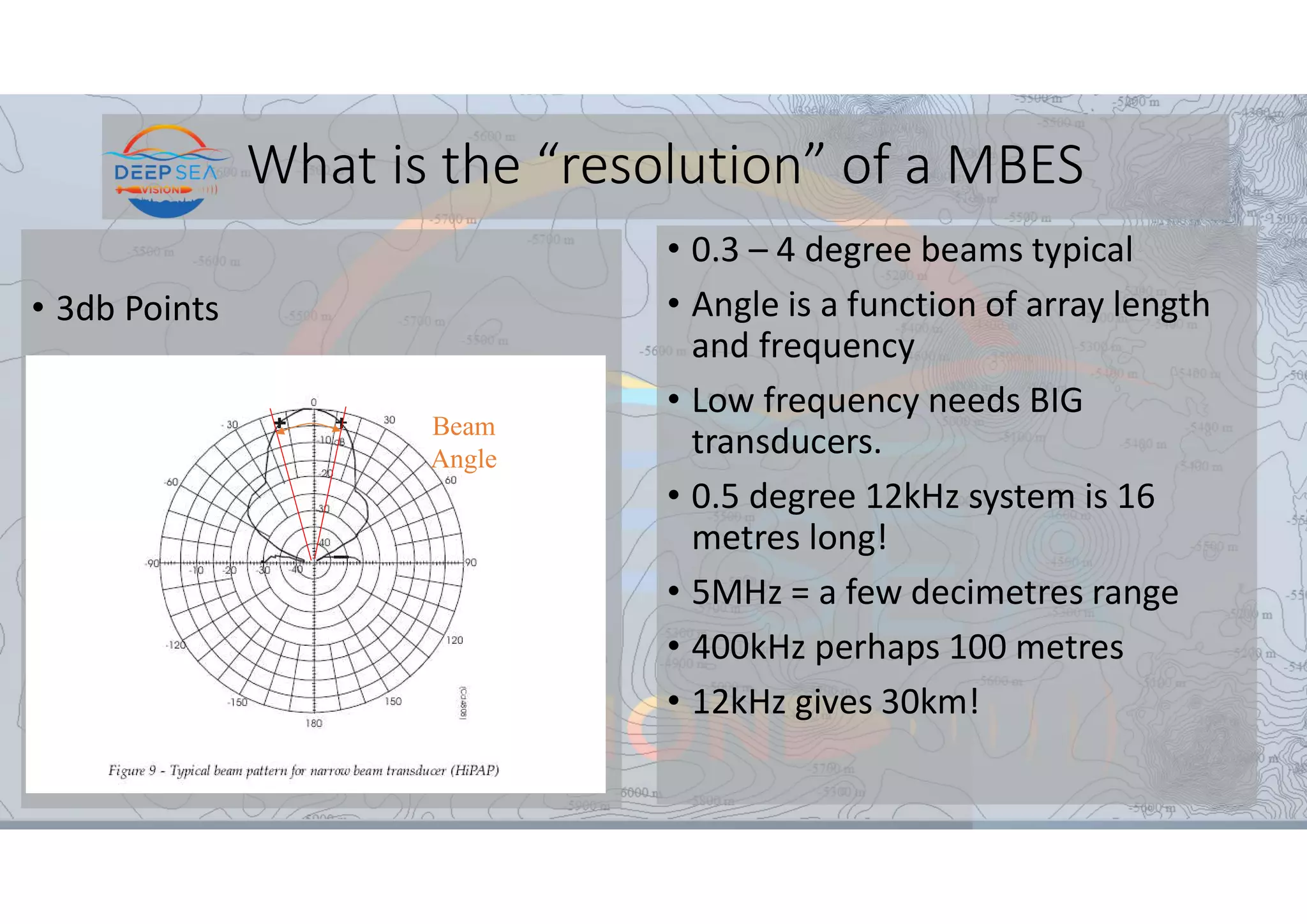
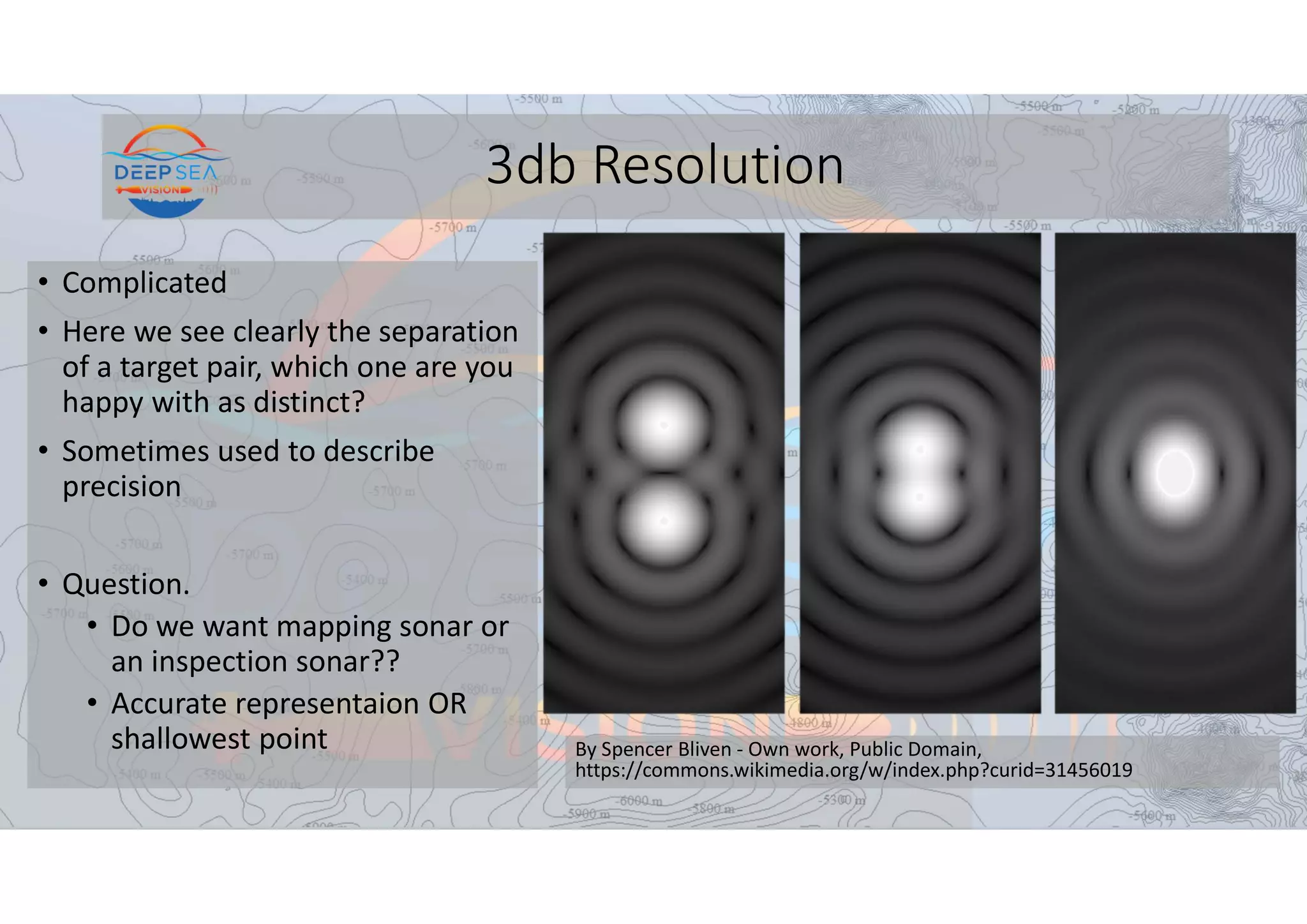
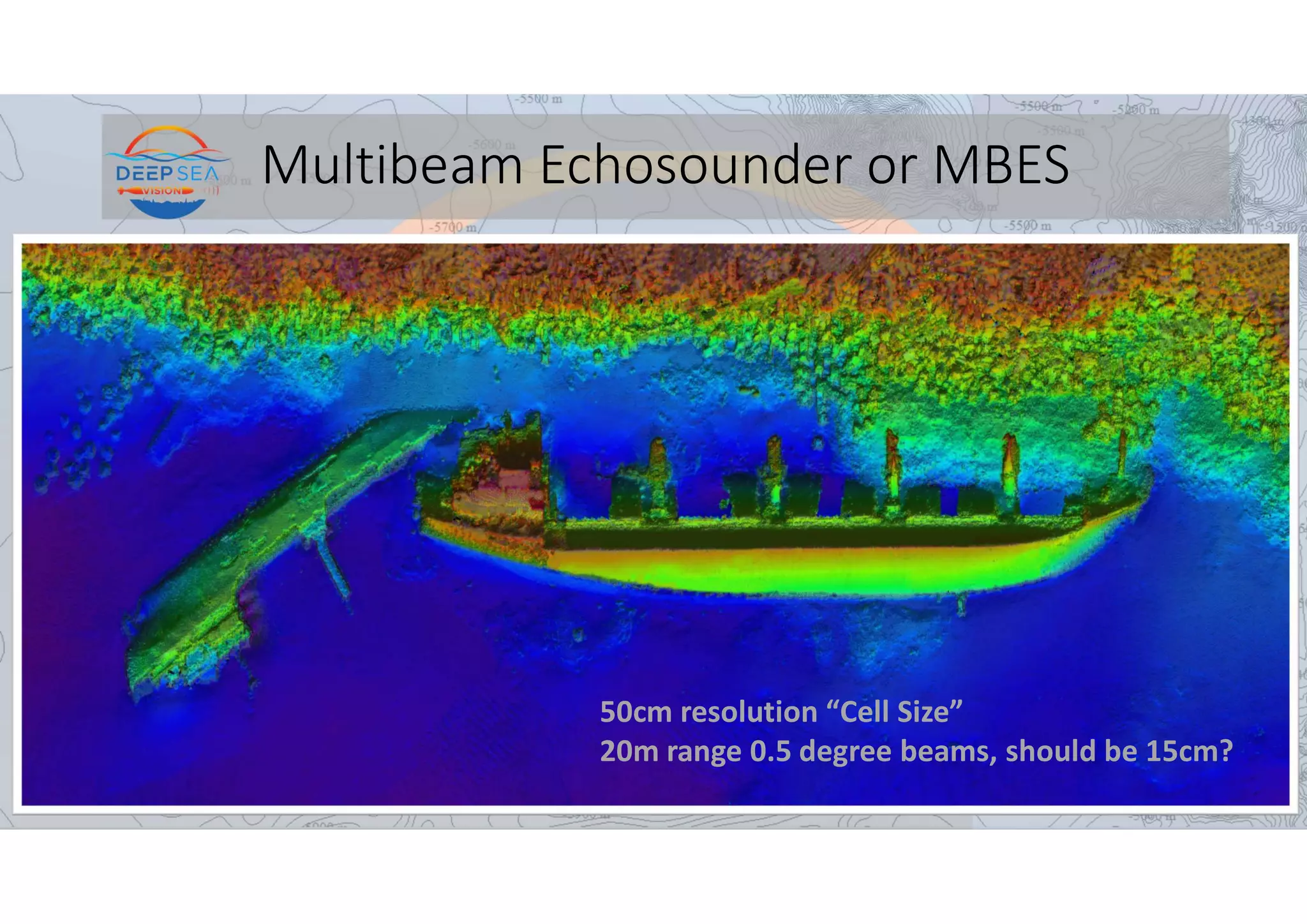
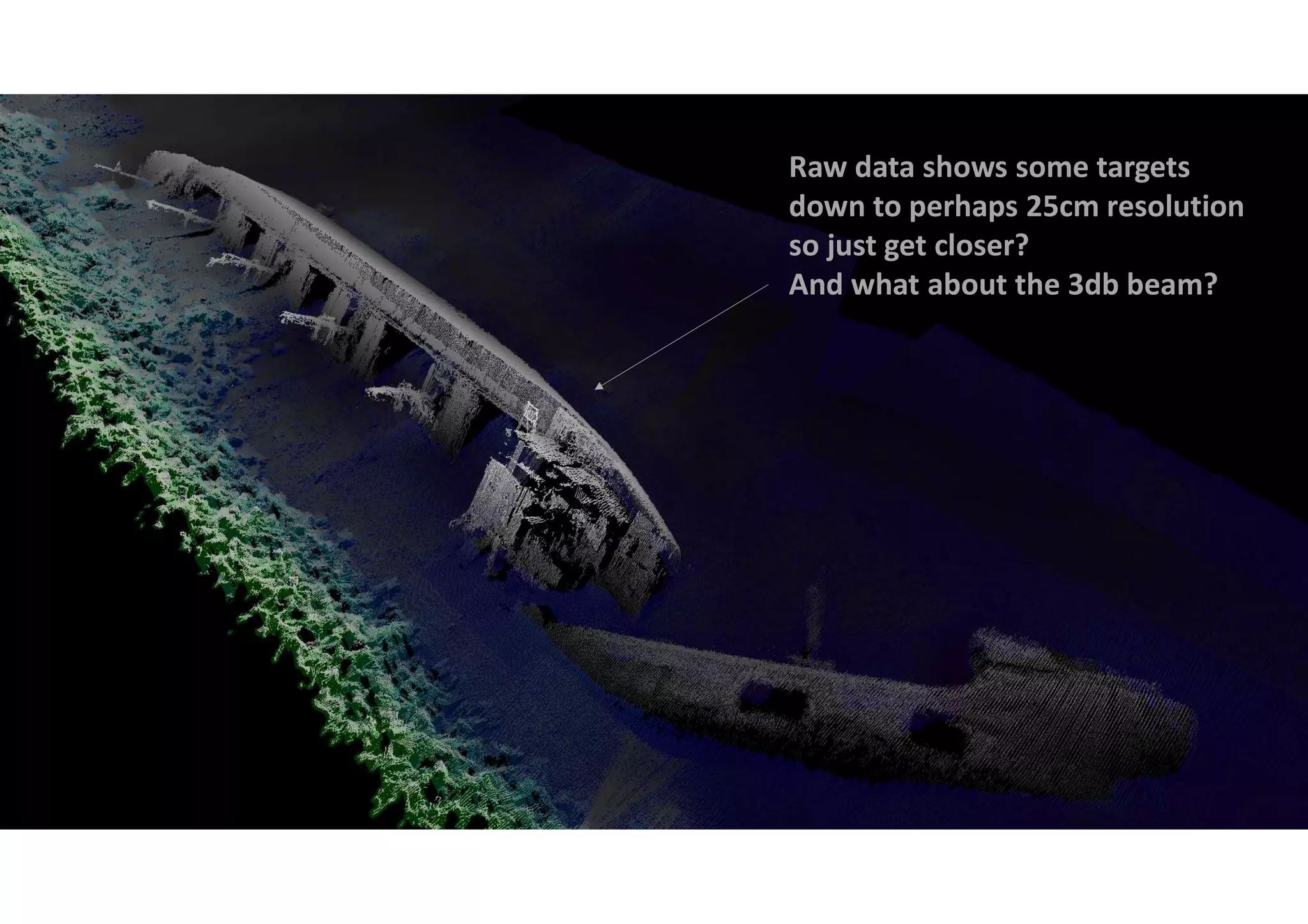
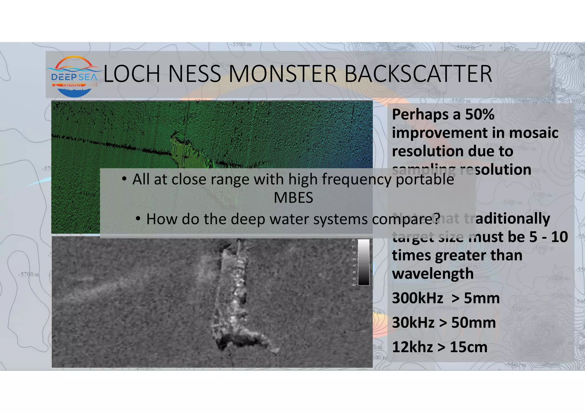
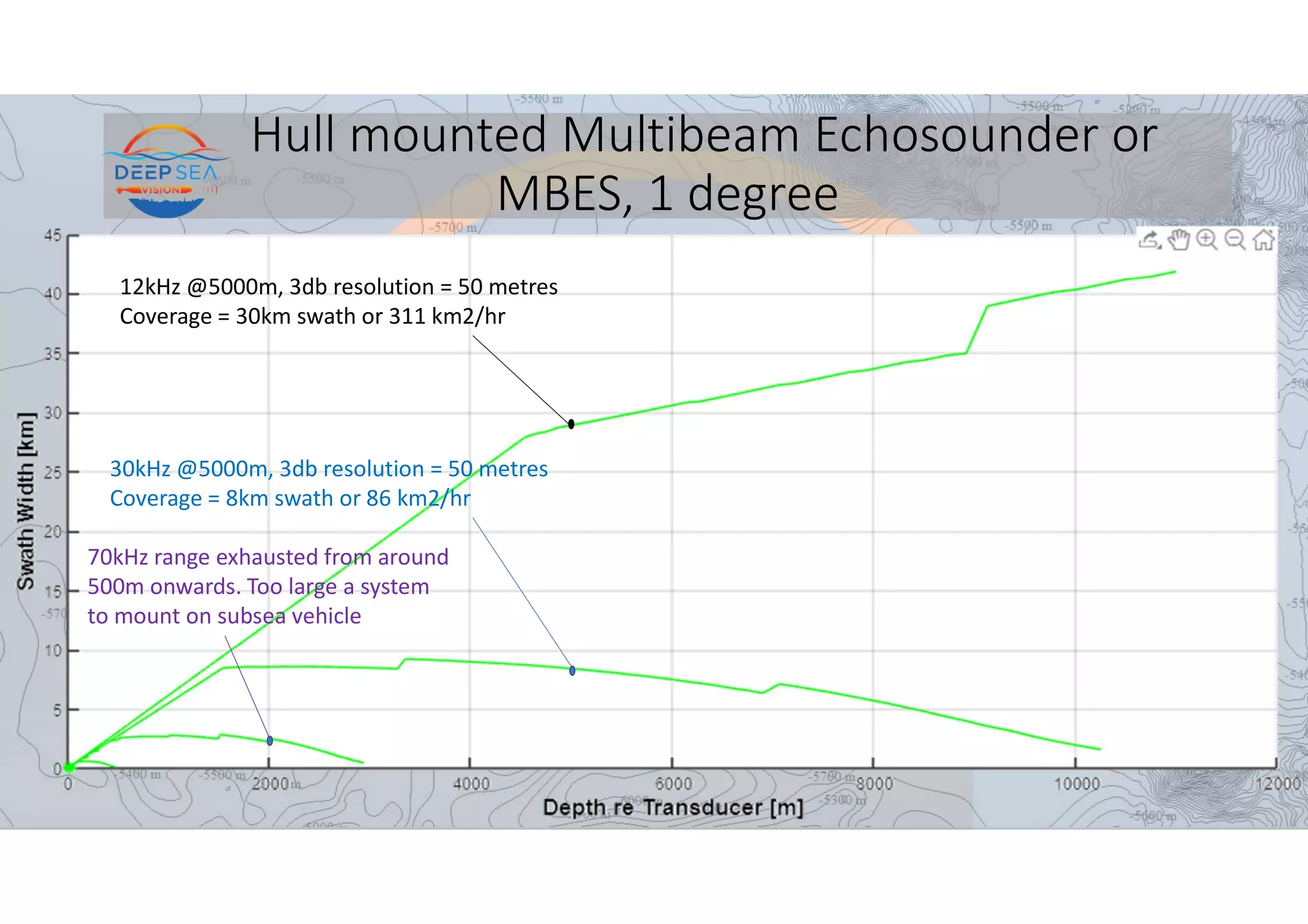
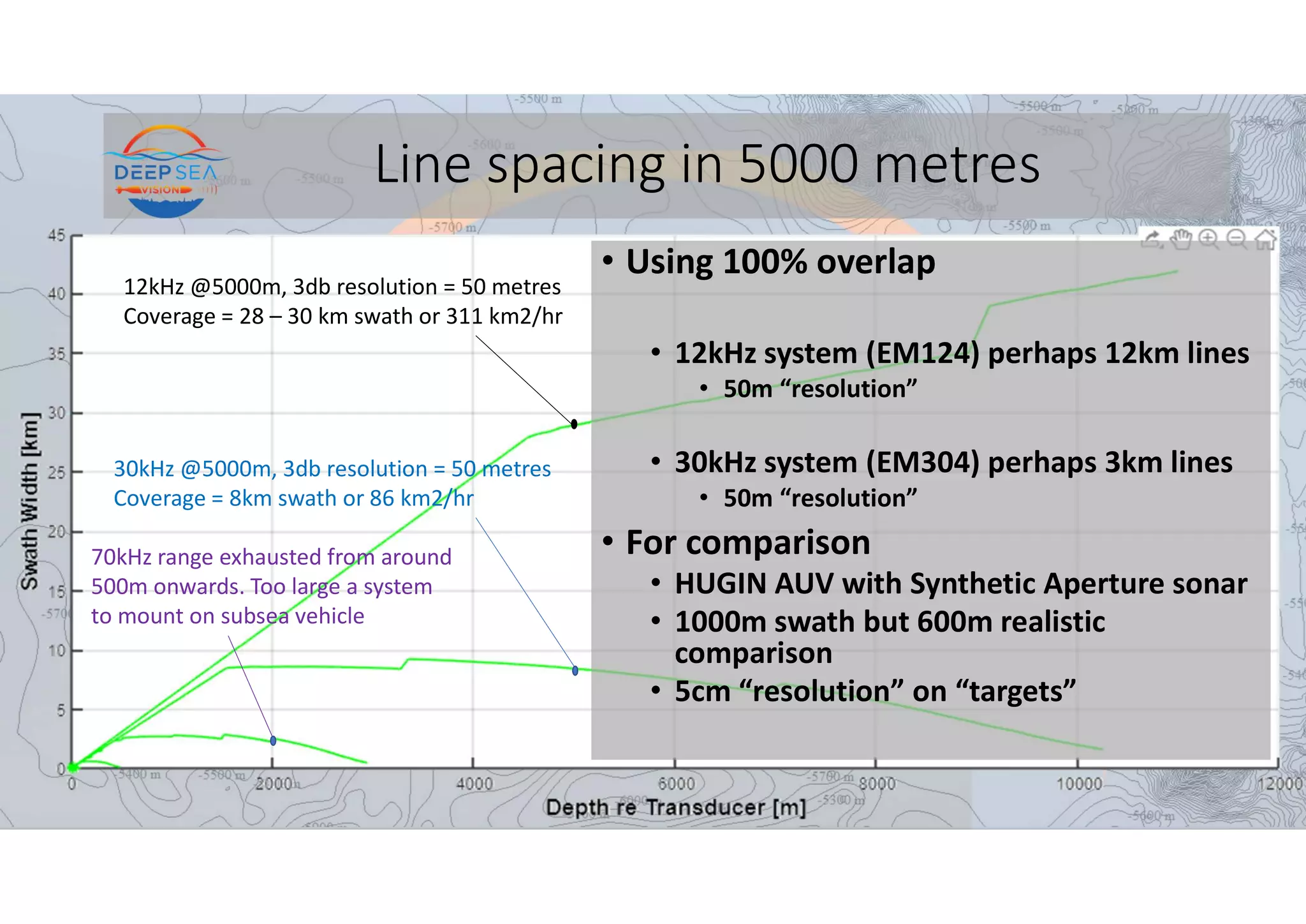
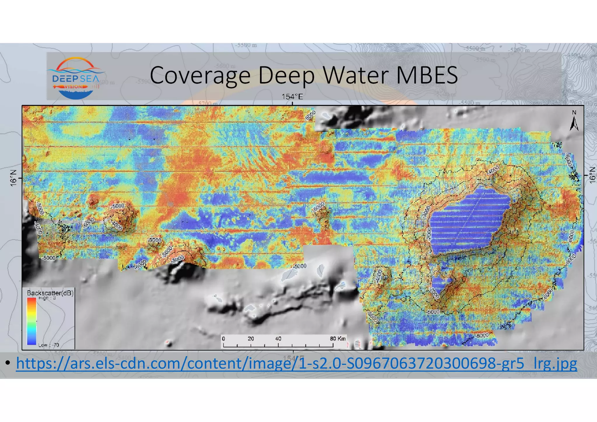
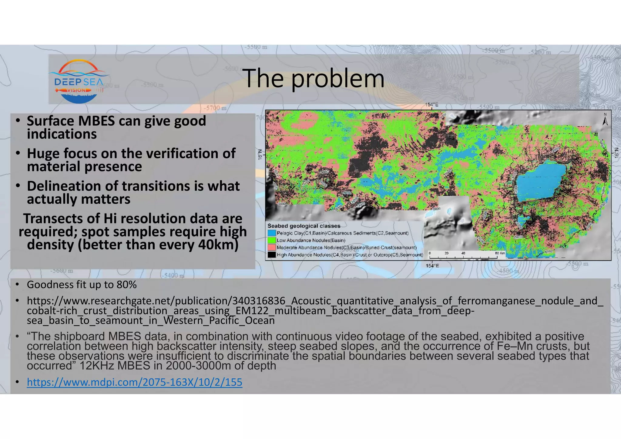
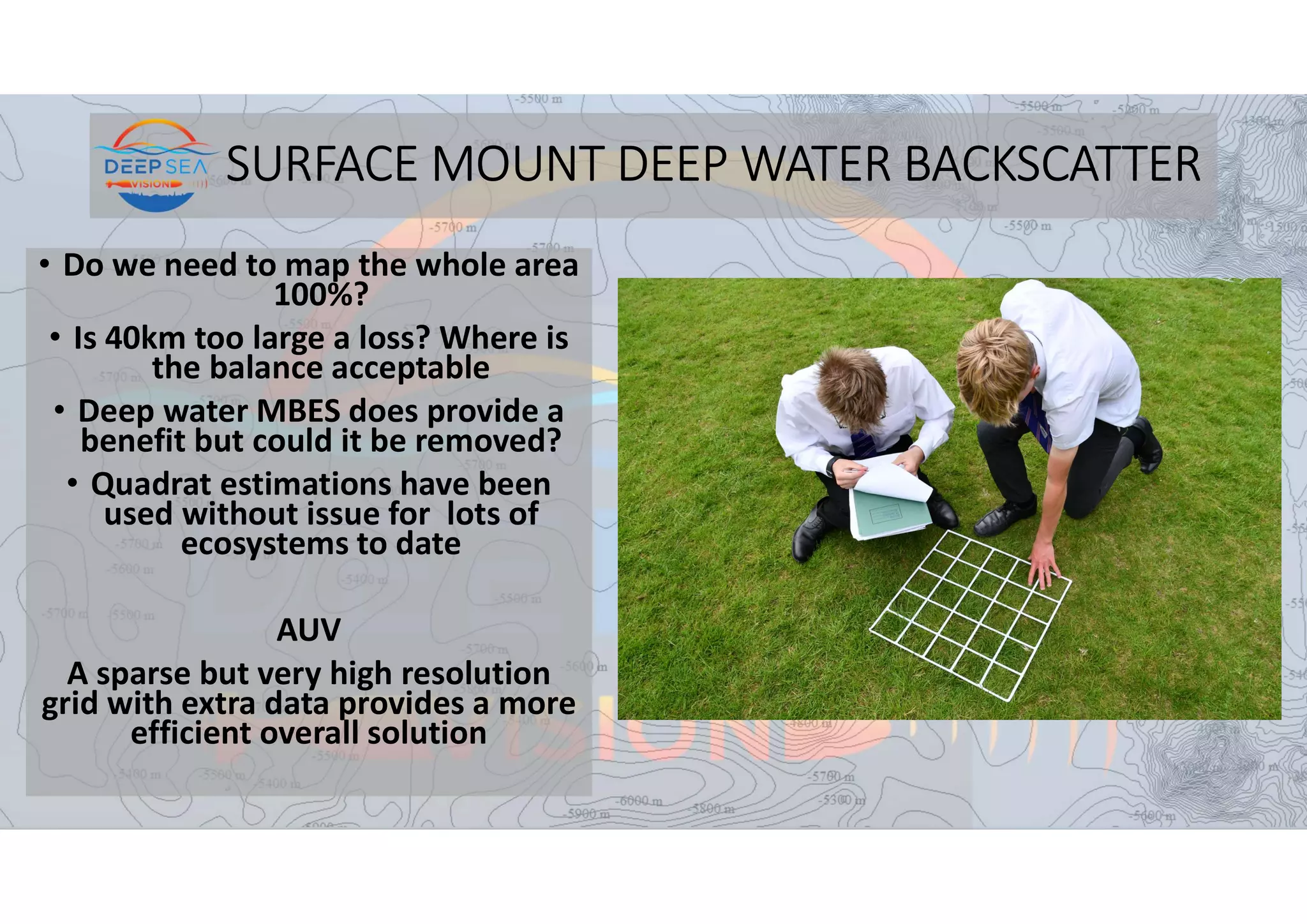
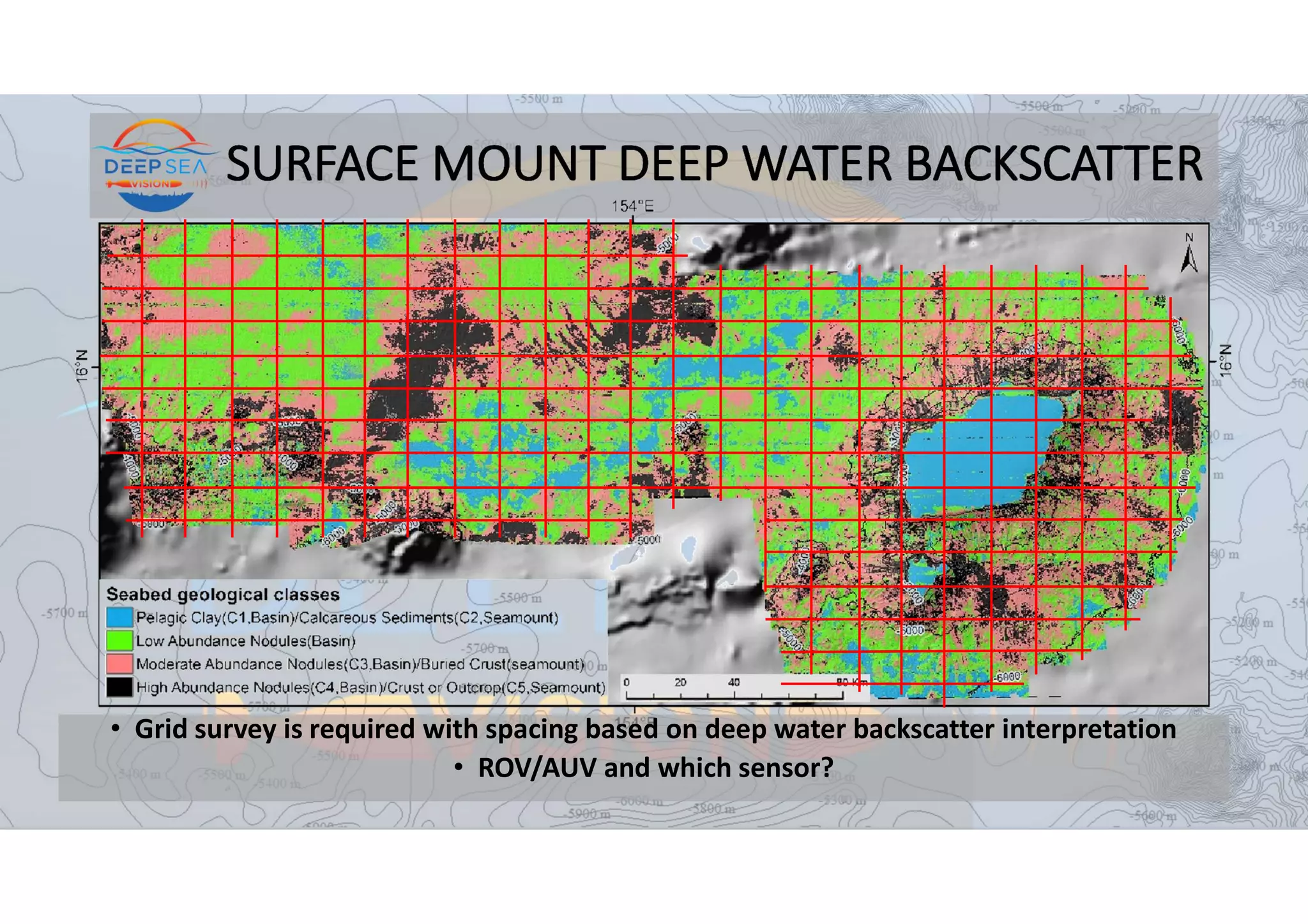
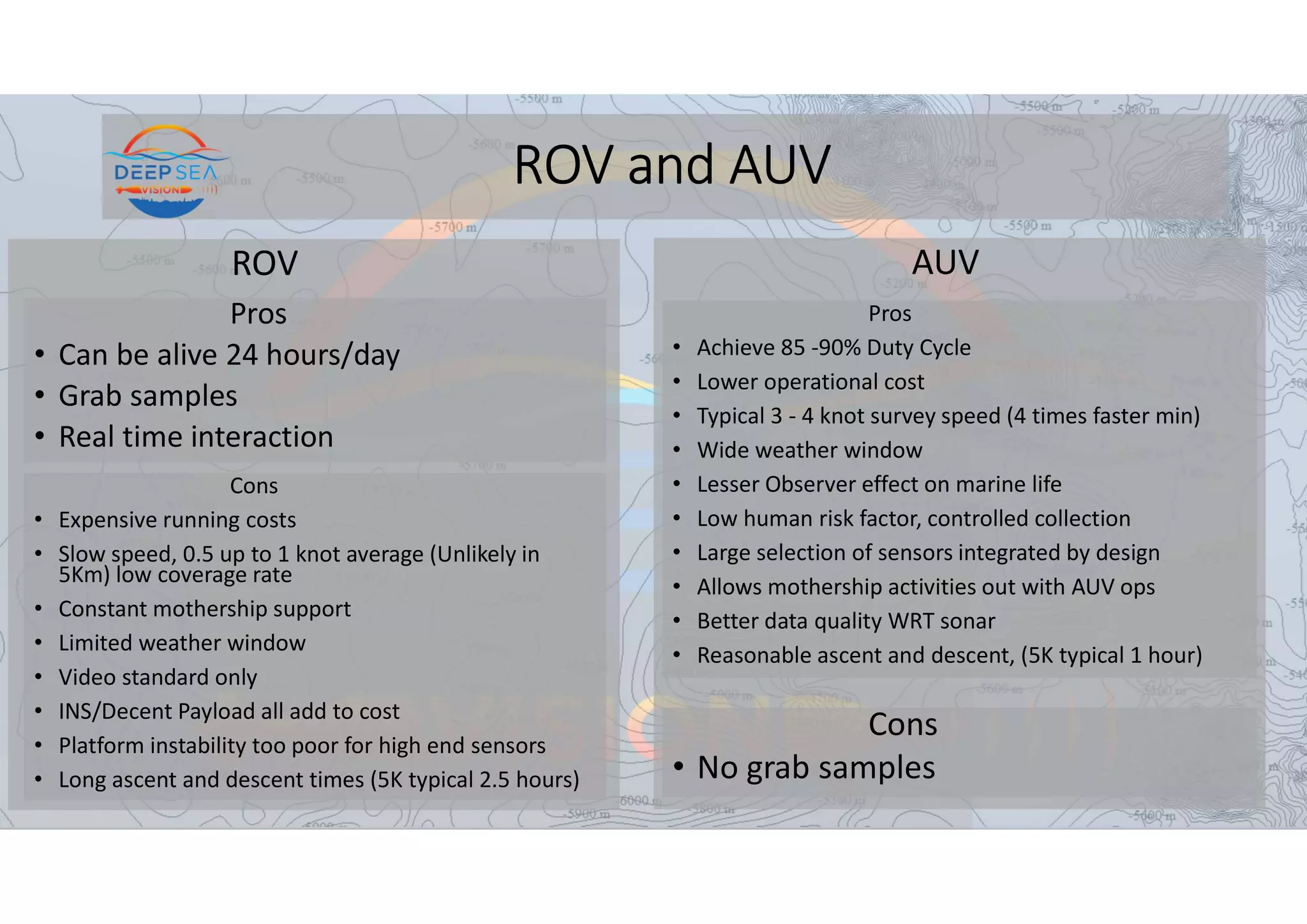
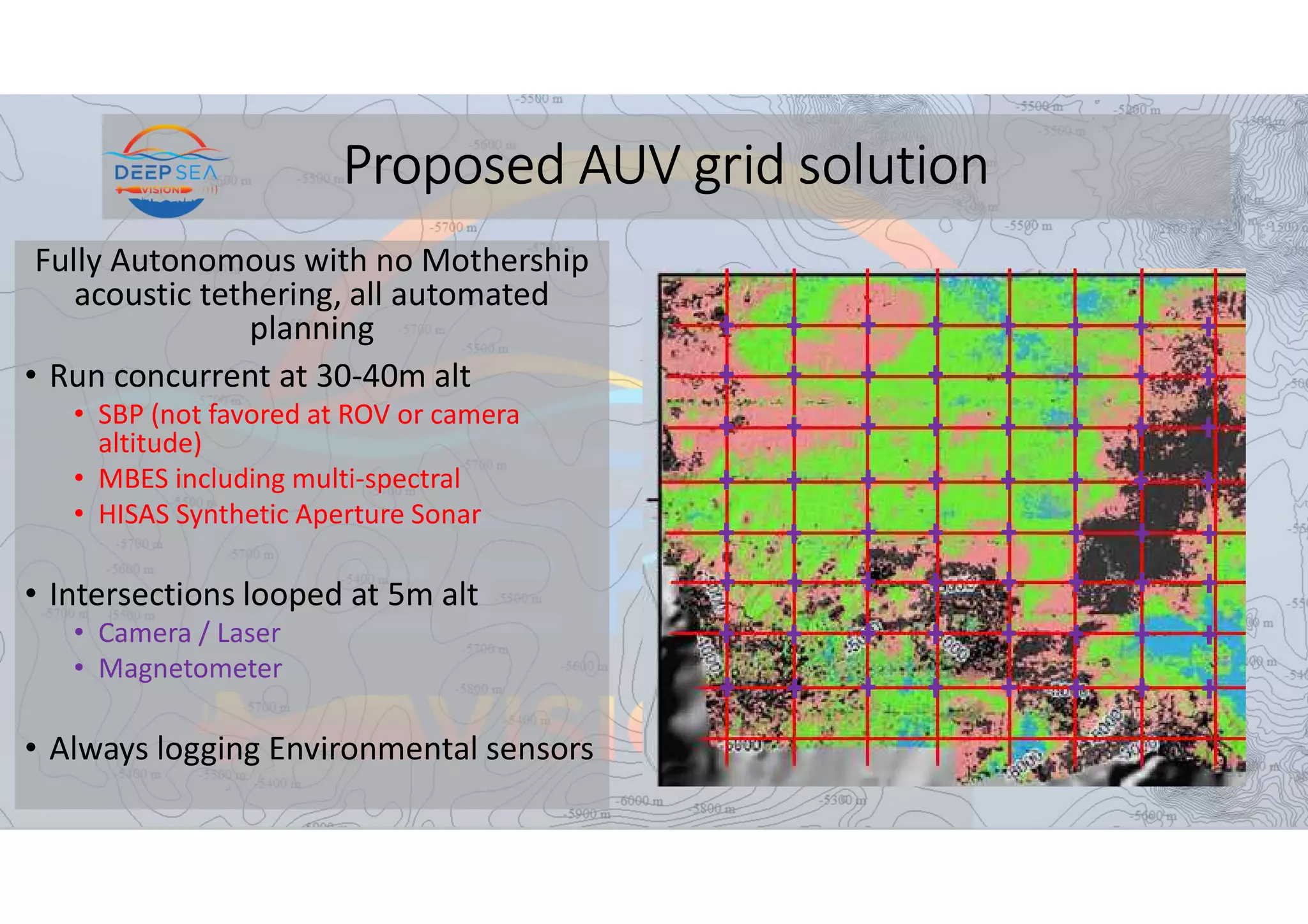
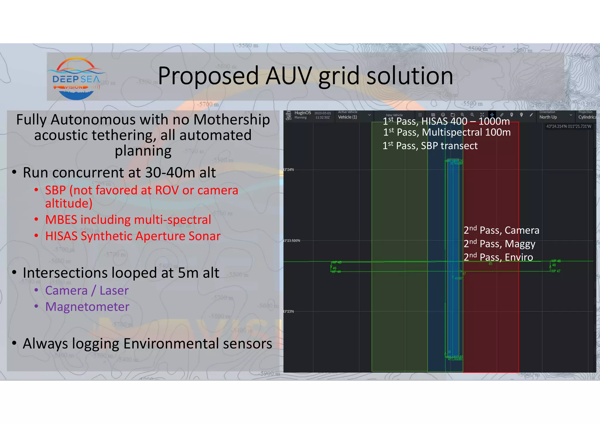
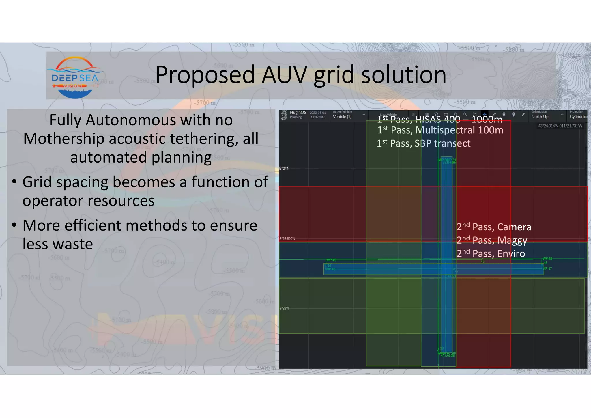
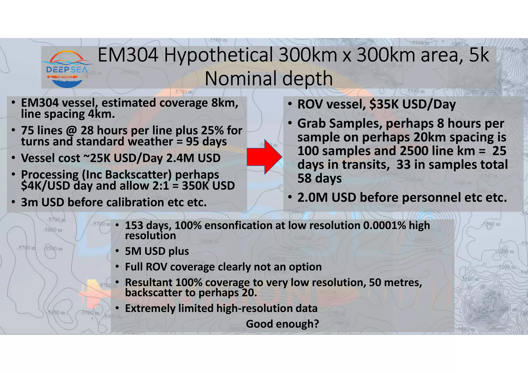
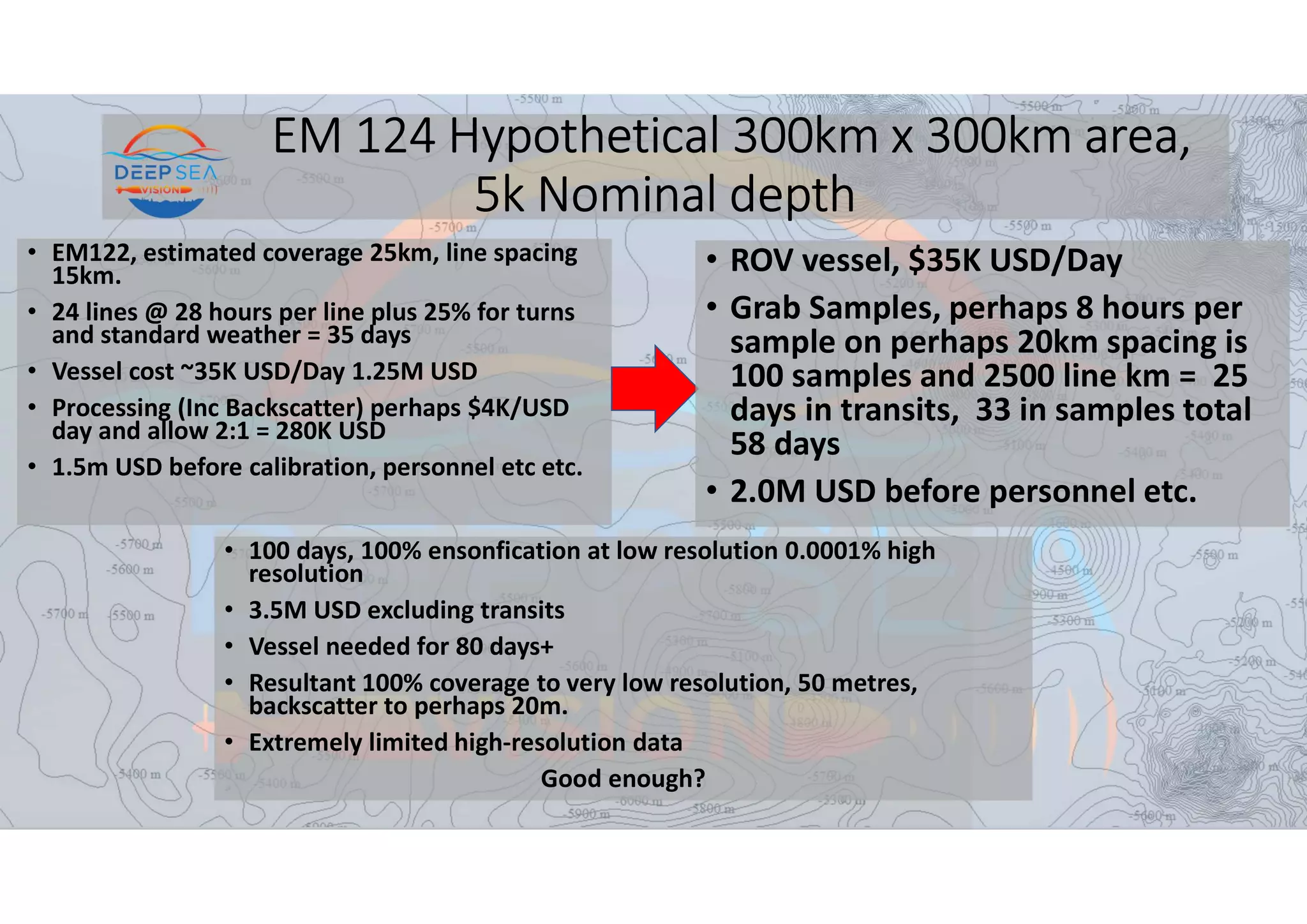
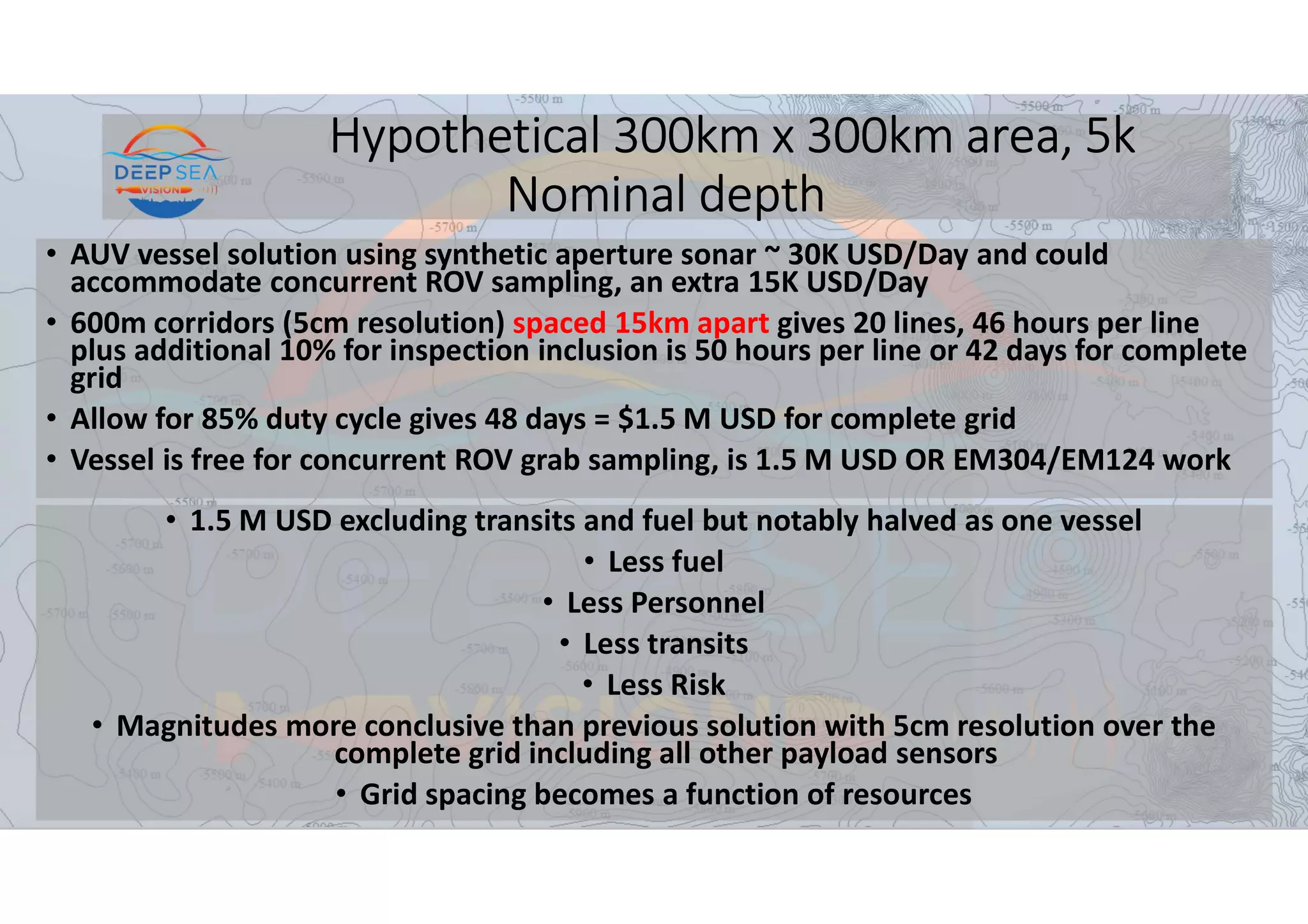
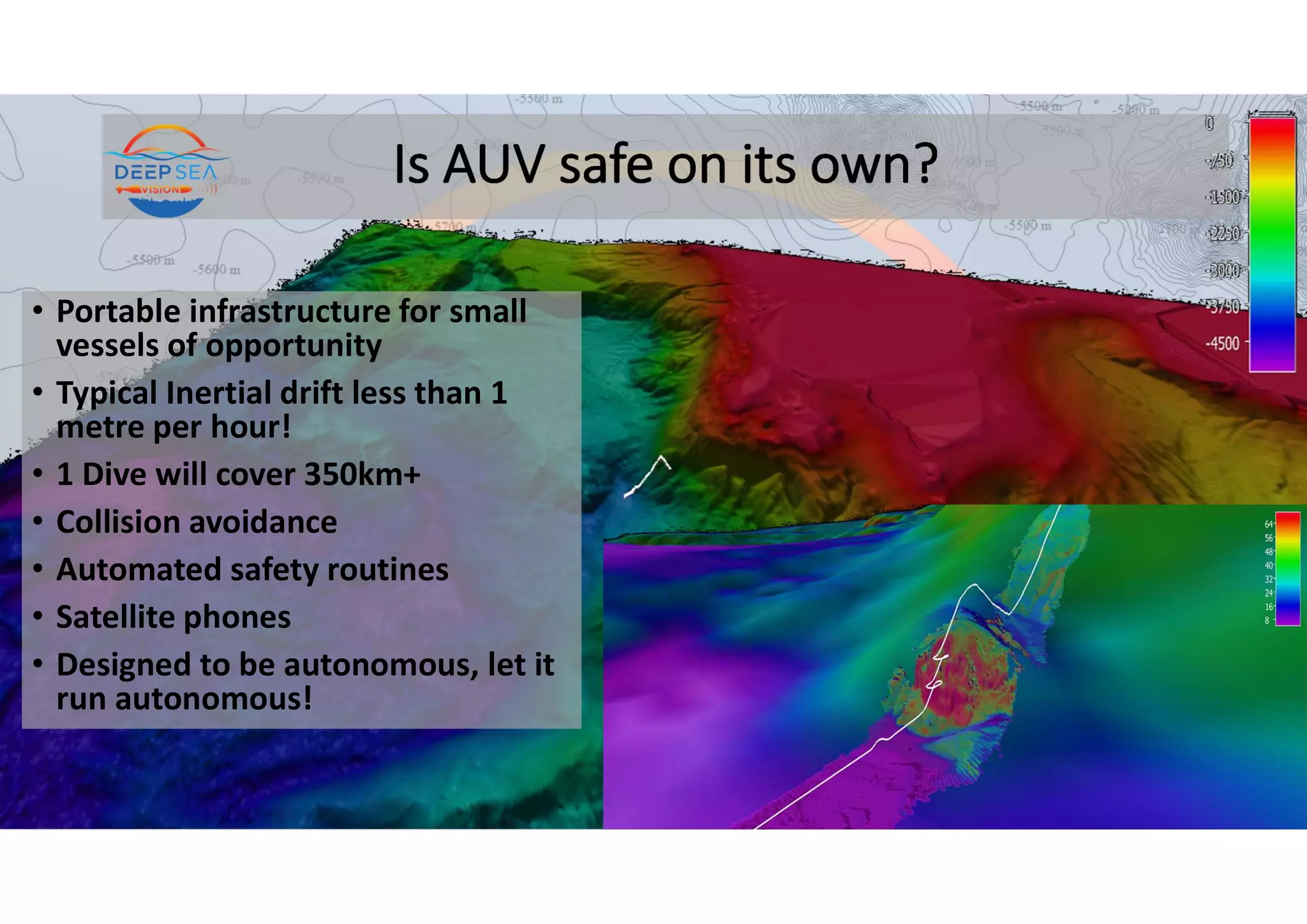
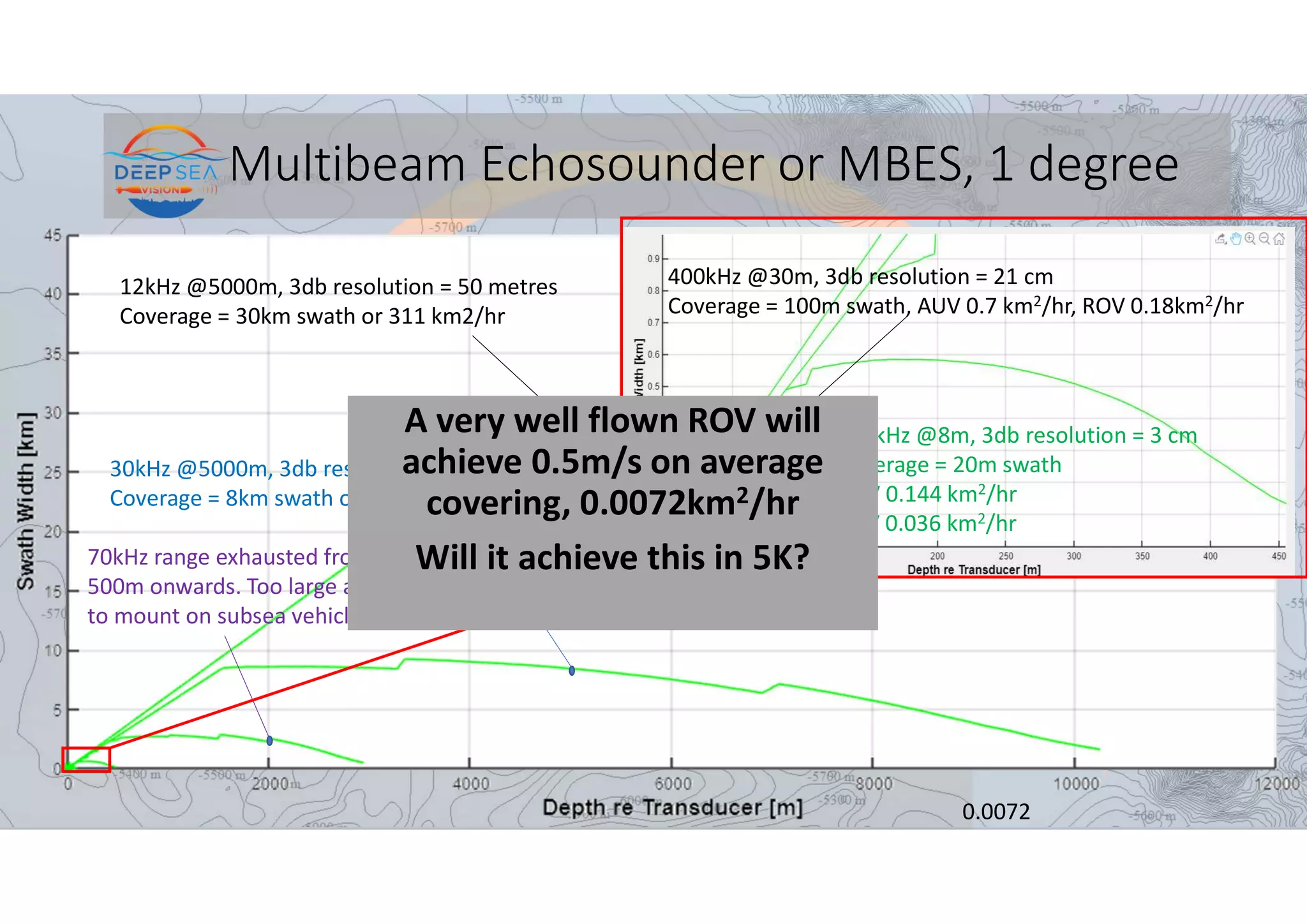
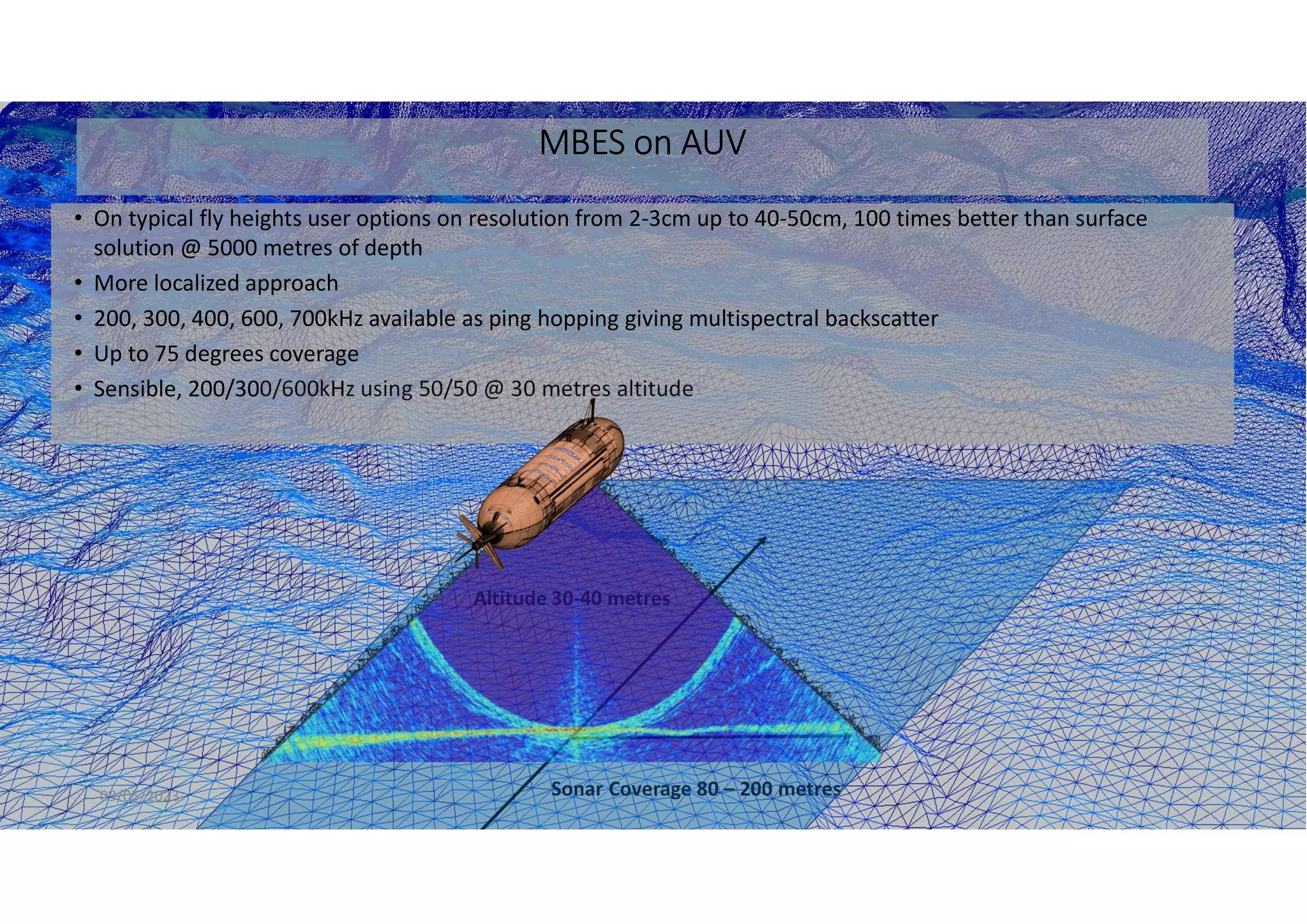
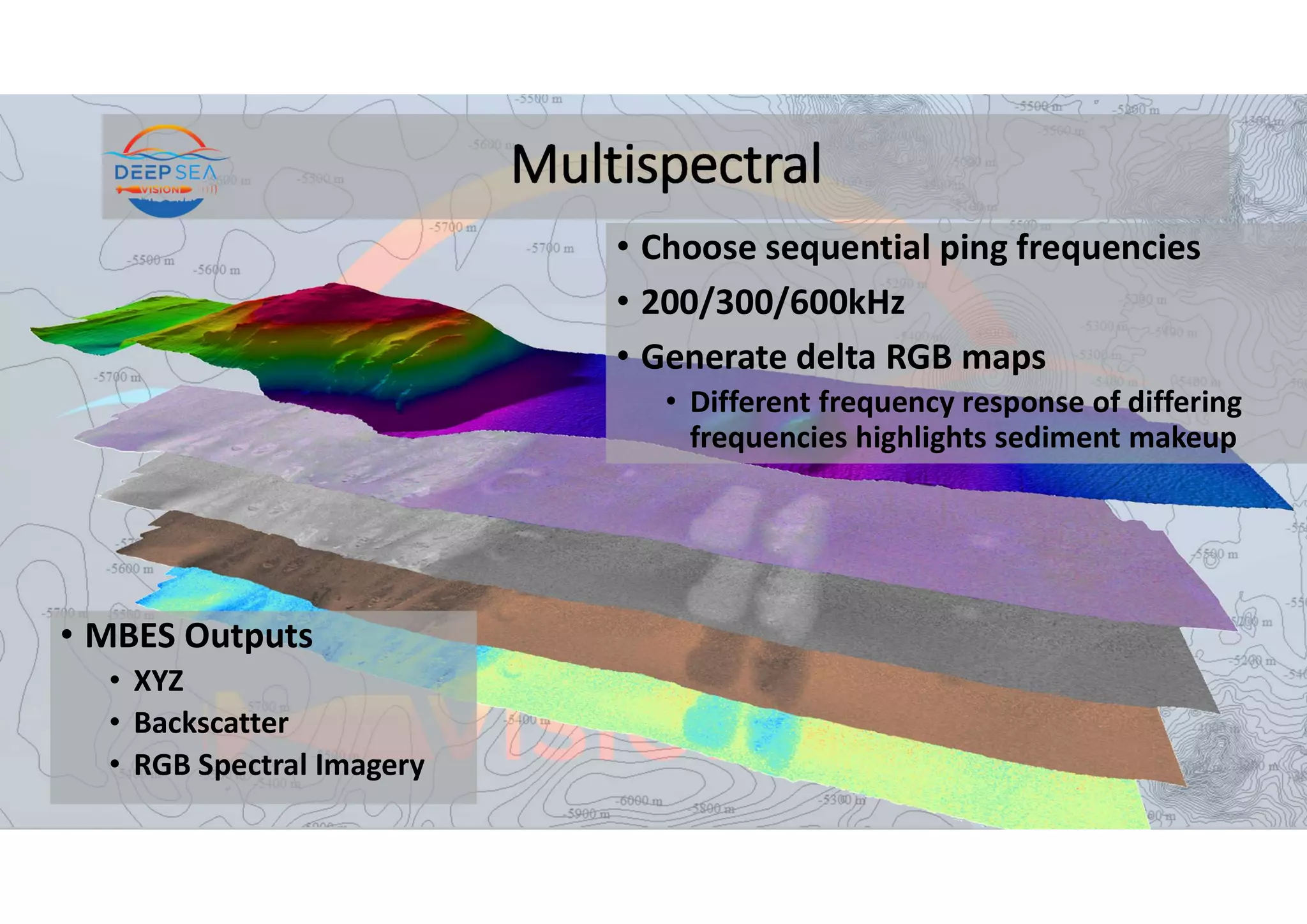
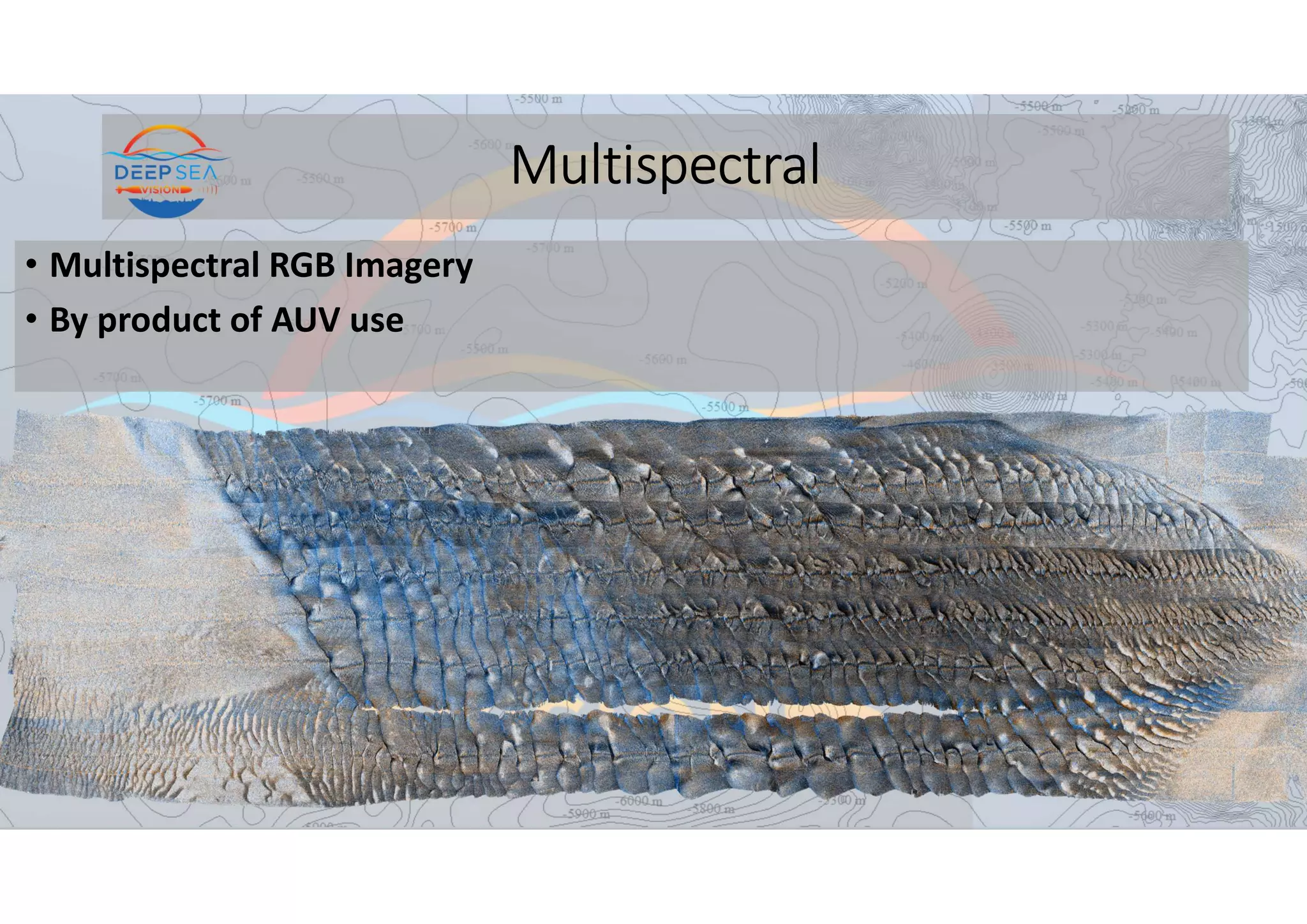
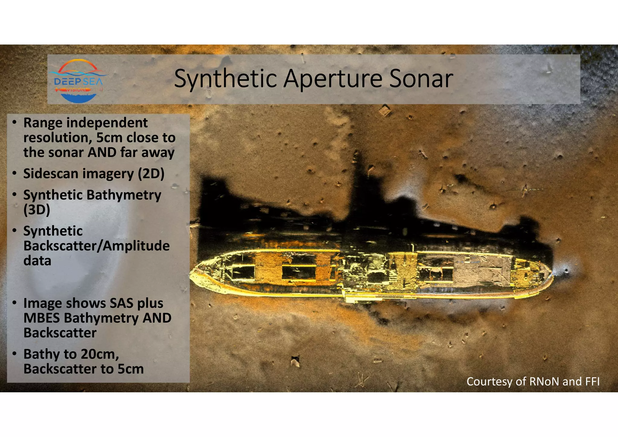
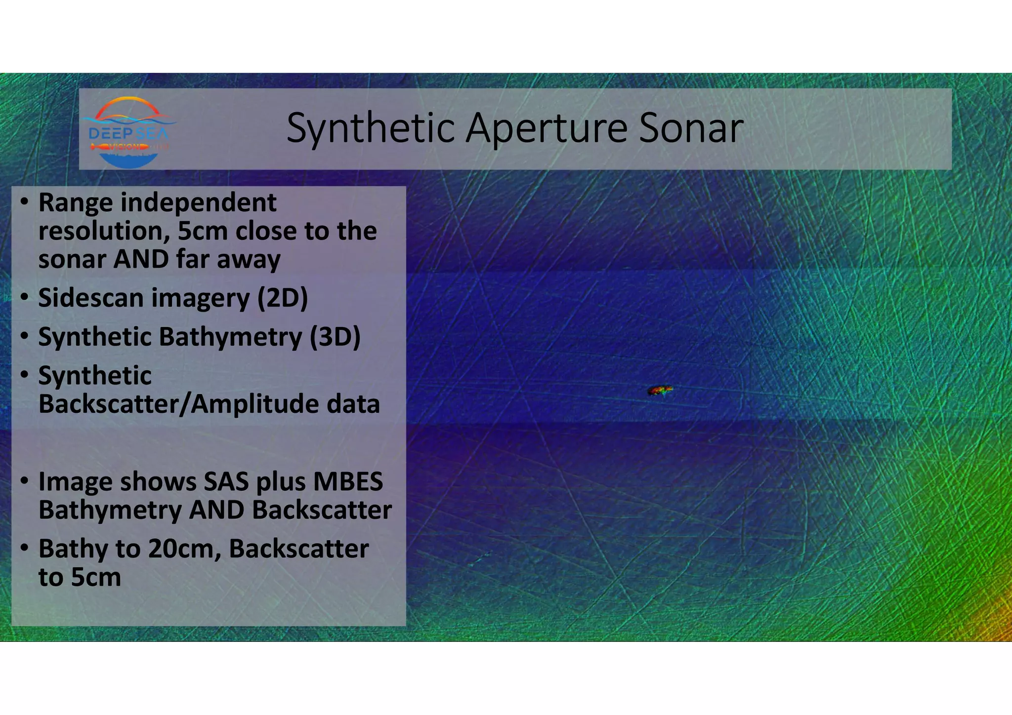
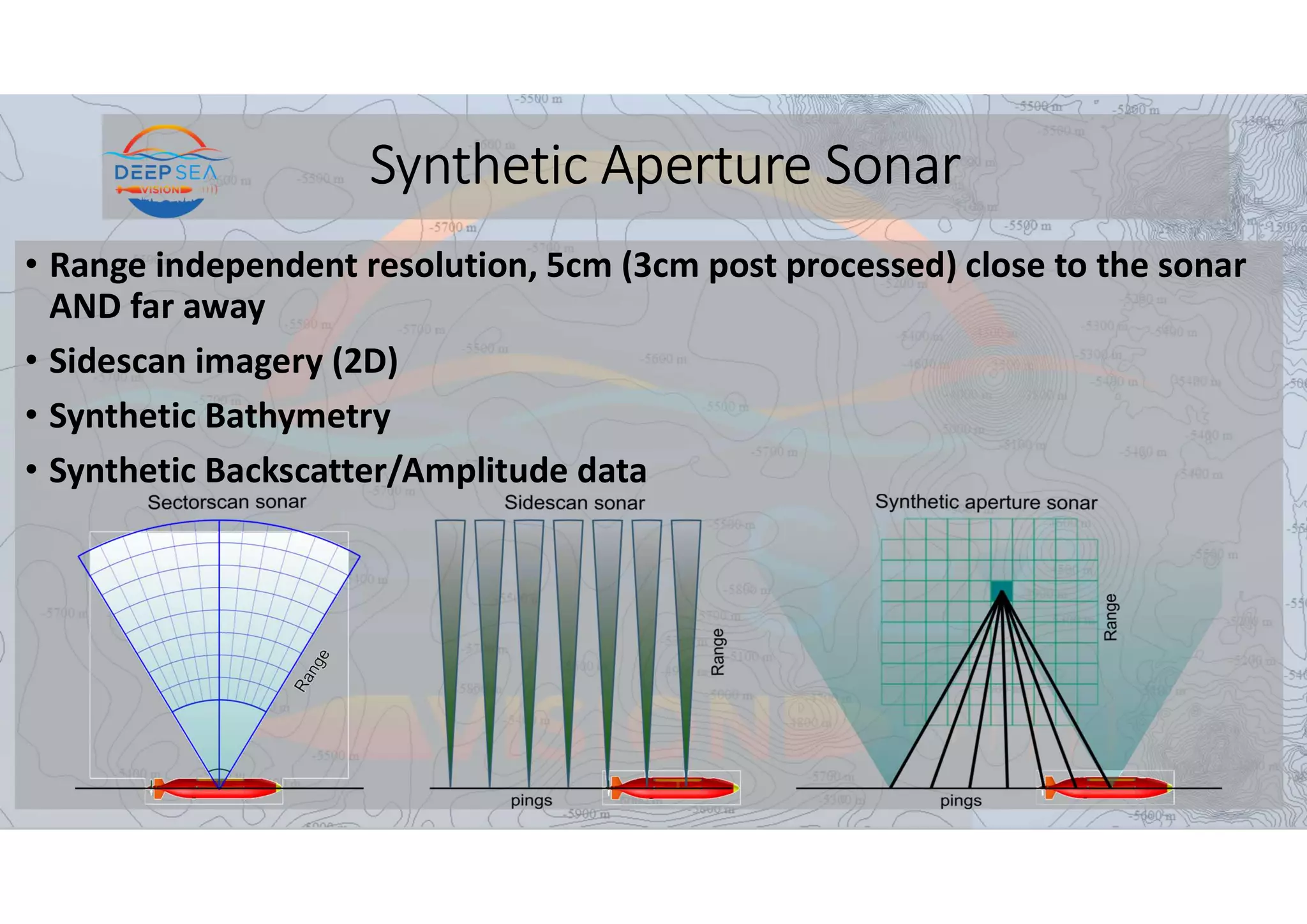
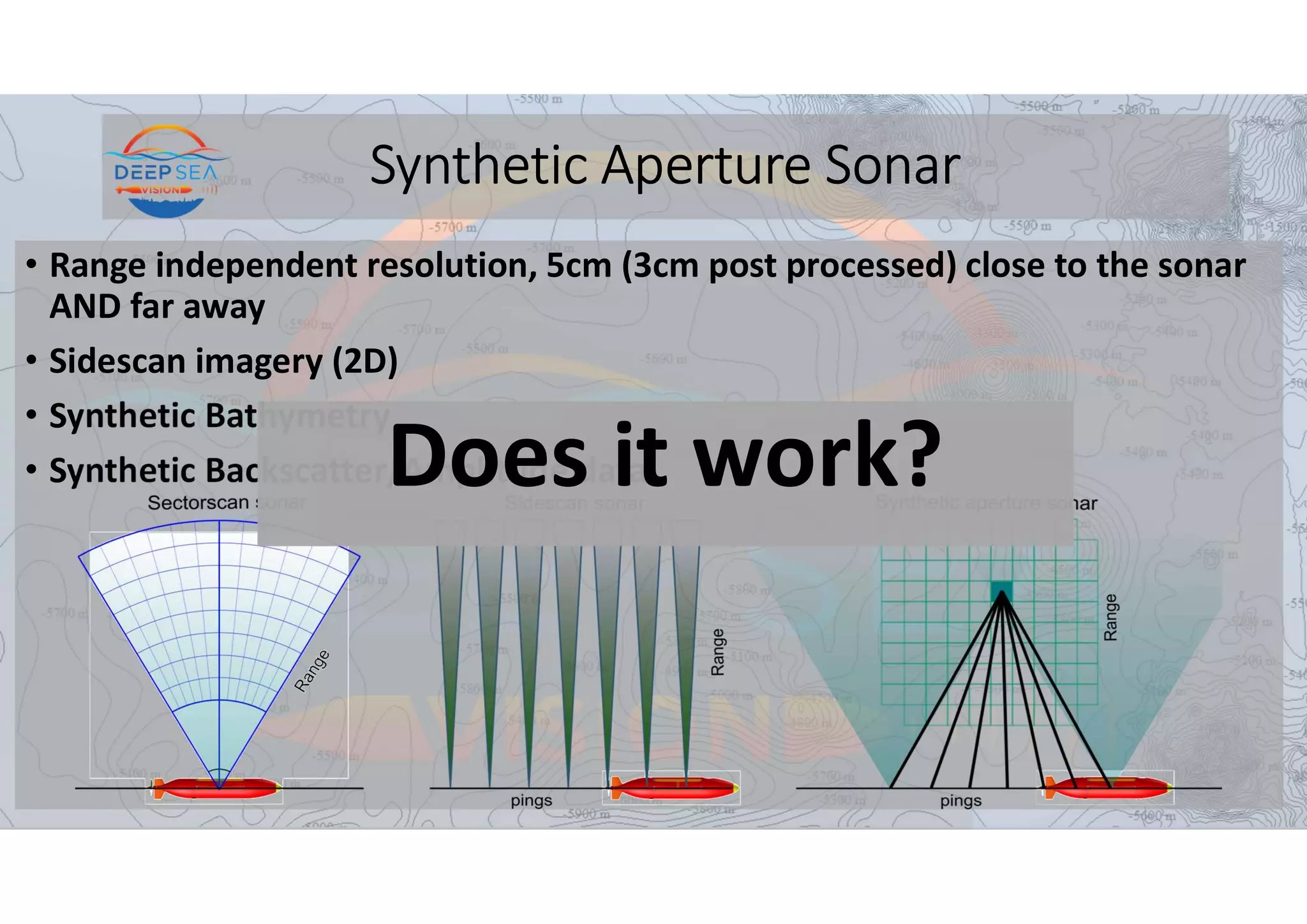
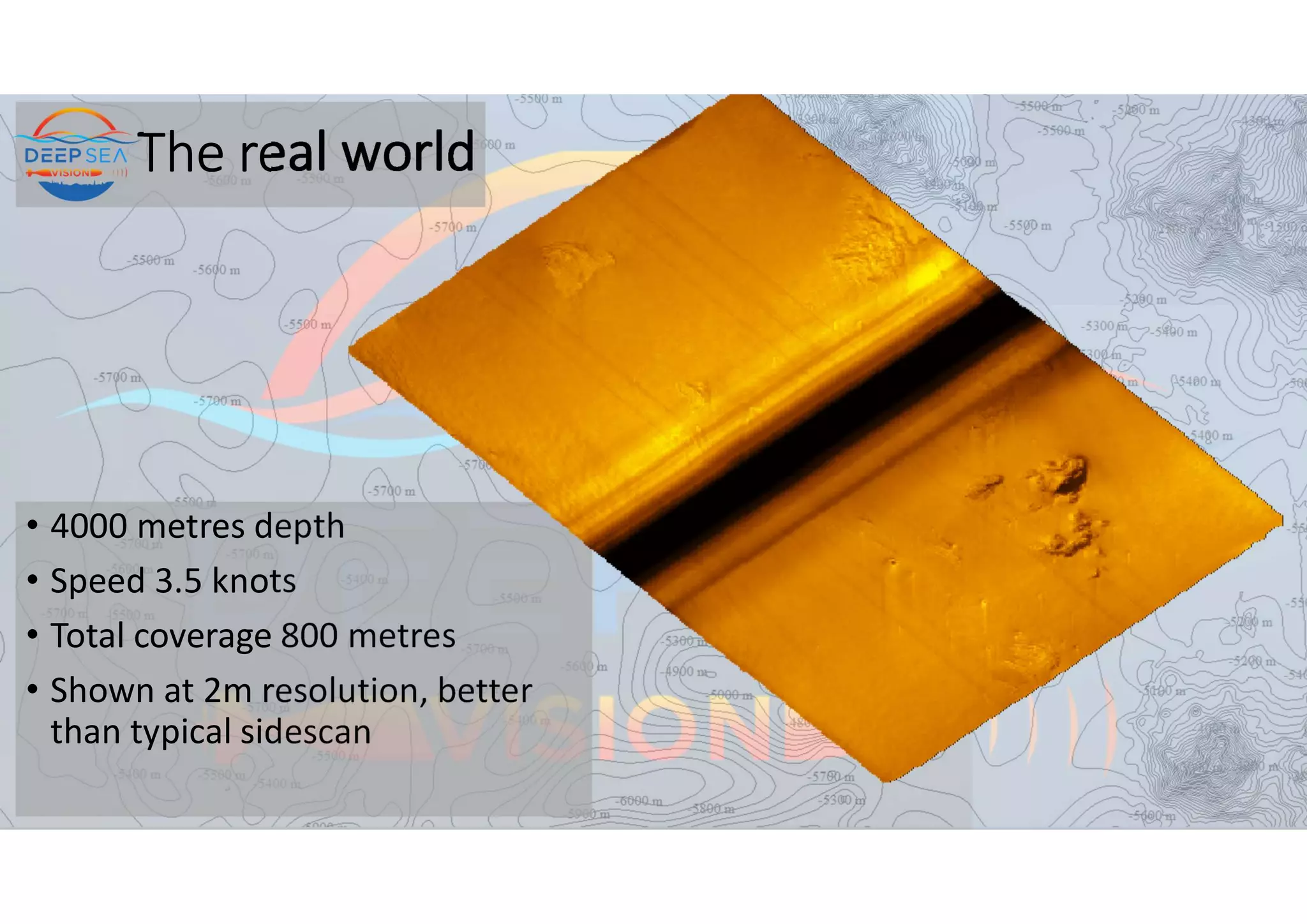
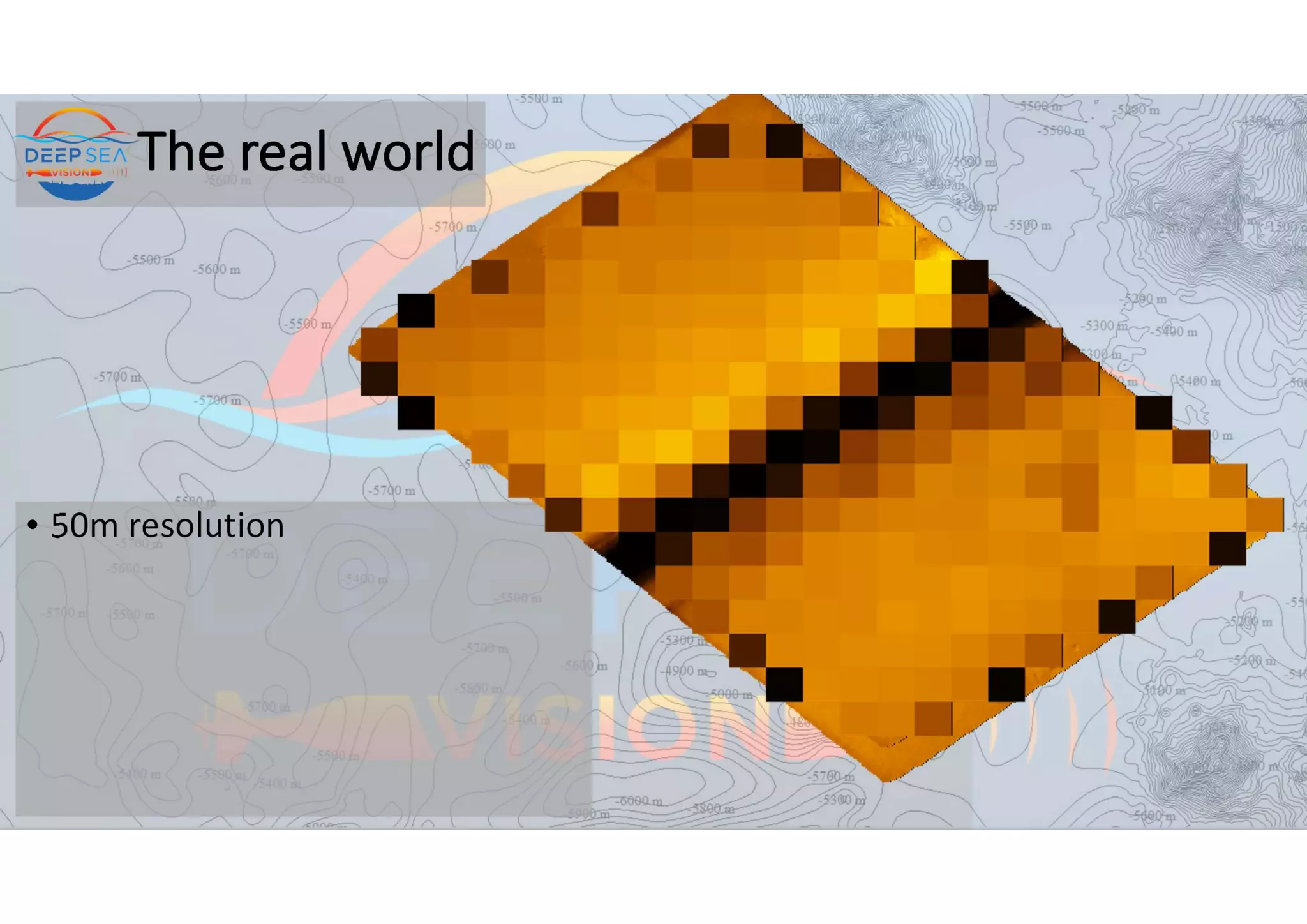
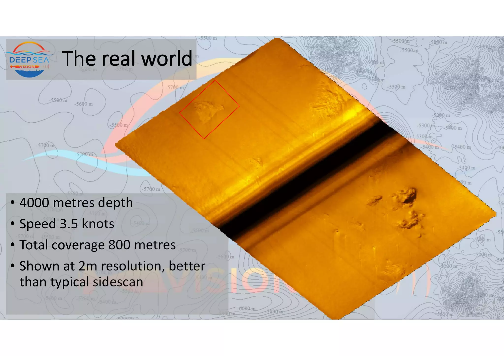
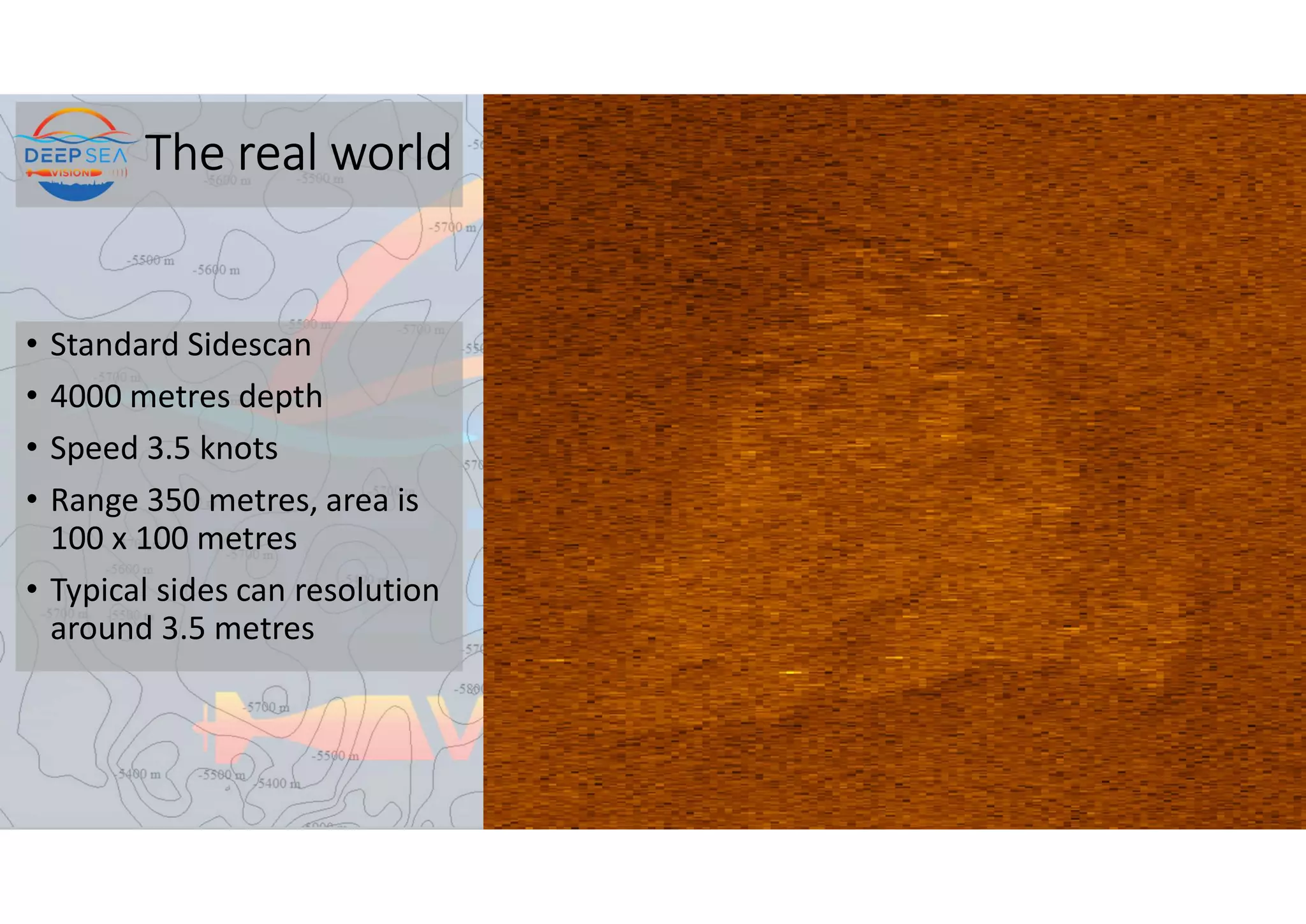
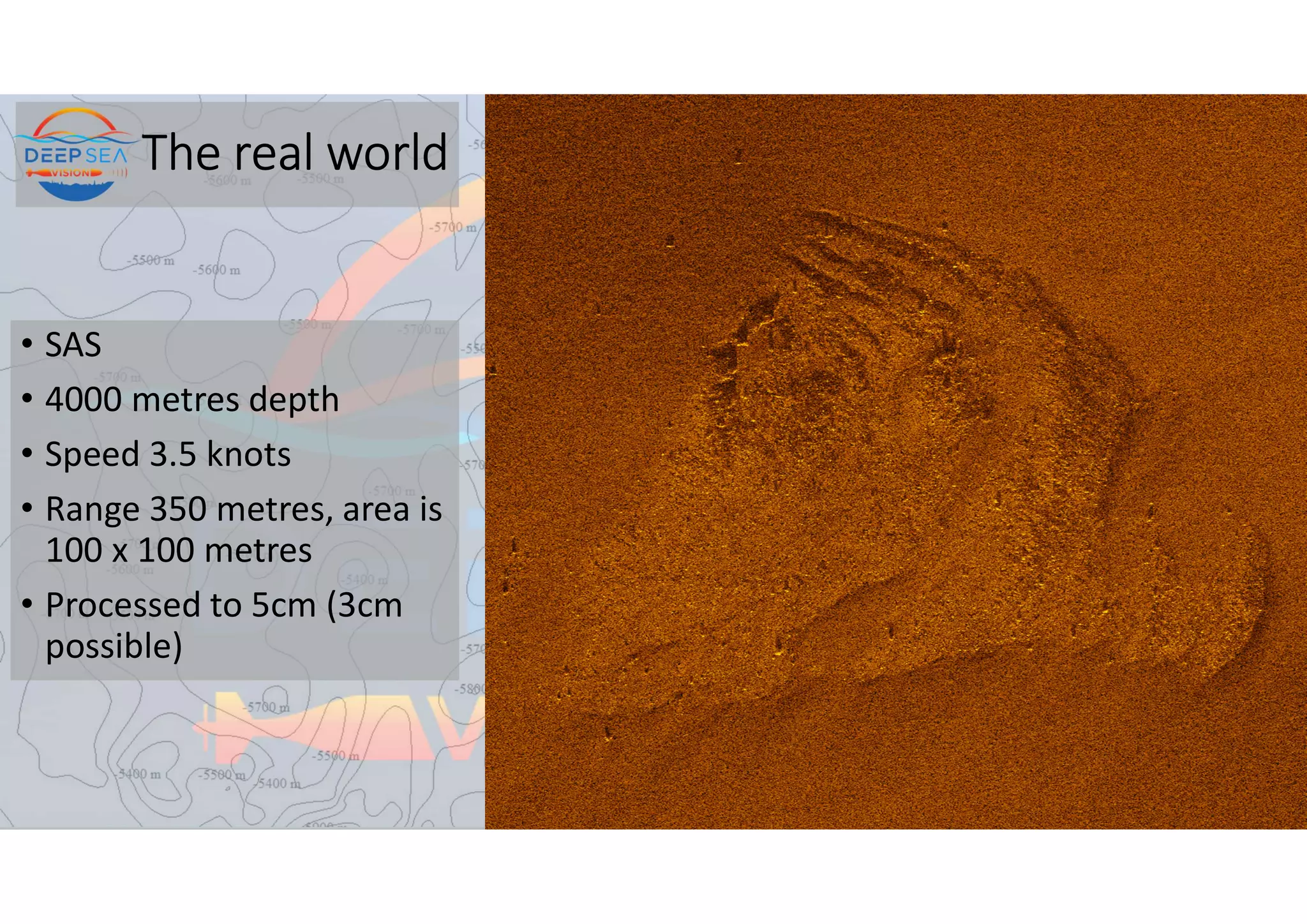
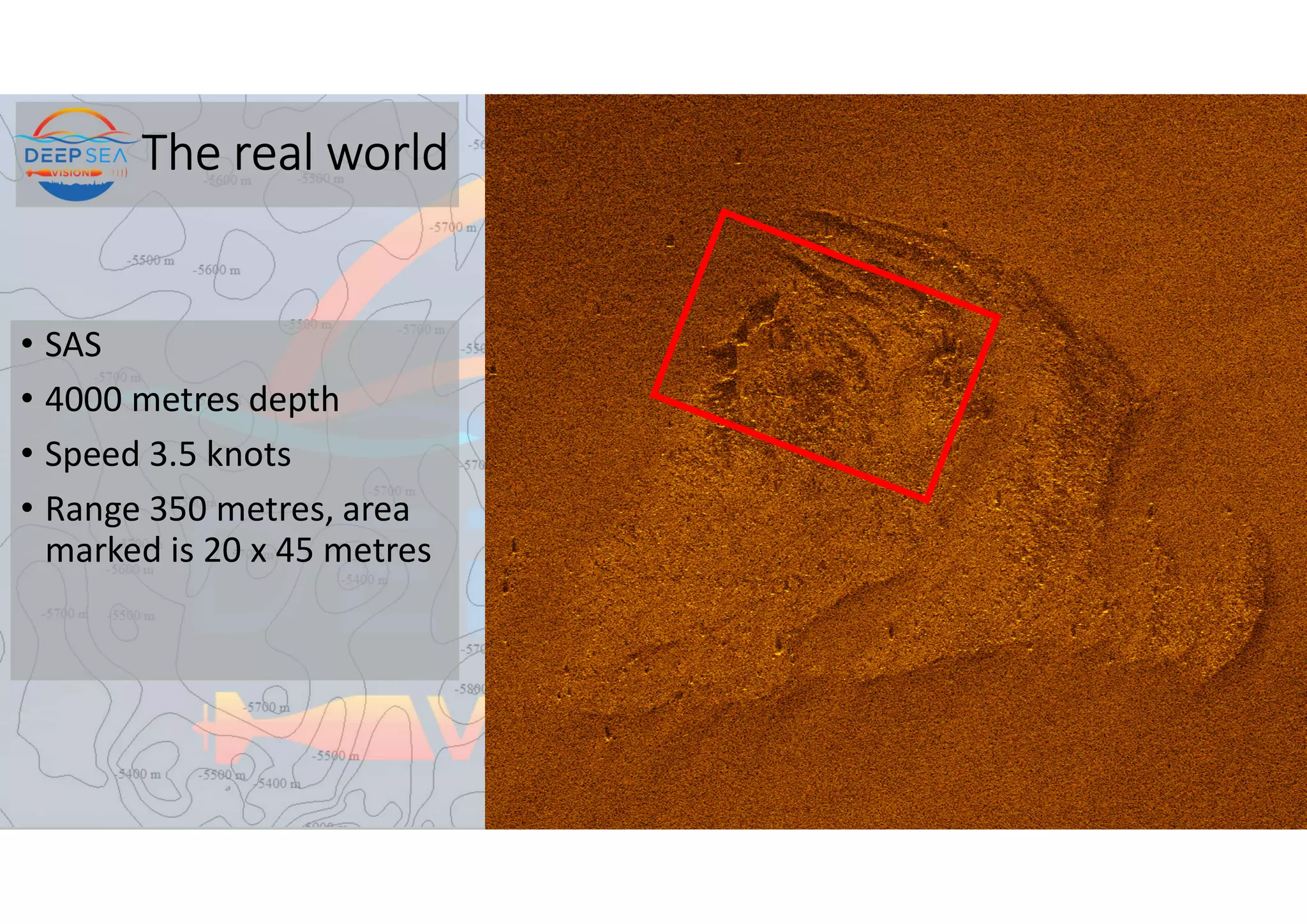
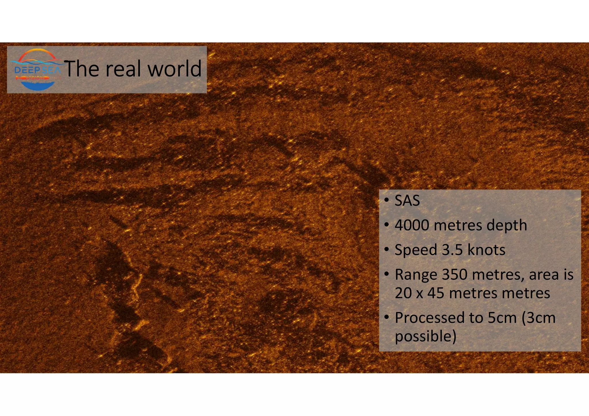
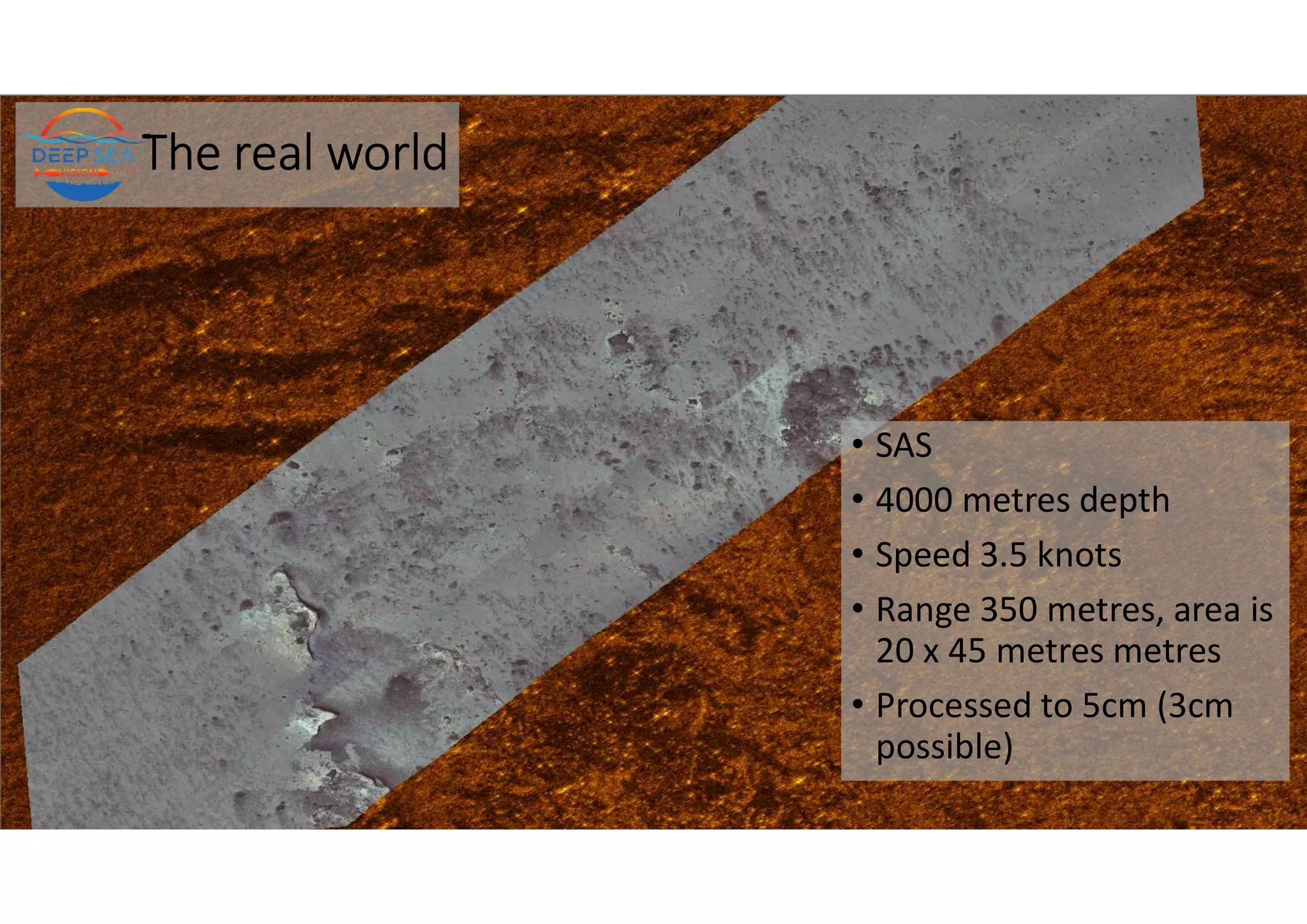
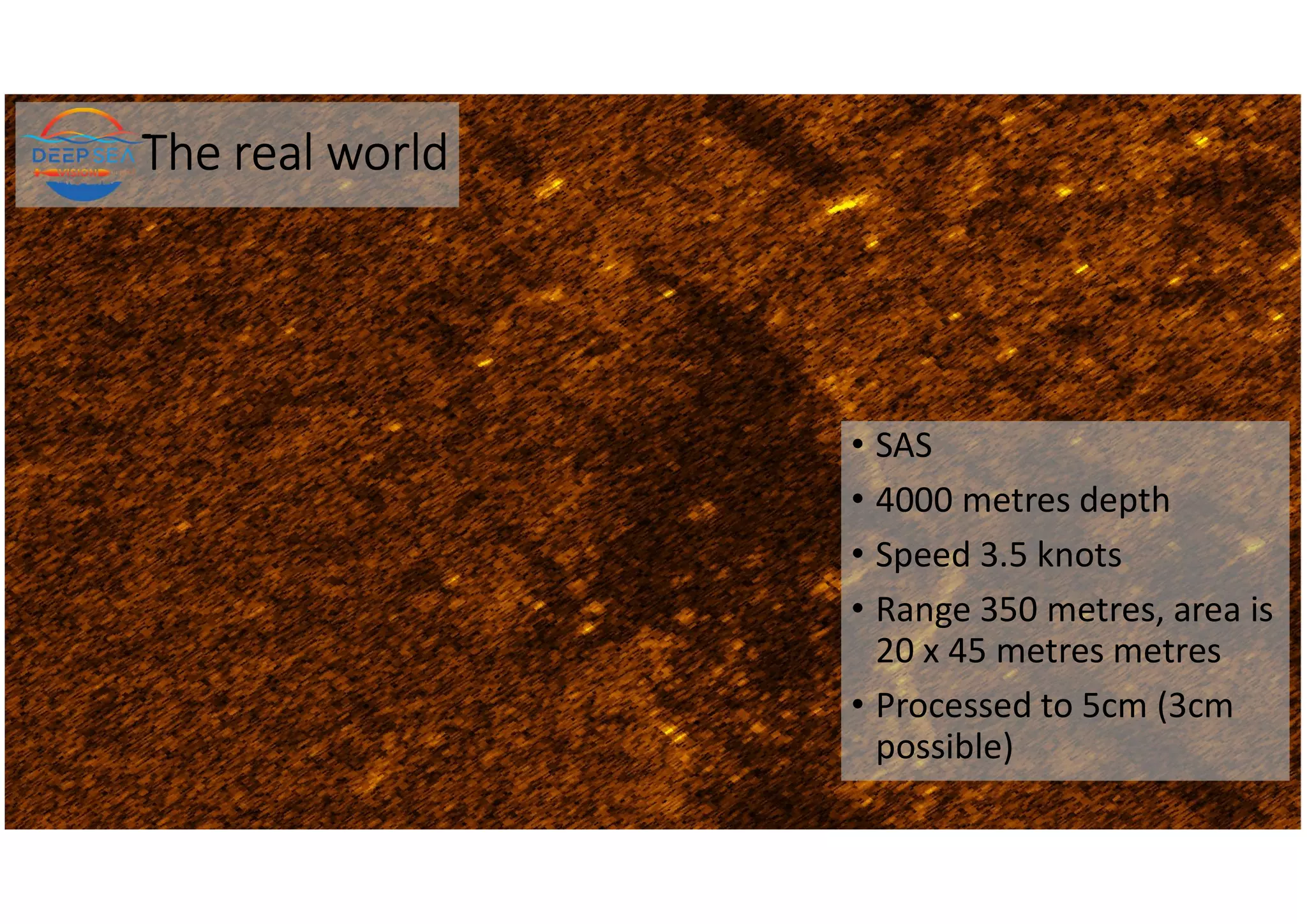
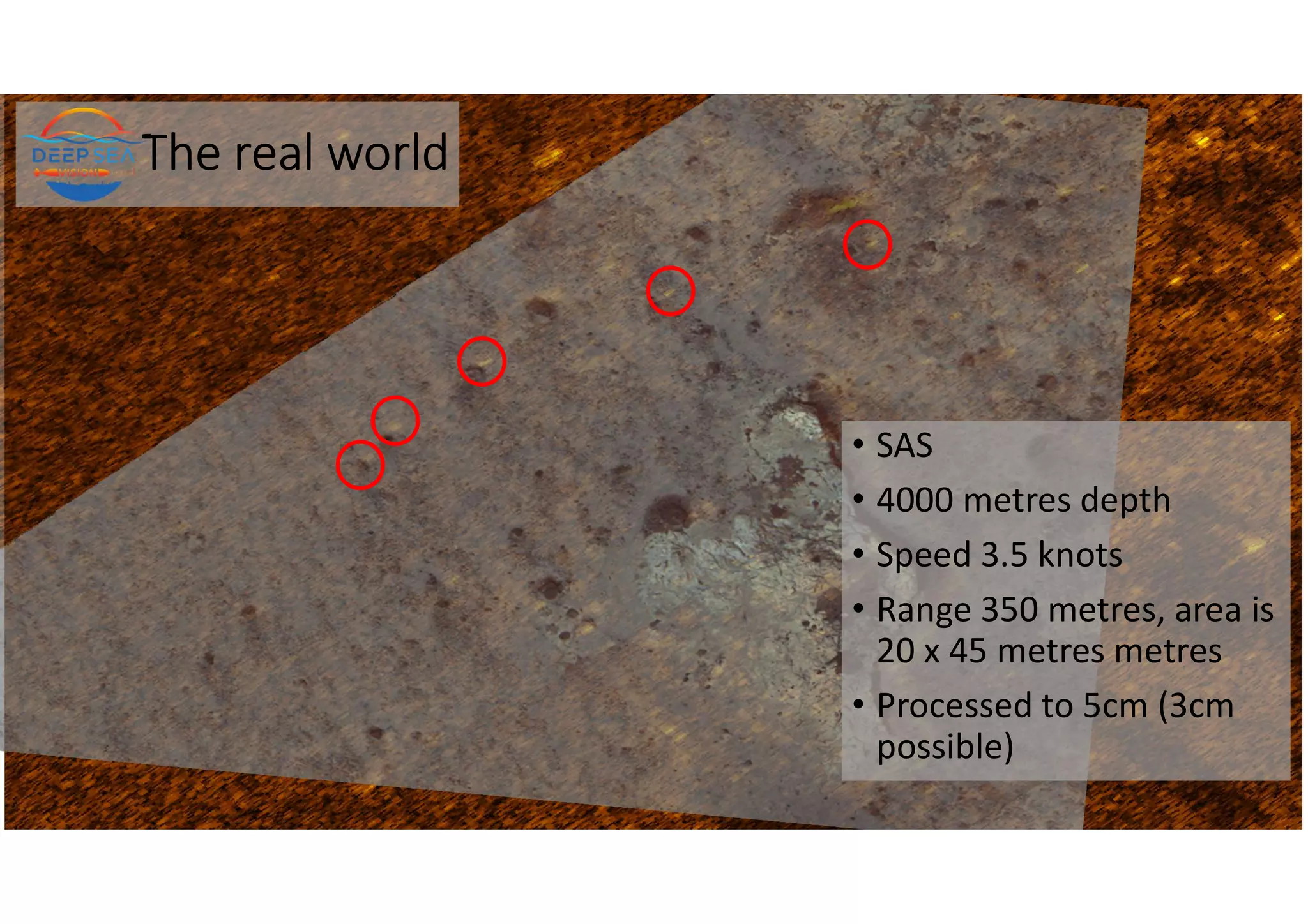
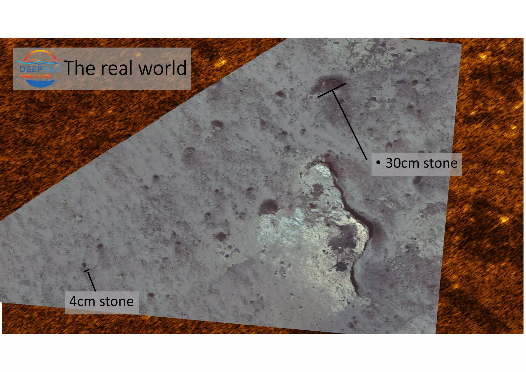
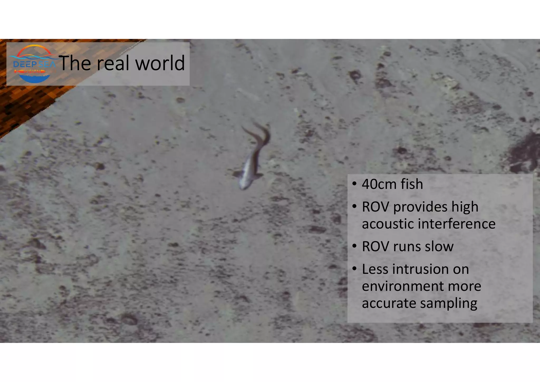
Craig Wallace
craig@deepseavision.com
An Overview of Deep Sea Surface
Mounted Mapping, ROV and AUV
Why AUV?
Agenda
• Who are DSV and who am I?
• Craig Wallace
• Deep Sea Vision
• What are the goals from a mining
perspective?
• Resolution?
• Classification?
• Coverage?
• Getting away from visual?
• Sensors
• Sub Bottom Profiler
• Camera or Video
• MBES
• Synthetic Aperture Sidescan
• Surface Mounted “MBES”
• ROV
• AUV
• Resolution versus range
• Required Infrastructure
• Cost
Craig Wallace
• Craig Wallace
• Worked for Kongsberg Maritime from
2007 through to 2022 now with Deep
Sea Vision as President of Operations
• Applications engineer?
• Government Mapping
programs,Environmental progams,
O&G, Sonar Research and Military
projects but also involed with,
• Deep Sea Tailings Pipelines
• Plume research projects
• Government Seabed Habitat and Mineral
Classification
DSV
• Company founded in 2022 from industry
experts, interests in exploration and
research, New name old experience
• HUGIN AUV Operations group
• 6000m Rated Vehicle in self contained
containers
• MBES
• Synthetic Aperture Sidescan SAS
• Camera, laser
• Magnetometers
• Environmental sensors
• Up to 100 hours endurance 50+ typical @ 3.5
knots completely unattended.
• 85%+ Duty Cycle
• Access to vessels of opportunity allowing
a turn key solution including 30kHz MBES
surface mount sonar and ROV
DSV
Our goals
• Nimble global solution but centred in the Pacific
• Turn Key Solutions,
• AUV
• Vessel
• Surface Mapping
• ROV
• Provision of cutting edge mapping technology
• Reduced operational overheads without compromise on data quality
• Complete transparency in day rates
• Realistic performance achievable, Duty Cycle Operational
• Post Processing options offering what is actually required
Mapping the Ocean Deliverables
Courtesy of RNoN and FFI
What’s needed for Mineral Mapping
• Multistage approach? Surface MBES
followed by ROV
• Target detection or mapping or both?
• 3D or 2D
• Grab samples or imagery or both
• Do we understand the forms of payload sensor above and the coverage rates
Ultimately all we want to know is material volume for
extraction, the type, transition boundaries and the impact of
extraction to the environment
Multibeam Echosounder or MBES
• Used on Surface Vessel, ROV and AUV
• Creates 3 Dimension view of seafloor
from a Mills Cross arrangement
• Outputs
• Bathymetry
• Reflectivity or Backscatter
• Extra outputs such as rugosity or
gradient maps
• Studies lead into Multispectral Data
What is the “resolution” of a MBES
• 3db Points
09/05/2023
Beam
Angle
• 0.3 – 4 degree beams typical
• Angle is a function of array length
and frequency
• Low frequency needs BIG
transducers.
• 0.5 degree 12kHz system is 16
metres long!
• 5MHz = a few decimetres range
• 400kHz perhaps 100 metres
• 12kHz gives 30km!
3db Resolution
• Complicated
• Here we see clearly the separation
of a target pair, which one are you
happy with as distinct?
• Sometimes used to describe
precision
• Question.
• Do we want mapping sonar or
an inspection sonar??
• Accurate representaion OR
shallowest point By Spencer Bliven - Own work, Public Domain,
https://commons.wikimedia.org/w/index.php?curid=31456019
Multibeam Echosounder or MBES
50cm resolution “Cell Size”
20m range 0.5 degree beams, should be 15cm?
Multibeam Echosounder or MBES
Raw data shows some targets
down to perhaps 25cm resolution
so just get closer?
And what about the 3db beam?
Multibeam Echosounder or MBES
• EM2040 High Frequency MBES @400kHz
Multibeam Echosounder or MBES
• EM2040 High Frequency MBES @600kHz
Multibeam Echosounder or MBES
• EM2040 High Frequency MBES @700kHz
LOCH NESS MONSTER BACKSCATTER
Perhaps a 50%
improvement in mosaic
resolution due to
sampling resolution
Note that traditionally
target size must be 5 - 10
times greater than
wavelength
300kHz > 5mm
30kHz > 50mm
12khz > 15cm
LOCH NESS MONSTER BACKSCATTER
Perhaps a 50%
improvement in mosaic
resolution due to
sampling resolution
Note that traditionally
target size must be 5 - 10
times greater than
wavelength
300kHz > 5mm
30kHz > 50mm
12khz > 15cm
• All at close range with high frequency portable
MBES
• How do the deep water systems compare?
12kHz @5000m, 3db resolution = 50 metres
Coverage = 30km swath or 311 km2/hr
Hull mounted Multibeam Echosounder or
MBES, 1 degree
30kHz @5000m, 3db resolution = 50 metres
Coverage = 8km swath or 86 km2/hr
70kHz range exhausted from around
500m onwards. Too large a system
to mount on subsea vehicle
12kHz @5000m, 3db resolution = 50 metres
Coverage = 28 – 30 km swath or 311 km2/hr
Line spacing in 5000 metres
30kHz @5000m, 3db resolution = 50 metres
Coverage = 8km swath or 86 km2/hr
70kHz range exhausted from around
500m onwards. Too large a system
to mount on subsea vehicle
• Using 100% overlap
• 12kHz system (EM124) perhaps 12km lines
• 50m “resolution”
• 30kHz system (EM304) perhaps 3km lines
• 50m “resolution”
• For comparison
• HUGIN AUV with Synthetic Aperture sonar
• 1000m swath but 600m realistic
comparison
• 5cm “resolution” on “targets”
Coverage Deep Water MBES
• https://ars.els-cdn.com/content/image/1-s2.0-S0967063720300698-gr5_lrg.jpg
Coverage Deep Water MBES
• https://ars.els-cdn.com/content/image/1-s2.0-S0967063720300698-gr5_lrg.jpg
SURFACE MOUNT DEEP WATER BACKSCATTER
• Typical C1 – C5 geological classification
- So what more do you need?
- ROV grab samples and we are done?
Description
Seabed geological class
Most sta ons are clay sediment. Average backsca er intensity is −42.1 dB ranging from -38
to -47dB. Average abundance is 4.8 kg/m2. 4150 km2
C1-Pelagic clay sediment, basin
Average backsca er intensity is −38 dB.
C2-Calcareous pelagic sediment, seamount
Average backsca er intensity is −32.9 dB. Average nodule abundance is 19.8 kg/m2.
14900km2
C3-Nodules with abundance around
20 kg/m2, basin
Average backsca er intensity is −29.1 dB. Average abundance is 39.6 kg/m2. Note central
area which “Might” have the largest abundance of 6cm nodules
C4-Nodules with abundance around
40 kg/m2, basin
Average backsca er intensity is −22.5 dB
C5-Cobalt-rich crust, seamount
SURFACE MOUNT DEEP WATER BACKSCATTER
• 5dB on this map can be up to 30 or 40km! @ 20Kg per cubic metre
- Surface Impedance is a function of many factors which results in an unacceptable variation in backscatter transition zones
- Multi spectral high frequency MBES would provide more insight
- Transition zones of backscatter maps when cross reference to gradient maps can be a useful first assessment for mineral
deposits if collection costs are low
• Is grab samples
enough?
• A single sample
in 5km could
take 9 hours or
more
• Transition
zones have
high
uncertainty
SURFACE MOUNT DEEP WATER BACKSCATTER
• We see 3.9dB variation between C3 and C4, the difference is 19.8 kg/m2 or 40kg/m2
• 3rd Party processing software shows a 10dB variation between them
• A “calibrated” sonar can show 5-10 dB variation
• What if not even normalised? That’s 5db between sectors and 3db between passes
The problem
• Surface MBES can give good
indications
• Huge focus on the verification of
material presence
• Delineation of transitions is what
actually matters
Transects of Hi resolution data are
required; spot samples require high
density (better than every 40km)
• Goodness fit up to 80%
• https://www.researchgate.net/publication/340316836_Acoustic_quantitative_analysis_of_ferromanganese_nodule_and_
cobalt-rich_crust_distribution_areas_using_EM122_multibeam_backscatter_data_from_deep-
sea_basin_to_seamount_in_Western_Pacific_Ocean
• “The shipboard MBES data, in combination with continuous video footage of the seabed, exhibited a positive
correlation between high backscatter intensity, steep seabed slopes, and the occurrence of Fe–Mn crusts, but
these observations were insufficient to discriminate the spatial boundaries between several seabed types that
occurred” 12KHz MBES in 2000-3000m of depth
• https://www.mdpi.com/2075-163X/10/2/155
Marine Salvage
“A science of vague assumptions based
on debatable figures taken from
inconclusive experiments and
performed with instruments of
problematic accuracy by persons of
doubtful reality and questionable
mentality.”
Capt C.A “ Black Bart” Bartholomew
https://usnamemorialhall.org/images/7/72/196
1_Bartholomew_LB.jpg
SURFACE MOUNT DEEP WATER BACKSCATTER
• Do we need to map the whole area
100%?
• Is 40km too large a loss? Where is
the balance acceptable
• Deep water MBES does provide a
benefit but could it be removed?
• Quadrat estimations have been
used without issue for lots of
ecosystems to date
AUV
A sparse but very high resolution
grid with extra data provides a more
efficient overall solution
SURFACE MOUNT DEEP WATER BACKSCATTER
• Grid survey is required with spacing based on deep water backscatter interpretation
• ROV/AUV and which sensor?
ROV
ROV and AUV
Pros
• Can be alive 24 hours/day
• Grab samples
• Real time interaction
Cons
• Expensive running costs
• Slow speed, 0.5 up to 1 knot average (Unlikely in
5Km) low coverage rate
• Constant mothership support
• Limited weather window
• Video standard only
• INS/Decent Payload all add to cost
• Platform instability too poor for high end sensors
• Long ascent and descent times (5K typical 2.5 hours)
AUV
Pros
• Achieve 85 -90% Duty Cycle
• Lower operational cost
• Typical 3 - 4 knot survey speed (4 times faster min)
• Wide weather window
• Lesser Observer effect on marine life
• Low human risk factor, controlled collection
• Large selection of sensors integrated by design
• Allows mothership activities out with AUV ops
• Better data quality WRT sonar
• Reasonable ascent and descent, (5K typical 1 hour)
Cons
• No grab samples
Proposed AUV grid solution
Fully Autonomous with no Mothership
acoustic tethering, all automated
planning
• Run concurrent at 30-40m alt
• SBP (not favored at ROV or camera
altitude)
• MBES including multi-spectral
• HISAS Synthetic Aperture Sonar
• Intersections looped at 5m alt
• Camera / Laser
• Magnetometer
• Always logging Environmental sensors
1st Pass, HISAS 400 – 1000m
1st Pass, Multispectral 100m
1st Pass, SBP transect
2nd Pass, Camera
2nd Pass, Maggy
2nd Pass, Enviro
Proposed AUV grid solution
Fully Autonomous with no
Mothership acoustic tethering, all
automated planning
• Grid spacing becomes a function of
operator resources
• More efficient methods to ensure
less waste
1st Pass, HISAS 400 – 1000m
1st Pass, Multispectral 100m
1st Pass, SBP transect
2nd Pass, Camera
2nd Pass, Maggy
2nd Pass, Enviro
EM304 Hypothetical 300km x 300km area, 5k
Nominal depth
• EM304 vessel, estimated coverage 8km,
line spacing 4km.
• 75 lines @ 28 hours per line plus 25% for
turns and standard weather = 95 days
• Vessel cost ~25K USD/Day 2.4M USD
• Processing (Inc Backscatter) perhaps
$4K/USD day and allow 2:1 = 350K USD
• 3m USD before calibration etc etc.
• 153 days, 100% ensonfication at low resolution 0.0001% high
resolution
• 5M USD plus
• Full ROV coverage clearly not an option
• Resultant 100% coverage to very low resolution, 50 metres,
backscatter to perhaps 20.
• Extremely limited high-resolution data
Good enough?
• ROV vessel, $35K USD/Day
• Grab Samples, perhaps 8 hours per
sample on perhaps 20km spacing is
100 samples and 2500 line km = 25
days in transits, 33 in samples total
58 days
• 2.0M USD before personnel etc etc.
EM 124 Hypothetical 300km x 300km area,
5k Nominal depth
• EM122, estimated coverage 25km, line spacing
15km.
• 24 lines @ 28 hours per line plus 25% for turns
and standard weather = 35 days
• Vessel cost ~35K USD/Day 1.25M USD
• Processing (Inc Backscatter) perhaps $4K/USD
day and allow 2:1 = 280K USD
• 1.5m USD before calibration, personnel etc etc.
• 100 days, 100% ensonfication at low resolution 0.0001% high
resolution
• 3.5M USD excluding transits
• Vessel needed for 80 days+
• Resultant 100% coverage to very low resolution, 50 metres,
backscatter to perhaps 20m.
• Extremely limited high-resolution data
Good enough?
• ROV vessel, $35K USD/Day
• Grab Samples, perhaps 8 hours per
sample on perhaps 20km spacing is
100 samples and 2500 line km = 25
days in transits, 33 in samples total
58 days
• 2.0M USD before personnel etc.
Hypothetical 300km x 300km area, 5k
Nominal depth
• AUV vessel solution using synthetic aperture sonar ~ 30K USD/Day and could
accommodate concurrent ROV sampling, an extra 15K USD/Day
• 600m corridors (5cm resolution) spaced 15km apart gives 20 lines, 46 hours per line
plus additional 10% for inspection inclusion is 50 hours per line or 42 days for complete
grid
• Allow for 85% duty cycle gives 48 days = $1.5 M USD for complete grid
• Vessel is free for concurrent ROV grab sampling, is 1.5 M USD OR EM304/EM124 work
• 1.5 M USD excluding transits and fuel but notably halved as one vessel
• Less fuel
• Less Personnel
• Less transits
• Less Risk
• Magnitudes more conclusive than previous solution with 5cm resolution over the
complete grid including all other payload sensors
• Grid spacing becomes a function of resources
Is AUV safe on its own?
• Portable infrastructure for small
vessels of opportunity
• Typical Inertial drift less than 1
metre per hour!
• 1 Dive will cover 350km+
• Collision avoidance
• Automated safety routines
• Satellite phones
• Designed to be autonomous, let it
run autonomous!
Camera, Video or Stills
• Video was the industry standard, better for slow
moving vehicles
• 4 metre corridor
• High backscattering, constant high power light
source.
• Good for humans, bad for marine life
• Human interpretable data
• Stills are georeferenced with mission data
• Simple mosaicking
• Higher resolution
• Quantifiable data
• Lesser Observer Effect
18cm
SBP
• 2 – 16kHz standard
• Up to 60m penetration ~10cm
resolution
• Option on
• 1-6kHz 100m penetration ~15cm
• 4-24kHz 40m ~7.5cm
12kHz @5000m, 3db resolution = 50 metres
Coverage = 30km swath or 311 km2/hr
AUV sonar?
30kHz @5000m, 3db resolution = 50 metres
Coverage = 8km swath or 86 km2/hr
70kHz range exhausted from around
500m onwards. Too large a system
to mount on subsea vehicle
12kHz @5000m, 3db resolution = 50 metres
Coverage = 30km swath or 311 km2/hr
Multibeam Echosounder or MBES, 1 degree
30kHz @5000m, 3db resolution = 50 metres
Coverage = 8km swath or 86 km2/hr
70kHz range exhausted from around
500m onwards. Too large a system
to mount on subsea vehicle
400kHz @30m, 3db resolution = 21 cm
Coverage = 100m swath, AUV 0.7 km2/hr, ROV 0.18km2/hr
600kHz @8m, 3db resolution = 3 cm
Coverage = 20m swath
AUV 0.144 km2/hr
ROV 0.036 km2/hr
0.0072
A very well flown ROV will
achieve 0.5m/s on average
covering, 0.0072km2/hr
Will it achieve this in 5K?
09/05/2023
• On typical fly heights user options on resolution from 2-3cm up to 40-50cm, 100 times better than surface
solution @ 5000 metres of depth
• More localized approach
• 200, 300, 400, 600, 700kHz available as ping hopping giving multispectral backscatter
• Up to 75 degrees coverage
• Sensible, 200/300/600kHz using 50/50 @ 30 metres altitude
Altitude 30-40 metres
MBES on AUV
Sonar Coverage 80 – 200 metres
Multispectral
• MBES Outputs
• XYZ
• Backscatter
• RGB Spectral Imagery
• Choose sequential ping frequencies
• 200/300/600kHz
• Generate delta RGB maps
• Different frequency response of differing
frequencies highlights sediment makeup
Multispectral
• Multispectral RGB Imagery
• By product of AUV use
Synthetic Aperture Sonar
• Range independent
resolution, 5cm close to
the sonar AND far away
• Sidescan imagery (2D)
• Synthetic Bathymetry
(3D)
• Synthetic
Backscatter/Amplitude
data
• Image shows SAS plus
MBES Bathymetry AND
Backscatter
• Bathy to 20cm,
Backscatter to 5cm
Courtesy of RNoN and FFI
Synthetic Aperture Sonar
• Range independent
resolution, 5cm close to the
sonar AND far away
• Sidescan imagery (2D)
• Synthetic Bathymetry (3D)
• Synthetic
Backscatter/Amplitude data
• Image shows SAS plus MBES
Bathymetry AND Backscatter
• Bathy to 20cm, Backscatter
to 5cm
Synthetic Aperture Sonar
• Range independent resolution, 5cm (3cm post processed) close to the sonar
AND far away
• Sidescan imagery (2D)
• Synthetic Bathymetry
• Synthetic Backscatter/Amplitude data
Synthetic Aperture Sonar
• Range independent resolution, 5cm (3cm post processed) close to the sonar
AND far away
• Sidescan imagery (2D)
• Synthetic Bathymetry
• Synthetic Backscatter/Amplitude data
Does it work?
“Target Garden”
• Targets left to right are
5cm, 7.5cm and 12cm
respectively
• Filled with concrete
“Target Garden”
• Targets left to right are
5cm, 7.5cm and 12cm
respectively
• Filled with concrete
• Range of 120 metres
• 20mm rope clearly
shown and targets
visible
“Target Garden”
• Range of 300 metres
• Defined 12.5cm targets, clear
7.5cm with 5cm still visible
• The cube also noted and the
strong reflecting corner eyelets
/ 52 / 9-May-23
HISAS Bathymetry
- Incredibly beautiful with wide swath
- Near seamless overlap with EM2040
- Giving around 25cm worst case
resolution across a 750 metre wide
swath all including co-registered
Imagery and backscatter
The real world
• 4000 metres depth
• Speed 3.5 knots
• Total coverage 800 metres
• Shown at 2m resolution, better
than typical sidescan
The real world
• 50m resolution
The real world
• 4000 metres depth
• Speed 3.5 knots
• Total coverage 800 metres
• Shown at 2m resolution, better
than typical sidescan
The real world
• Standard Sidescan
• 4000 metres depth
• Speed 3.5 knots
• Range 350 metres, area is
100 x 100 metres
• Typical sides can resolution
around 3.5 metres
The real world
• SAS
• 4000 metres depth
• Speed 3.5 knots
• Range 350 metres, area is
100 x 100 metres
• Processed to 5cm (3cm
possible)
The real world
• SAS
• 4000 metres depth
• Speed 3.5 knots
• Range 350 metres, area
marked is 20 x 45 metres
The real world
• SAS
• 4000 metres depth
• Speed 3.5 knots
• Range 350 metres, area is
20 x 45 metres metres
• Processed to 5cm (3cm
possible)
The real world
• SAS
• 4000 metres depth
• Speed 3.5 knots
• Range 350 metres, area is
20 x 45 metres metres
• Processed to 5cm (3cm
possible)
The real world
• SAS
• 4000 metres depth
• Speed 3.5 knots
• Range 350 metres, area is
20 x 45 metres metres
• Processed to 5cm (3cm
possible)
The real world
• SAS
• 4000 metres depth
• Speed 3.5 knots
• Range 350 metres, area is
20 x 45 metres metres
• Processed to 5cm (3cm
possible)
The real world
• SAS
• 4000 metres depth
• Speed 3.5 knots
• Range 350 metres, area is
20 x 45 metres metres
• Processed to 5cm (3cm
possible)
The real world
• SAS
• 4000 metres depth
• Speed 3.5 knots
• Range 350 metres, area is
20 x 45 metres metres
• Processed to 5cm (3cm
possible)
The real world
The real world
• 30cm stone
4cm stone
The real world
• 40cm fish
• ROV provides high
acoustic interference
• ROV runs slow
• Less intrusion on
environment more
accurate sampling
Take homes for AUV use
• Sparse sampling can provide more
information/data for the overall
dataset
• Complete ensonification is not
necessarily required
• AUV leaves vessel free to conduct
sampling operations, single
operation in place of two or three
separate excursions
• Less risk, less costs with more
accurate resource estimation
Craig Robert Wallace
President of Operations
craig@deepseavision.com

AUV TO COVER SEAFLOOR: COVERAGE RATES AS A FUNCTION OF PAYLOAD QUALITY & ENDURANCE

  • 1.
    Craig Wallace craig@deepseavision.com An Overviewof Deep Sea Surface Mounted Mapping, ROV and AUV Why AUV?
  • 2.
    Agenda • Who areDSV and who am I? • Craig Wallace • Deep Sea Vision • What are the goals from a mining perspective? • Resolution? • Classification? • Coverage? • Getting away from visual? • Sensors • Sub Bottom Profiler • Camera or Video • MBES • Synthetic Aperture Sidescan • Surface Mounted “MBES” • ROV • AUV • Resolution versus range • Required Infrastructure • Cost
  • 3.
    Craig Wallace • CraigWallace • Worked for Kongsberg Maritime from 2007 through to 2022 now with Deep Sea Vision as President of Operations • Applications engineer? • Government Mapping programs,Environmental progams, O&G, Sonar Research and Military projects but also involed with, • Deep Sea Tailings Pipelines • Plume research projects • Government Seabed Habitat and Mineral Classification
  • 4.
    DSV • Company foundedin 2022 from industry experts, interests in exploration and research, New name old experience • HUGIN AUV Operations group • 6000m Rated Vehicle in self contained containers • MBES • Synthetic Aperture Sidescan SAS • Camera, laser • Magnetometers • Environmental sensors • Up to 100 hours endurance 50+ typical @ 3.5 knots completely unattended. • 85%+ Duty Cycle • Access to vessels of opportunity allowing a turn key solution including 30kHz MBES surface mount sonar and ROV
  • 5.
    DSV Our goals • Nimbleglobal solution but centred in the Pacific • Turn Key Solutions, • AUV • Vessel • Surface Mapping • ROV • Provision of cutting edge mapping technology • Reduced operational overheads without compromise on data quality • Complete transparency in day rates • Realistic performance achievable, Duty Cycle Operational • Post Processing options offering what is actually required
  • 6.
    Mapping the OceanDeliverables Courtesy of RNoN and FFI
  • 7.
    What’s needed forMineral Mapping • Multistage approach? Surface MBES followed by ROV • Target detection or mapping or both? • 3D or 2D • Grab samples or imagery or both • Do we understand the forms of payload sensor above and the coverage rates Ultimately all we want to know is material volume for extraction, the type, transition boundaries and the impact of extraction to the environment
  • 8.
    Multibeam Echosounder orMBES • Used on Surface Vessel, ROV and AUV • Creates 3 Dimension view of seafloor from a Mills Cross arrangement • Outputs • Bathymetry • Reflectivity or Backscatter • Extra outputs such as rugosity or gradient maps • Studies lead into Multispectral Data
  • 9.
    What is the“resolution” of a MBES • 3db Points 09/05/2023 Beam Angle • 0.3 – 4 degree beams typical • Angle is a function of array length and frequency • Low frequency needs BIG transducers. • 0.5 degree 12kHz system is 16 metres long! • 5MHz = a few decimetres range • 400kHz perhaps 100 metres • 12kHz gives 30km!
  • 10.
    3db Resolution • Complicated •Here we see clearly the separation of a target pair, which one are you happy with as distinct? • Sometimes used to describe precision • Question. • Do we want mapping sonar or an inspection sonar?? • Accurate representaion OR shallowest point By Spencer Bliven - Own work, Public Domain, https://commons.wikimedia.org/w/index.php?curid=31456019
  • 11.
    Multibeam Echosounder orMBES 50cm resolution “Cell Size” 20m range 0.5 degree beams, should be 15cm?
  • 12.
    Multibeam Echosounder orMBES Raw data shows some targets down to perhaps 25cm resolution so just get closer? And what about the 3db beam?
  • 13.
    Multibeam Echosounder orMBES • EM2040 High Frequency MBES @400kHz
  • 14.
    Multibeam Echosounder orMBES • EM2040 High Frequency MBES @600kHz
  • 15.
    Multibeam Echosounder orMBES • EM2040 High Frequency MBES @700kHz
  • 16.
    LOCH NESS MONSTERBACKSCATTER Perhaps a 50% improvement in mosaic resolution due to sampling resolution Note that traditionally target size must be 5 - 10 times greater than wavelength 300kHz > 5mm 30kHz > 50mm 12khz > 15cm
  • 17.
    LOCH NESS MONSTERBACKSCATTER Perhaps a 50% improvement in mosaic resolution due to sampling resolution Note that traditionally target size must be 5 - 10 times greater than wavelength 300kHz > 5mm 30kHz > 50mm 12khz > 15cm • All at close range with high frequency portable MBES • How do the deep water systems compare?
  • 18.
    12kHz @5000m, 3dbresolution = 50 metres Coverage = 30km swath or 311 km2/hr Hull mounted Multibeam Echosounder or MBES, 1 degree 30kHz @5000m, 3db resolution = 50 metres Coverage = 8km swath or 86 km2/hr 70kHz range exhausted from around 500m onwards. Too large a system to mount on subsea vehicle
  • 19.
    12kHz @5000m, 3dbresolution = 50 metres Coverage = 28 – 30 km swath or 311 km2/hr Line spacing in 5000 metres 30kHz @5000m, 3db resolution = 50 metres Coverage = 8km swath or 86 km2/hr 70kHz range exhausted from around 500m onwards. Too large a system to mount on subsea vehicle • Using 100% overlap • 12kHz system (EM124) perhaps 12km lines • 50m “resolution” • 30kHz system (EM304) perhaps 3km lines • 50m “resolution” • For comparison • HUGIN AUV with Synthetic Aperture sonar • 1000m swath but 600m realistic comparison • 5cm “resolution” on “targets”
  • 20.
    Coverage Deep WaterMBES • https://ars.els-cdn.com/content/image/1-s2.0-S0967063720300698-gr5_lrg.jpg
  • 21.
    Coverage Deep WaterMBES • https://ars.els-cdn.com/content/image/1-s2.0-S0967063720300698-gr5_lrg.jpg
  • 22.
    SURFACE MOUNT DEEPWATER BACKSCATTER • Typical C1 – C5 geological classification - So what more do you need? - ROV grab samples and we are done? Description Seabed geological class Most sta ons are clay sediment. Average backsca er intensity is −42.1 dB ranging from -38 to -47dB. Average abundance is 4.8 kg/m2. 4150 km2 C1-Pelagic clay sediment, basin Average backsca er intensity is −38 dB. C2-Calcareous pelagic sediment, seamount Average backsca er intensity is −32.9 dB. Average nodule abundance is 19.8 kg/m2. 14900km2 C3-Nodules with abundance around 20 kg/m2, basin Average backsca er intensity is −29.1 dB. Average abundance is 39.6 kg/m2. Note central area which “Might” have the largest abundance of 6cm nodules C4-Nodules with abundance around 40 kg/m2, basin Average backsca er intensity is −22.5 dB C5-Cobalt-rich crust, seamount
  • 23.
    SURFACE MOUNT DEEPWATER BACKSCATTER • 5dB on this map can be up to 30 or 40km! @ 20Kg per cubic metre - Surface Impedance is a function of many factors which results in an unacceptable variation in backscatter transition zones - Multi spectral high frequency MBES would provide more insight - Transition zones of backscatter maps when cross reference to gradient maps can be a useful first assessment for mineral deposits if collection costs are low • Is grab samples enough? • A single sample in 5km could take 9 hours or more • Transition zones have high uncertainty
  • 24.
    SURFACE MOUNT DEEPWATER BACKSCATTER • We see 3.9dB variation between C3 and C4, the difference is 19.8 kg/m2 or 40kg/m2 • 3rd Party processing software shows a 10dB variation between them • A “calibrated” sonar can show 5-10 dB variation • What if not even normalised? That’s 5db between sectors and 3db between passes
  • 25.
    The problem • SurfaceMBES can give good indications • Huge focus on the verification of material presence • Delineation of transitions is what actually matters Transects of Hi resolution data are required; spot samples require high density (better than every 40km) • Goodness fit up to 80% • https://www.researchgate.net/publication/340316836_Acoustic_quantitative_analysis_of_ferromanganese_nodule_and_ cobalt-rich_crust_distribution_areas_using_EM122_multibeam_backscatter_data_from_deep- sea_basin_to_seamount_in_Western_Pacific_Ocean • “The shipboard MBES data, in combination with continuous video footage of the seabed, exhibited a positive correlation between high backscatter intensity, steep seabed slopes, and the occurrence of Fe–Mn crusts, but these observations were insufficient to discriminate the spatial boundaries between several seabed types that occurred” 12KHz MBES in 2000-3000m of depth • https://www.mdpi.com/2075-163X/10/2/155
  • 26.
    Marine Salvage “A scienceof vague assumptions based on debatable figures taken from inconclusive experiments and performed with instruments of problematic accuracy by persons of doubtful reality and questionable mentality.” Capt C.A “ Black Bart” Bartholomew https://usnamemorialhall.org/images/7/72/196 1_Bartholomew_LB.jpg
  • 27.
    SURFACE MOUNT DEEPWATER BACKSCATTER • Do we need to map the whole area 100%? • Is 40km too large a loss? Where is the balance acceptable • Deep water MBES does provide a benefit but could it be removed? • Quadrat estimations have been used without issue for lots of ecosystems to date AUV A sparse but very high resolution grid with extra data provides a more efficient overall solution
  • 28.
    SURFACE MOUNT DEEPWATER BACKSCATTER • Grid survey is required with spacing based on deep water backscatter interpretation • ROV/AUV and which sensor?
  • 29.
    ROV ROV and AUV Pros •Can be alive 24 hours/day • Grab samples • Real time interaction Cons • Expensive running costs • Slow speed, 0.5 up to 1 knot average (Unlikely in 5Km) low coverage rate • Constant mothership support • Limited weather window • Video standard only • INS/Decent Payload all add to cost • Platform instability too poor for high end sensors • Long ascent and descent times (5K typical 2.5 hours) AUV Pros • Achieve 85 -90% Duty Cycle • Lower operational cost • Typical 3 - 4 knot survey speed (4 times faster min) • Wide weather window • Lesser Observer effect on marine life • Low human risk factor, controlled collection • Large selection of sensors integrated by design • Allows mothership activities out with AUV ops • Better data quality WRT sonar • Reasonable ascent and descent, (5K typical 1 hour) Cons • No grab samples
  • 30.
    Proposed AUV gridsolution Fully Autonomous with no Mothership acoustic tethering, all automated planning • Run concurrent at 30-40m alt • SBP (not favored at ROV or camera altitude) • MBES including multi-spectral • HISAS Synthetic Aperture Sonar • Intersections looped at 5m alt • Camera / Laser • Magnetometer • Always logging Environmental sensors
  • 31.
    Proposed AUV gridsolution Fully Autonomous with no Mothership acoustic tethering, all automated planning • Run concurrent at 30-40m alt • SBP (not favored at ROV or camera altitude) • MBES including multi-spectral • HISAS Synthetic Aperture Sonar • Intersections looped at 5m alt • Camera / Laser • Magnetometer • Always logging Environmental sensors 1st Pass, HISAS 400 – 1000m 1st Pass, Multispectral 100m 1st Pass, SBP transect 2nd Pass, Camera 2nd Pass, Maggy 2nd Pass, Enviro
  • 32.
    Proposed AUV gridsolution Fully Autonomous with no Mothership acoustic tethering, all automated planning • Grid spacing becomes a function of operator resources • More efficient methods to ensure less waste 1st Pass, HISAS 400 – 1000m 1st Pass, Multispectral 100m 1st Pass, SBP transect 2nd Pass, Camera 2nd Pass, Maggy 2nd Pass, Enviro
  • 33.
    EM304 Hypothetical 300kmx 300km area, 5k Nominal depth • EM304 vessel, estimated coverage 8km, line spacing 4km. • 75 lines @ 28 hours per line plus 25% for turns and standard weather = 95 days • Vessel cost ~25K USD/Day 2.4M USD • Processing (Inc Backscatter) perhaps $4K/USD day and allow 2:1 = 350K USD • 3m USD before calibration etc etc. • 153 days, 100% ensonfication at low resolution 0.0001% high resolution • 5M USD plus • Full ROV coverage clearly not an option • Resultant 100% coverage to very low resolution, 50 metres, backscatter to perhaps 20. • Extremely limited high-resolution data Good enough? • ROV vessel, $35K USD/Day • Grab Samples, perhaps 8 hours per sample on perhaps 20km spacing is 100 samples and 2500 line km = 25 days in transits, 33 in samples total 58 days • 2.0M USD before personnel etc etc.
  • 34.
    EM 124 Hypothetical300km x 300km area, 5k Nominal depth • EM122, estimated coverage 25km, line spacing 15km. • 24 lines @ 28 hours per line plus 25% for turns and standard weather = 35 days • Vessel cost ~35K USD/Day 1.25M USD • Processing (Inc Backscatter) perhaps $4K/USD day and allow 2:1 = 280K USD • 1.5m USD before calibration, personnel etc etc. • 100 days, 100% ensonfication at low resolution 0.0001% high resolution • 3.5M USD excluding transits • Vessel needed for 80 days+ • Resultant 100% coverage to very low resolution, 50 metres, backscatter to perhaps 20m. • Extremely limited high-resolution data Good enough? • ROV vessel, $35K USD/Day • Grab Samples, perhaps 8 hours per sample on perhaps 20km spacing is 100 samples and 2500 line km = 25 days in transits, 33 in samples total 58 days • 2.0M USD before personnel etc.
  • 35.
    Hypothetical 300km x300km area, 5k Nominal depth • AUV vessel solution using synthetic aperture sonar ~ 30K USD/Day and could accommodate concurrent ROV sampling, an extra 15K USD/Day • 600m corridors (5cm resolution) spaced 15km apart gives 20 lines, 46 hours per line plus additional 10% for inspection inclusion is 50 hours per line or 42 days for complete grid • Allow for 85% duty cycle gives 48 days = $1.5 M USD for complete grid • Vessel is free for concurrent ROV grab sampling, is 1.5 M USD OR EM304/EM124 work • 1.5 M USD excluding transits and fuel but notably halved as one vessel • Less fuel • Less Personnel • Less transits • Less Risk • Magnitudes more conclusive than previous solution with 5cm resolution over the complete grid including all other payload sensors • Grid spacing becomes a function of resources
  • 36.
    Is AUV safeon its own? • Portable infrastructure for small vessels of opportunity • Typical Inertial drift less than 1 metre per hour! • 1 Dive will cover 350km+ • Collision avoidance • Automated safety routines • Satellite phones • Designed to be autonomous, let it run autonomous!
  • 37.
    Camera, Video orStills • Video was the industry standard, better for slow moving vehicles • 4 metre corridor • High backscattering, constant high power light source. • Good for humans, bad for marine life • Human interpretable data • Stills are georeferenced with mission data • Simple mosaicking • Higher resolution • Quantifiable data • Lesser Observer Effect 18cm
  • 38.
    SBP • 2 –16kHz standard • Up to 60m penetration ~10cm resolution • Option on • 1-6kHz 100m penetration ~15cm • 4-24kHz 40m ~7.5cm
  • 39.
    12kHz @5000m, 3dbresolution = 50 metres Coverage = 30km swath or 311 km2/hr AUV sonar? 30kHz @5000m, 3db resolution = 50 metres Coverage = 8km swath or 86 km2/hr 70kHz range exhausted from around 500m onwards. Too large a system to mount on subsea vehicle
  • 40.
    12kHz @5000m, 3dbresolution = 50 metres Coverage = 30km swath or 311 km2/hr Multibeam Echosounder or MBES, 1 degree 30kHz @5000m, 3db resolution = 50 metres Coverage = 8km swath or 86 km2/hr 70kHz range exhausted from around 500m onwards. Too large a system to mount on subsea vehicle 400kHz @30m, 3db resolution = 21 cm Coverage = 100m swath, AUV 0.7 km2/hr, ROV 0.18km2/hr 600kHz @8m, 3db resolution = 3 cm Coverage = 20m swath AUV 0.144 km2/hr ROV 0.036 km2/hr
  • 41.
    12kHz @5000m, 3dbresolution = 50 metres Coverage = 30km swath or 311 km2/hr Multibeam Echosounder or MBES, 1 degree 30kHz @5000m, 3db resolution = 50 metres Coverage = 8km swath or 86 km2/hr 70kHz range exhausted from around 500m onwards. Too large a system to mount on subsea vehicle 400kHz @30m, 3db resolution = 21 cm Coverage = 100m swath, AUV 0.7 km2/hr, ROV 0.18km2/hr 600kHz @8m, 3db resolution = 3 cm Coverage = 20m swath AUV 0.144 km2/hr ROV 0.036 km2/hr 0.0072 A very well flown ROV will achieve 0.5m/s on average covering, 0.0072km2/hr Will it achieve this in 5K?
  • 42.
    09/05/2023 • On typicalfly heights user options on resolution from 2-3cm up to 40-50cm, 100 times better than surface solution @ 5000 metres of depth • More localized approach • 200, 300, 400, 600, 700kHz available as ping hopping giving multispectral backscatter • Up to 75 degrees coverage • Sensible, 200/300/600kHz using 50/50 @ 30 metres altitude Altitude 30-40 metres MBES on AUV Sonar Coverage 80 – 200 metres
  • 43.
    Multispectral • MBES Outputs •XYZ • Backscatter • RGB Spectral Imagery • Choose sequential ping frequencies • 200/300/600kHz • Generate delta RGB maps • Different frequency response of differing frequencies highlights sediment makeup
  • 44.
    Multispectral • Multispectral RGBImagery • By product of AUV use
  • 45.
    Synthetic Aperture Sonar •Range independent resolution, 5cm close to the sonar AND far away • Sidescan imagery (2D) • Synthetic Bathymetry (3D) • Synthetic Backscatter/Amplitude data • Image shows SAS plus MBES Bathymetry AND Backscatter • Bathy to 20cm, Backscatter to 5cm Courtesy of RNoN and FFI
  • 46.
    Synthetic Aperture Sonar •Range independent resolution, 5cm close to the sonar AND far away • Sidescan imagery (2D) • Synthetic Bathymetry (3D) • Synthetic Backscatter/Amplitude data • Image shows SAS plus MBES Bathymetry AND Backscatter • Bathy to 20cm, Backscatter to 5cm
  • 47.
    Synthetic Aperture Sonar •Range independent resolution, 5cm (3cm post processed) close to the sonar AND far away • Sidescan imagery (2D) • Synthetic Bathymetry • Synthetic Backscatter/Amplitude data
  • 48.
    Synthetic Aperture Sonar •Range independent resolution, 5cm (3cm post processed) close to the sonar AND far away • Sidescan imagery (2D) • Synthetic Bathymetry • Synthetic Backscatter/Amplitude data Does it work?
  • 49.
    “Target Garden” • Targetsleft to right are 5cm, 7.5cm and 12cm respectively • Filled with concrete
  • 50.
    “Target Garden” • Targetsleft to right are 5cm, 7.5cm and 12cm respectively • Filled with concrete • Range of 120 metres • 20mm rope clearly shown and targets visible
  • 51.
    “Target Garden” • Rangeof 300 metres • Defined 12.5cm targets, clear 7.5cm with 5cm still visible • The cube also noted and the strong reflecting corner eyelets
  • 52.
    / 52 /9-May-23 HISAS Bathymetry - Incredibly beautiful with wide swath - Near seamless overlap with EM2040 - Giving around 25cm worst case resolution across a 750 metre wide swath all including co-registered Imagery and backscatter
  • 53.
    The real world •4000 metres depth • Speed 3.5 knots • Total coverage 800 metres • Shown at 2m resolution, better than typical sidescan
  • 54.
    The real world •50m resolution
  • 55.
    The real world •4000 metres depth • Speed 3.5 knots • Total coverage 800 metres • Shown at 2m resolution, better than typical sidescan
  • 56.
    The real world •Standard Sidescan • 4000 metres depth • Speed 3.5 knots • Range 350 metres, area is 100 x 100 metres • Typical sides can resolution around 3.5 metres
  • 57.
    The real world •SAS • 4000 metres depth • Speed 3.5 knots • Range 350 metres, area is 100 x 100 metres • Processed to 5cm (3cm possible)
  • 58.
    The real world •SAS • 4000 metres depth • Speed 3.5 knots • Range 350 metres, area marked is 20 x 45 metres
  • 59.
    The real world •SAS • 4000 metres depth • Speed 3.5 knots • Range 350 metres, area is 20 x 45 metres metres • Processed to 5cm (3cm possible)
  • 60.
    The real world •SAS • 4000 metres depth • Speed 3.5 knots • Range 350 metres, area is 20 x 45 metres metres • Processed to 5cm (3cm possible)
  • 61.
    The real world •SAS • 4000 metres depth • Speed 3.5 knots • Range 350 metres, area is 20 x 45 metres metres • Processed to 5cm (3cm possible)
  • 62.
    The real world •SAS • 4000 metres depth • Speed 3.5 knots • Range 350 metres, area is 20 x 45 metres metres • Processed to 5cm (3cm possible)
  • 63.
    The real world •SAS • 4000 metres depth • Speed 3.5 knots • Range 350 metres, area is 20 x 45 metres metres • Processed to 5cm (3cm possible)
  • 64.
    The real world •SAS • 4000 metres depth • Speed 3.5 knots • Range 350 metres, area is 20 x 45 metres metres • Processed to 5cm (3cm possible)
  • 65.
    The real world Thereal world • 30cm stone 4cm stone
  • 66.
    The real world •40cm fish • ROV provides high acoustic interference • ROV runs slow • Less intrusion on environment more accurate sampling
  • 67.
    Take homes forAUV use • Sparse sampling can provide more information/data for the overall dataset • Complete ensonification is not necessarily required • AUV leaves vessel free to conduct sampling operations, single operation in place of two or three separate excursions • Less risk, less costs with more accurate resource estimation Craig Robert Wallace President of Operations craig@deepseavision.com