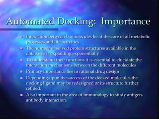
1. The document describes AUTODOCK, an automated docking software used to predict optimal protein-ligand interactions. It summarizes key search algorithms like simulated annealing and genetic algorithms.
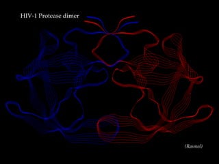
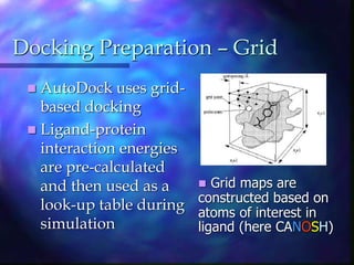
2. As an example application, the document uses AUTODOCK to dock the ligand AHA006 to the HIV-1 protease protein. It describes the preparation steps including assigning charges and defining rotatable bonds.
3. The docking is run using simulated annealing, generating 100 different clusters ranging widely in energy. The lowest energy conformation is not close to the original position, but a higher energy conformation is closest to the original.